

On the intermittent nature of forest fire spread – Part 2†
Domingos Xavier Filomeno Carlos Viegas A * , Jorge Rafael Nogueira Raposo A , Carlos Fernando Morgado Ribeiro A , Luís Reis A , Abdelrahman Abouali A , Luís Mário Ribeiro A and Carlos Xavier Pais Viegas A
A Department of Mechanical Engineering, University of Coimbra, ADAI, Rua Luís Reis Santos, Pólo II, 3030‐788 Coimbra, Portugal.
International Journal of Wildland Fire 31(10) 967-981 https://doi.org/10.1071/WF21098
Submitted: 13 August 2021 Accepted: 1 August 2022 Published: 28 September 2022
© 2022 The Author(s) (or their employer(s)). Published by CSIRO Publishing on behalf of IAWF. This is an open access article distributed under the Creative Commons Attribution-NonCommercial-NoDerivatives 4.0 International License (CC BY-NC-ND)
Abstract
Based on analysis of the interaction between a spreading fire and its surrounding environment, in nominally constant and uniform boundary conditions, it is observed that the evolution of the fire front is characterised by fluctuations of its properties, including (in particular) its rate of spread (ROS). Using a database with a wide range of fires with different time–space scales, it is shown that the amplitude of the fluctuation in ROS is proportional to the average value of the ROS and that the frequency of oscillation varies with the type of fire, and for a given fuel, increases with the average ROS. In fast-spreading fires, the large amplitude of ROS increase and sudden decrease promote the intermittent behaviour of the fire. In general, the amplitude and period required for the ROS increase are larger than for its decrease. However, the acceleration and deceleration phases in junction fires do not follow this rule, suggesting the existence of different convective processes of interaction between the flow and fire. This oscillation explains the variability in many fires at all scales and challenges the current interpretation based on the three factors affecting fire spread and the classification of wind or topography-driven fires.
Keywords: dynamic fire behaviour, fire acceleration, fire growth, fire modelling, fire oscillations, forest fire behaviour, intermittent fire behaviour, oscillatory fire behaviour.
Introduction
Intermittent fire behaviour
Forest fire spread is often analysed as a static process, dependent on a defined set of factors – wind velocity, slope and fuel – which according to some formulations should be sufficient to determine a well-defined value of the rate of spread (ROS) of a fire front (Rothermel 1972, 1983). This concept is a result of the low attention given in the past to the role of convection induced by the presence of fire and its interaction with the surrounding flow (Viegas 2002, 2004a; Finney et al. 2015).
It is interesting to already find in the classical work of Byram (1959), Bruce (1961) a perception of the variability of fire behaviour. Supported by an excellent scientific background and great intuition, and based on observations of many real situations, Byram states that ‘a high intensity fire has a tendency to pulsate or burn in surges, which can produce a rather wide fluctuation in flame length’, and later ‘the fire that remains small or at low intensity is entirely controlled by its environment. It increases in its state of energy production with time, when fuels and burning conditions combine to produce a very high rate of energy release; the fire interacts with its environment and may modify it drastically’. Quoting experienced firefighters, he says that ‘it begins to write its own ticket’, and few lines below, ‘a going fire tends to take on a personality of its own and its dynamics easily equate with the behaviour of a living thing in the mind of a firefighter’. Commenting on the role of wind and topography, Byram says the following: ‘the rate of buildup of fire spread in heavy fuel, in level country, and under the influence of a brisk wind is slowed down when the fire’s intensity becomes high enough to produce a strong indraft opposite the direction of fire spread’. This statement is entirely in line with the conceptual model of intermittent fire behaviour that the authors propose in the first part of the present paper (cf. Viegas et al. 2021). Then, Byram says that ‘this self-regulating process does not occur when a fire builds up intensity when spreading upslope’, which is not correct according to the experience of the authors in the analysis of fires in canyons (cf. Viegas et al. 2021). When dealing with the concept of ‘blow-up’, Byram speaks about a cycle of reinforcement to describe the transition of a low-energy to a high-energy state in fire intensity, which according to his words ‘is seldom a gradual process’, meaning that it goes up in surges that are triggered by factors like an increase of wind speed, local crowning or significant spotting. It is interesting to note that these are all external factors and not necessarily attributable to the fire itself and to its dynamics.
Based on the energy conservation laws, Berlad and Yang (1959) questioned the conditions for existence of a steady state in flame propagation. In Viegas (2004a), it was shown that we could assume steady-state propagation only for fires spreading under no slope and no wind conditions. In the general case, in which neither condition is respected, the ROS depends explicitly on time. For example, in Viegas (2002), it was shown that convection induced by a linear fire front spreading obliquely on a slope modifies its local ROS, producing a rotation of the fire line. Research on the dynamic behaviour of fires was extended to fires in canyons in Viegas and Pita (2004). In Viegas (2004b, 2006), it was shown that fire-induced convection in slopes or canyons produces a feedback on combustion, increasing its ROS. According to the proposed mathematical model, the ROS increases over time after a short period, reaching very high values tending to infinity, although it was felt that this was not possible in real conditions. In the model, an important role is played by the residence time of combustion in the fuel bed, which was used to characterise the dynamic response of the fuel to changes in the ambient conditions (namely wind or slope changes) induced either by external conditions or by the fire itself. In Viegas (2004b), the concept of the ‘square of fire factors’ was introduced, proposing ‘time’ as an explicit factor defining fire spread properties, to account for the dynamic character of combustion.
In the analysis of the junction of two linear fires (Viegas et al. 2012; Raposo et al. 2018), a non-monotonic evolution of the ROS of the head fire was found, with a very rapid increase of the ROS followed by a decrease. In Raposo et al. (2018), this fact was interpreted as an effect of a contrary flow induced by the very rapidly advancing fire, in agreement with Byram’s (1959) statement and showing that this flow could limit the growth of the fire and provide a solution to the problem of an infinite ROS predicted by the mathematical model.
Albini (1982) studied the variability of wind-aided fires, stating that the ROS of fires in natural fuels are very sensitive to wind speed. However, in many cases, the spread rate can also vary substantially with time, even though the fuel and meteorological conditions remain essentially constant. Based on the spectral density of wind fluctuations at frequencies below 0.1 Hz, Albini predicted that the response of the fire would be oscillatory, with a spectral response that depended on the type of fuel and also on the average value of the wind velocity. According to this model, there is a dominant amplitude of oscillation of the ROS for a frequency between 0.01 and 0.02 Hz, but apparently the average value of the ROS is not changed. Although this study grasped some of the features of oscillatory fire behaviour, it did not explain the large amplitude variations of the ROS that are considered in the present paper.
Silvani et al. (2012) analysed the effect of slope on fire spread in laboratory experiments using video images and thermal measurements. From the spectral analysis of gas temperature and total heat flux density, they found an increase in frequency of fluctuations when the slope was increased from 0° to 30°.
In a previous study (Viegas et al. 2021), the authors proposed a conceptual model for the development of a fire under nominally constant and uniform boundary conditions, showing how the interaction of natural convection produced by the fire and the surrounding environment induces a cyclic modification of the flame geometry, causing the fire to spread in an oscillatory manner. This concept was supported by experimental data showing how the overall shape of the flame was modified for a point ignition fire in a slope or a canyon and its effect on the flow across the flame region and its ROS variation with time.
Scope of the paper
The purpose of the present paper is to highlight the fact that the process of fire spread, even in nominally constant and uniform boundary conditions, is composed of oscillations deriving from the interaction between the combustion processes and the ambient flow surrounding the fire. This is reflected, for example, in the temporal evolution of the ROS, which has oscillations of varying amplitude and frequency. As a result of some considerable amplitude oscillations, the fire spreads in an intermittent form, with marked increases of the ROS followed by sudden decreases, even under permanent boundary conditions. The proposed concept is supported by experimental evidence from fires covering a wide range of space and time conditions, corresponding to virtually all practical situations that can be expected in forest fire spread.
Methodology
A note on fire dynamics
We consider a fire that is spreading with a flaming fire front on a fuel bed at or near the surface of the ground. The balance of energy exchanged between the combustion regions inside and above the fuel, the environment and the unburned fuel ahead of the fire front, considering radiation, convection and conduction, provides as an outcome the rate of advance of the fire front in the fuel bed (cf. Albini 1981, 1982; Weber 1989). This ROS of the fire front is a critical parameter in the analysis of fire behaviour, as many other fire spread properties, like fire line intensity, fuel consumption, smoke emission, the possibility of extinction, perimeter or burned area growth, are related to it.
For each point P on the surface on which the fire is spreading, we can assign the following parameters P (x, y, t) in which x and y are the coordinates that define the position of the point and t is the time of arrival of the fire at the point.
Although we can define the ROS at each point of the fire line, the head ROS of the most advanced or fast-spreading section of the fire is of particular relevance. Knowing this ROS and the capacity to estimate its evolution in time and space are of great practical importance, as it contains an indication of where the fire is spreading, how fast it is growing, and what can be done to avoid it or suppress it.
The oscillatory processes considered in this paper occur over the entire fire area, as they have a three-dimensional character, as remarked by Finney et al. (2015). In the present paper, we are concerned with the analysis of fire spread and its oscillations along its main direction of spread, characterised by a curvilinear or quasi-linear coordinate x, having in mind that the trajectory of the head fire may not be a straight line. Using an analogy, this is equivalent to considering the three-dimensional undulation that can be observed on the surface of the sea near the shore. In the analysis, we can consider a direction perpendicular to the coast and analyse the properties of the waves along that line. In this paper, we do the same regarding the spread of the fire.
Along this line that contains the head of the fire, each point is characterised by P(x, t). Alternatively, we can use the ROS R, defined by:
Knowing R, we can determine x by integrating Eqn 1 for the time from the fire origin until t, and therefore we can characterise each point either by P(R, t) or by P (R, x). This means that we can use x, R or t as independent variables as required in the analysis of fire spread.
At each point of this trajectory, the fire will have a particular value R(x). As each point is reached at a definite time t, we will use time to describe the evolution of ROS during fire spread R(t).
Fire factors
It is well known that the properties of fire spread depend on the following set of factors, which is designated the ‘square of fire factors’ (Viegas 2004b): (i) topography, (ii) fuel, (iii) meteorology, and (iv) time.
There is ample evidence in the literature on the role and relevance of these factors, separately or acting together (Chandler et al. 1983). We briefly mention some key parameters that characterise each of these factors to set the stage for the subsequent analysis of the oscillatory evolution of the fire.
Topography
Among the various parameters required to define terrain topology around the place where the fire may be spreading, we retain two: (i) the terrain inclination angle α (°), or simply the slope; and (ii) the terrain curvature, which characterises its convex or concave shape. In this context, concave-shaped terrain, like gullies or canyons, is of particularly importance, as they are prone to very fast eruptive fires (Viegas 2004a, 2004b).
Fuels
A surface fuel bed is characterised by a wide set of parameters (Rothermel 1972, 1983), namely the fuel load Mc (kg m−2), fuel bed height h (m), compactness β (−), particle minimum dimension d (cm) or its equivalent surface-to-volume ratio σ (cm−1), and the moisture content mf (%) of the particles. In the case of simple fuel beds composed of uniform particles, which many laboratory experiments use, we can estimate these parameters easily. However, in real fuel beds where we have a mixture of particles of different sizes, shapes and properties, it is necessary to use averaging methods like those proposed by Rothermel (1983), Viegas et al. (2013) or Weise et al. (2022) to estimate representative values of those parameters. Therefore, for the present study, we retain three parameters: mf, Mc and σ or, as an alternative, the minimum dimension d (m) of the fuel particles, knowing that in general σ ≈ 1/d.
Meteorology
Among the various meteorological parameters relevant to fire spread, we consider those associated with modification of the fuel moisture content, the spread of the fire, mainly wind velocity and direction, and the stability of the atmosphere. For simplification, we assume that the fuel moisture content – which depends primarily on solar radiation, precipitation, air temperature, relative humidity and wind – is included in the fuel bed properties, and retain wind velocity U as the single meteorological parameter affecting the ROS.
Time
Current texts on fire spread do not consider chronological time explicitly as a parameter or factor in fire behaviour analysis, as most studies consider average values of the fire spread properties. Time was proposed by Viegas (2004b) as an explicit factor in recognition of the dynamic character of fire behaviour, meaning that in cases in which all the parameters mentioned above remain constant in space or permanent in time, the properties of fire spread may change owing to the interaction between the fire and its surroundings. Examples of this are the spread of a point ignition fire in a slope or a canyon (cf. Viegas 2004a).
In this paper, we consider the variation of ROS over time in fires that spread ideally on a uniform fuel bed, on a terrain with uniform configuration (constant slope or curvature) and in a constant and permanent ambient wind flow.
It is easy to recognise that such conditions only exist in the case of very controlled laboratory experiments. In field experiments or real fires, even if some factor (like wind or slope) may be dominant, some parameters, like fuel cover, may change, introducing uncertainty in the analysis.
Oscillatory fire behaviour
There is evidence in the literature (Wade and Ward 1973; Simard et al. 1983; Rothermel and Mutch 2003) and in the analysis of fire spread at various scales that even in nominally permanent and uniform boundary conditions, ROS does not remain constant, but evolves with oscillations that can reach quite high values, like in the case of eruptive fires, and decrease suddenly in an intermittent form. We can observe these processes over a wide range of space and time as illustrated by the three examples shown in Fig. 1. In Fig. 1a, we see the evolution of R as a function of time or distance travelled by the head fire in a laboratory experiment of a point ignition fire in a canyon (Test DE301). In Fig. 1b, we have the results from a field experiment of a linear fire spreading upslope (Test 807), and in Fig. 1c, we have the estimated values of R in the case of the Sundance fire (Anderson 1968), also as a function of time or distance.

|
We used the same units in all graphs to highlight the variation of the parameters involved and the prevalence of the oscillatory behaviour of fire spread in all cases.
Amplitude and period of oscillations
To characterise the properties of the oscillatory behaviour of fire spread, we estimate the amplitude and period or frequency of these oscillations.
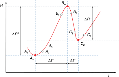
As the previous cases illustrated, we can use either time or distance to describe the evolution of the fire spread in a given direction. From now on, we consider the domain (R, t) as represented in Fig. 2, in which each point P(R, t) is a vector characterised by a pair of values, of the ROS R and time t. The line defined by points A1, A2, …, C2, represents the idealised evolution of R during a period in which a full cycle of oscillation between Ao and Co can be seen. Points Ao and Co are two local minima and Bo is a local maximum.
|
Our observations indicate that the cycle is not symmetrical, so we consider two separate half-periods, one of R increase, between Ao and Bo, and another of R decrease between Bo and Co.
We introduce the following definitions:
Amplitude of ROS increase: ΔR+ given by the difference of ROS at Bo and at Ao
Amplitude of ROS decrease: ΔR− given by the difference of ROS at Bo and at Co
Half-period of ROS increase: Δt+ given by the difference of time at Bo and at Ao
Half-period of ROS decrease: Δt− given by the difference of time at Co and at Bo
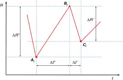
Given the limitations of data acquisition processes in real fires, in field experimental fires and even in laboratory experiments, in many situations, we do not have a full trace for R(t) but just a set of discrete points like those shown in Fig. 3. In the absence of more detailed data, we have to assimilate points Ai, Bi and Ci with Ao, Bo and Co.
|
Having in mind that any of these points may not coincide with the actual local extreme values, this assumption will be a source of error in the evaluation of both Δt and ΔR. For example, Ai can be either A1, A2, or A3 (cf. Fig. 2) instead of Ao and the same may happen with the other two points. Depending on the temporal resolution of the ROS data, the error in the estimate of both Δt or ΔR can be as high as 100%, meaning that the actual value of those parameters estimated from non-complete data can be either half or double the estimated value.
As the present analysis is based on experimental data collected at different scales and from different sources, it can be argued that the observed fluctuations can be related to measurement errors, as described by Fujioka (2002). We checked the source of error in estimating ROS values and found that the error of measurement can be of the same order of ΔR only for some of the laboratory experiments with R < 0.1 cm s−1, but in all other cases, including the real fires, the amplitude of oscillations is much larger than the estimated measurement error.
Analysis of amplitude of oscillations
Considering two points P1 and P2 in the space (R, t) so that P1 ≡ Ao and P2 ≡ Bo, and R1 < R2 we can define:

And:
If we consider now points P2 ≡ Bo and P3 ≡ Co, we define the amplitude ΔR−:

We use this definition in order to have essentially positive values of the amplitude of oscillation.
We defined two values for the amplitude of oscillation, one for the increasing phase of the cycle and another for the decreasing phase, assuming that they are different. This is generally confirmed by our present data, which indicates that ΔR+ > ΔR−. In this study, we also refer to the amplitude of oscillation ΔR, regardless of it being one or the other.
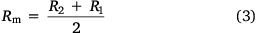
In estimating the arithmetic mean value Rm to characterise the oscillation represented by the pair of values R1 and R2, we decided to use the arithmetic mean instead of the geometric or harmonic mean (cf. Fujioka and Fujioka 1985; Weise and Biging 1994), because we do not intend to specify the ‘average ROS’ of the fire between the two points P1 and P2, as this would require information that we do not have in many cases. Besides this, contrary to the harmonic mean, which gives a higher weight to the lowest value, the arithmetic mean is at equal distance from both values.
Analysis of frequency of oscillations
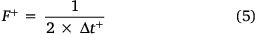
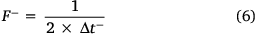
To each half period Δt+ and Δt− defined above, we can assign a frequency of oscillation F+ and F−, given respectively by:
The physical unit of these frequencies is hertz (s–1). The present data indicate that F+ < F−, meaning that in general, the period of time required for fire growth is larger than for ROS decrease. We also define a single value of the frequency of oscillation F given either by F+ or F−.
We could have defined the frequency with a single equation, without distinguishing between F+ and F−, but as in the case of the amplitude for the accelerating and decelerating half periods, we decided to retain these definitions to highlight the different behaviour of the fire observed in each half cycle.
Study cases
There are many situations in which the oscillatory or intermittent behaviour of fire, with an initial acceleration followed by a quick deceleration, have been observed and documented. To analyse the oscillatory nature of fire spread, we selected a series of cases with data on the variations of ROS with time from which we can estimate the amplitude and period of R oscillations. These cases cover a wide range of situations found in fire science studies. They include results produced by the present authors in laboratory and field-scale experiments, and also real fires reported in the literature.
Here, we give a brief description of the study cases used in this investigation, and more details are provided in Supplementary Appendices S1–3.
Laboratory-scale experiments
The experiments reported in this paper were performed by the authors or by other members of their research team at the Fire Research Laboratory of the University of Coimbra, using several test rigs but mainly Combustion Table DE4 (cf. Viegas et al. 2012, 2021; Raposo et al. 2018). All tests reported here were performed with a fuel bed composed of dead needles of Pinus pinaster, with a load Mc of 0.6 kg m–2 (dry basis).
We used the following three sets of tests:
Point ignition fire on a slope (SP) with an inclination angle α equal to 20°, 30° and 40°;
Point ignition fire in a canyon (DE) with an inclination angle α equal to 20°, 30° and 40°;
Junction fire on a slope (JF) with an inclination angle α equal to 20°, 30° and 40°.
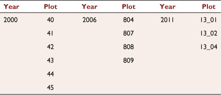
The reference codes of the tests used are given in Table 1. More details can be found in Supplementary Appendix S1.

|
Field-scale experiments
The reference codes for the plots of the file experiments are given in Table 2. More details can be found in Supplementary Appendix S2.
|
Real fires
From the large amount of data available in the literature reporting the spread of large fires, we selected eight cases in which the oscillatory behaviour of the head fire at different scales was evident, see Table 3. These cases were chosen because during their spread, a major factor – usually wind – remained practically constant in speed and direction, rendering justification of the variations in ROS by changes in the ambient factors unconvincing. In the Supplementary Appendix S3, a brief description of each fire and the relevant references are given.

|
Results and discussion
Amplitude of oscillations
From analysis of the cases mentioned above, we estimated the values of ΔR and Rm shown in Fig. 4.

|
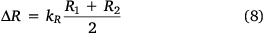
As can be seen in that figure, the data points cover a range of more than three orders of magnitude, from 0.22 to 514 cm s–1 in Rm and a similar range for ΔR as well. Given the apparent linear relationship between the amplitude ΔR of the oscillations and the mean value Rm of the ROS, we can express it as:

In Fig. 4, a straight line fitting of the entire data set is shown, and the corresponding value of kR is equal to 1.276. The two lines that are shown in the figure correspond to values of kR of 2.0 for the upper line and 0.2 for the lower line. We chose a line passing by the origin of the coordinate system assuming that for Rm = 0, there should be no oscillations and therefore it should also be ΔR = 0.
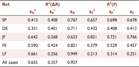
We analysed the fitting of Eqn 7 to sets of partial data for each of the five cases studied. For each case, we considered ΔR+, ΔR− and ΔR, and obtained the respective values of kR that are given in Table 4. The corresponding values of R2 are given in Table 5.

|
|
The relevance of the data in Fig. 4 is to show the existence of a relationship between Rm and ΔR, which is a monotonic increasing function in the entire range of data. Having used the arithmetic mean, this function is well represented by a linear function. We tested other methods to calculate the mean value of Rm; using for example harmonic means, a monotonic increase of ΔR with Rm is found as well, but with a large amount of scatter.
The ratio kR+/kR− is usually larger than one, indicating that on average the amplitude of fire growth oscillations is larger than those of fire spread decrease, as was assumed above.
Two-way ANOVA without replication for values presented in Table 4 indicated that the kR values were significantly different (P value < 0.05) for positive, negative and all data values for all different scales used. However, two-way ANOVA without replication showed that for the kF values for each type of scale analysed, the results were significantly different (P value < 0.05), but for a different analysis of kF values (positive, negative and all data), they were not significantly different (P value > 0.05).
To analyse the meaning of coefficient kR on the variation of ROS during an oscillation, we consider that R2 > R1; therefore:
It is easy to conclude that:
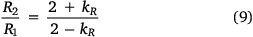
The evolution of the ratio between R2/R1 as a function of kR according to Eqn 9 is shown in Fig. 5.

|
As shown in Fig. 4 and in Table 4, the value of kR estimated for partial sets of data indicates three typical values: between 0.4 and 0.8 for laboratory-scale experiments, 0.9 for field experiments, and 1.3 for large fires. This means that the ratio R2/R1 between the local maximum and minimum values of the ROS during a period of oscillation increases with the scale of the fire, and may reach values of 4 or 5 in large fires.
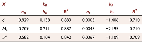
Our data indicate that kR varies with the type of fire considered. Despite the limited amount of data available, we attempt to establish correlations of kR with three proposed parameters: (i) the typical dimension d (cm) of the largest fuel particles consumed by the fire during its propagation; (ii) the typical fuel load Mc (kg m–2) consumed by the fire, and (iii) the typical overall dimension  (m) of the fire, assuming that it is spreading as a coherent convective cell. In very large fires, we may have various fire cells or sections of the fire along the perimeter of the fire, possibly with different heads. In such cases, each cell must be treated separately.
In this paper, we do not intend to provide very accurate data on the characteristics of each fire, namely to provide an average value of each of the proposed parameters following, for example, Weise et al. (2022), but rather to give typical values representative of the order of magnitude of each parameter in the range of studied cases. In the laboratory experiments, d and Mc can be defined with great precision, respectively, as 0.06 cm, 0.6 kg m–2, as they were kept constant in the whole set of experiments used in this study. The dimension  of the fire can be set to 3 m, which was the typical size of the fuel beds used in the experiments. For the field experiments, we considered that the largest particles consumed by the fire had a thickness up to 2 cm, and that the fuel load was on average 4 kg m–2. For the fire scale, we took a value of 40 m, which was a typical width of the experimental plots (cf. Supplementary Table S3 in Supplementary Appendix S2). For the natural fires, it is more difficult to estimate average values of these parameters, and we considered, somewhat arbitrarily, the following indicative values: d = 10 cm, Mc = 20 kg m–2 and
  = 4000 m.
In Fig. 6, we plot kR as a function of the three characteristic parameters considered: d, Mc and  . In each case, we applied a power-law fitting of the type:

In Eqn 10, parameter X is either d, Mc or  , and the corresponding coefficients of the equation are given in Table 6. In spite of the uncertainty of this analysis, we can see that kR has a relatively small variation with each of them, indicated by the exponent of the order of 0.1 to 0.2 found in the power law fitting. We do not provide any physical interpretation for this power law function, other than observing that the parameters aR and bR are always of the same order of magnitude and that the modulus of bR is quite small.

|
 .
.
|
Frequency of Oscillations
From analysis of the cases described above, we estimated values of the frequency of the oscillations of the ROS, illustrated in Fig. 7. As shown, the frequency of oscillations varies in a range of five orders of magnitude, from 6 ×10⁻⁶ Hz (corresponding to a period of ~46 h) to 0.1 Hz (corresponding to a period of 10 s).

|
In spite of the scatter of the data, we can identify three main groups of results, corresponding to the three scales of the experimental data: laboratory, field and large fires.
For a given type of fuel, we can express an approximately linear relationship between F and R, for given sets of data, as:

As in the previous case where we tested a correlation between ΔR and Rm, in this case, we fit a linear function with zero origin to the distribution of F and Rm for certain ranges of values. According to Eqn 11, coefficient kF has units of (cm−1), the same as σ. Following the methodology described above, we estimated the values of kF+, kF− and kF for each set of data, and the results are given in Table 4. In contrast to kR, the coefficient kF shows large variation – four orders of magnitude – from one fuel to the other, so there is no point in defining an overall average value of kF for the entire data set.
As shown in Table 4, the ratio between kF+/kF− is essentially lower than one, meaning that on average Δt+ > Δt−, as indicated above in the definition of the half-periods of oscillation. This means that the process of fire acceleration takes on average more time than the decreasing phase, indicating that the mechanisms that govern each half cycle are different. We will analyse these differences in more detail in future work. Tests of junction fires show a different trend, with kF+/kF− > 1, meaning that in this type of fire, the convective processes have a different role during the acceleration and the deceleration phases. These processes have already been studied in Viegas et al. (2012), Raposo (2016) and Raposo et al. (2018), but require further investigation.
Following the analysis performed above, we plotted in Fig. 8 the variation of kF with each parameter describing the fire spread conditions, namely d, Mc and  . The coefficients aF and bF of a power-law fitting given by Eqn 12 are given in Table 6.

Given the very crude approximations made in estimating these parameters, we cannot extract many conclusions or physical interpretations from those relationships. However, it is interesting to note that coefficient aF varies by two orders of magnitude and exponent bF varies between 1.1 and 2.1, indicating a much stronger dependence of the frequency of oscillations on the selected parameters. We require more data to extract more definitive conclusions on the role and relationship of the identified parameters.

|
 .
.Residence time
The period of the natural oscillations of the fire is related physically to the duration tr of the combustion process in the fuel bed, or residence time of the flame. According to Nelson (2003), we assume that the residence time of the flame (or flameout time of a particle) is the same as the reaction time (travel time of the fire front for a distance equal to the flame depth). For a given fuel bed, we should have:
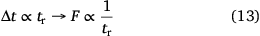
The residence time tr of the flame can be measured experimentally or estimated from the fuel bed’s properties using models. Vaz et al. (2004) studied various empirical models to estimate the residence time of fuel beds based on their physical properties. They report one model proposed by Fons 1946, for relatively thick particles (d > 4 mm), that proposes tr ∝ d1.5. Referring to Eqn 13, we can conclude that this law is very close to the present finding that kF ∝ d1.4. In contrast, another model by Anderson (1982) proposes a linear relationship between tr and d.
In Vaz et al. (2004), the influence of the ROS of the fire on tr is not addressed directly, although some results on the effect of moisture content mf may include this effect. In a series of experiments with crib fires, it was observed that tr increased with mf. As the ROS decreases with mf, it can be inferred that tr decreases with R, as we found in experiments carried out on a slope with pine needles as a fuel bed. We measured the air temperature 14 cm above the ground inside the flames with a K-type thermocouple and considered that the duration of the temperature trace above 350°C corresponded to the residence time tr of the flame. The values of tr obtained are plotted in Fig. 9 as a function of the local value of R. There is great scatter of the data, but a linear fit given by Eqn 14 indicates a negative slope, confirming the decreasing tendency of tr (s) with R (cm s−1).

Using Eqn 14 to calculate 1/tr in the interval 0.3 < R < 3 cm s–1, the values obtained can be fitted by (centimetre–gram–second (CGS) system of units):
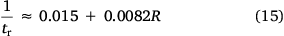
If we assume that tr ≈ Δt according to Eqns 5, 9, for the laboratory tests with pine needles, we should have kF ≈ 0.0041, which is smaller than, but of the same order as the values estimated above (0.006 < kF < 0.012). A line corresponding to Eqn 15 in the range of values of Rm was plotted in Fig. 4.

|
In Viegas (2004a), the residence time tr (in that paper and some subsequent works, it was designated to) was considered as a relevant parameter of the dynamics of fire behaviour in a given fuel bed. In the differential equation derivation of the eruptive fire model, it was assumed that this value was constant for a given fuel bed. The present results indicate that this assumption has to be revised.
In Viegas (2006), typical values of the residence time for various types of fuels were proposed, with an indication of the minimum, maximum and average estimated values of tr for each. These values are presented in Table 7 in which litter, shrub and slash correspond respectively to pine litter, field experiments and heavy surface fuels like those found in high-intensity fires. Calculating the corresponding frequency of oscillation using Eqn 5, we obtain the values given in the table. It can be seen that these values follow the trend found in the present study for the range of variation of the oscillations frequency.

|
Discussion
Interpretation of the evolution of a head fire as a sequence of oscillations, with a well-defined amplitude and half-period duration, is supported by experimental data from different sources. The proposed study cases used to illustrate the model cover a wide range of time and space scales and types of vegetation cover. The common aspect in all of them is the existence of nominally constant or uniform boundary conditions for fire spread (wind, fuel and topography). In the laboratory experiments, wind was absent, but terrain configuration was constant, whereas in almost all large fire cases, wind was blowing with a constant direction and with a fairly high and practically constant velocity.
In all cases, we found a regular distribution of the amplitude of oscillation ΔR, proportional to the average value of Rm. The constant of proportionality kR varies between 0.3 and 1.3 for the entire range of R, covering more than three orders of magnitude. Smaller-scale fires seem to have lower values of kR whereas large fires tend to have higher values. Consequently, the ratio between the maximum and minimum value of R in a period of oscillation can be larger than 3 in very large fires.
The amplitude of oscillation and the half-period in the fire increase phase are usually larger than that of the decreasing phase. However, there is a remarkable exception for junction fires, in which the opposite is observed for the period of oscillation. This fact is undoubtedly due to the very intense and unusual convective processes in this type of fire, but this is a problem that requires further investigation.
The frequency F of the natural oscillations of the ROS covers five orders of magnitude and seems to depend on at least two factors: the type of fire and the ROS. Our results indicate that for a given type of fire or fuel bed, the frequency of oscillation increases linearly with R. We tested three parameters to characterise the type of fire: the size of the consumed particles, the fuel load and the size of the fire. These indicate the possible dependence of kF with the type of data available.
The residence time of flaming combustion must be associated with the oscillation period. Some results of independent measurement of residence time for a pine needle fuel bed yielded the same tendency found for kF in laboratory experiments.
We give a word of caution to fire spread models that do not consider the oscillations described in this paper. Most models assume that fire is spreading under steady conditions and provide only an average ROS value. If the prediction is accurate, the model will estimate the time of arrival of a fire at a given point with great precision, but it will not consider that in the process, it may have ROS values 3–5 times the average value, and this is not acceptable, especially in the context of fire safety (cf. Case 6 of the Butte fire). This fact shows the intrinsic difficulty in applying current fire behaviour models based on experimental data obtained at laboratory or field scale to predict the behaviour of large fires, as the amplitude of oscillations is much smaller. This is possibly why Rothermel (1991) reported that the ROS of some large fires was on average 3.34 times higher than the values predicted by his model.
Byram (1959), Bruce (1961) introduced the concepts of power of wind and power of fire to describe the interaction between a large fire and the atmosphere and proposed the designations of wind-dominated or convection or plume-dominated fires. Rothermel (1991) used these concepts when analysing the behaviour of very large fires and suggested that the two most prominent fire behaviour patterns in these fires were ‘wind-driven fires’ and ‘plume-dominated fires’, inferring that these were two completely different and separate types of fires. Nelson (1993, 2003) recovered Byram’s original work and developed it with a mathematical formulation to check its applicability to real situations. Based on our observations of the oscillatory behaviour of fires and the relatively large amplitude and long periods of oscillation of very large fires, we question the proposed designations of ‘wind-dominated’ or ‘plume- or topography-dominated fires’ that are widely used in fire science and practice. In our opinion, a spreading fire may have a phase in which it spreads very fast and with a very inclined convection column – in the ROS increase phase – that is indeed a wind-dominated phase of the fire. What we designate as wind is the composition of ambient wind plus fire-induced wind, which can dominate. The designation of ‘conflagration’ is also applicable to this phase of a fire, especially if the ambient wind velocity is quite high. When the convection column becomes more vertical – in the decreasing ROS phase – people say that the fire is ‘convection-dominated’ or even that it is a ‘topographic fire’, implying that wind is not playing a role in fire behaviour in this phase, which is not correct. Wind and topography, like convection, are usually present during the entire fire development. This phase of the fire can also be designated as ‘mass fire’ as a large mass of fuel is burning without a large ROS value.
The convection generated by a fire and the way it modifies the surrounding wind flow promote the changes in fire behaviour: one phase of the fire follows the other. In the general case, there are no pure wind or convection-dominated fires. There are periods of time in which fires spread like a conflagration, while in others, they behave like a mass fire.
The existence of relatively long periods of oscillation – tens of minutes – in very large fires can be of great practical importance as the phase with lower ROS values can be used to attack the fires more safely or to promote local evacuation or deployment of personnel. Consequently, the ability to predict the exact occurrence of these phases is of great relevance, and therefore an understanding of the oscillatory motion reported in this paper needs to be improved.
Conclusion
In this paper, based on data from virtually all scales of fires of practical interest, we showed that an oscillatory motion characterises the spread of a fire. This natural oscillation results from the combustion processes and their interaction with the surrounding atmosphere. This oscillation is analogous to the breathing process of a living animal and it is an intrinsic property of a given spreading fire, with a well-defined frequency and amplitude of oscillation.
As a result, the ROS of any section of the fire, for example (in this case, in particular) of its head or most advanced section, varies in time and space, with oscillations composed of a half-period of R increase followed by a half-period of R decrease. The amplitude of these oscillations is proportional to the average value of R and the constant of proportionality is slightly dependent on the type of fire, namely on its size. Larger fires tend to have relatively higher amplitudes of oscillation.
The frequency of oscillation of the variation in R covers more than five orders of magnitude in the range of fires that we studied. Our preliminary data seem to indicate that the frequency of oscillation depends on the type of fire and its ROS. For a given fuel bed and type of fire (characterised by its scale or mass load), the oscillation frequency increases linearly with R.
The cases of large fires analysed from the literature illustrate well the reality of the intermittent behaviour of fires under permanent and uniform conditions. The difficulty in explaining the rapid changes in fire behaviour – in particular the rapid decrease of ROS – due to the framework and mindset of the ‘triangle of fire factors’ was very evident in the review performed.
We intend to explore more experimental data to complement the proposed analysis and model formulation in future work. In particular, we intend to use the better capacity now available to record and analyse the spread of a fire front with greater time resolution and the flow changes near the fire to better characterise and estimate the amplitude and frequency of oscillations.
Data availability
Data are available only under request to the corresponding author: Domingos Xavier Viegas, xavier.viegas@dem.uc.pt.
Conflicts of interest
The authors declare that they have no conflicts of interest.
Declaration of funding
The work reported in this article was carried out in the scope of project Firestorm (PCIF/GFC/0109/2017), McFire (PCIF/MPG/0108/2017), IMfire (PCIF/SSI/0151/2018), Region (Centro 2020, Centro-01-0246-FEDER-000015) and project (Centro 2020, Centro-01-0145-FEDER-000007) supported by the Portuguese National Science Foundation and the European Union’s Horizon 2020 Research and Innovation Programme under grant agreement No. 101003890. We would like to thank the FCT-Foundation for Science and Technology for the Carlos Ribeiro’s PhD grant, with reference no. SFRH/BD/140923/2018.
Author contributions
Conceptualisation: Domingos Xavier Viegas; data curation: Domingos Xavier Viegas, Carlos Ribeiro and Abdelrahman Abouali; formal analysis: Domingos Xavier Viegas, Jorge Raposo and Carlos Ribeiro; methodology: Domingos Xavier Viegas, Jorge Raposo, and Carlos Ribeiro; experimental tests: Jorge Raposo, Carlos Ribeiro, Luís Reis and Abdelrahman Abouali; supervision: Domingos Xavier Viegas; Writing, original draft: Domingos Xavier Viegas; writing, review and editing: Domingos Xavier Viegas, Jorge Raposo, Carlos Ribeiro, Luis Reis, Abdelrahman Abouali, Luis Ribeiro and Carlos Viegas.
Symbols
Supplementary material
Supplementary material is available online.
Acknowledgements
The support of Daniela Alves, Claudia Pinto and Nuno Luis in the laboratory experiments and in the preparation of some figures of this article is gratefully acknowledged.
References
Albini FA (1981) A model for the wind-blown flame from a line fire. Combustion and Flame 43, 155–174.| A model for the wind-blown flame from a line fire.Crossref | GoogleScholarGoogle Scholar |
Albini FA (1982) Response of free-burning fires to non-steady wind. Combustion Science and Technology 29, 225–241.
| Response of free-burning fires to non-steady wind.Crossref | GoogleScholarGoogle Scholar |
Anderson HE (1968) The sundance fire: an analysis of fire phenomena. USDA Forest Service, Intermountain Forest and Range Experiment Station Research Paper INT-56. (Ogden, UT) Available at https://www.fs.usda.gov/treesearch/pubs/32534
Anderson HE (1982) Aids to determining fuel models for estimating fire behavior. USDA Forest Service, Intermountain Forest and Range Experiment Station General Technical Report INT-122. (Ogden, UT). Available at https://www.fs.usda.gov/treesearch/pubs/6447
Berlad AL, Yang CH (1959) On the existence of steady state flames. Combustion and Flame 3, 447–452.
| On the existence of steady state flames.Crossref | GoogleScholarGoogle Scholar |
Bruce GM (1961) Forest fire control and use. Ecology 42, 609–610.
| Forest fire control and use.Crossref | GoogleScholarGoogle Scholar |
Byram GM (1959) Combustion of forest fuels. In ‘Forest fire: control and use’. (Ed. KP Davis) pp. 90–123. (McGraw-Hill: New York, NY)
Chandler C, Cheney P, Thomas P, Trabaud L, Williams D (1983) ‘Fire in forestry. Vol. 1. Forest fire behavior and effects.’ (John Wiley & Sons, Inc.: New York)
Finney MA, Cohen JD, Forthofer JM, McAllister SS, Gollner MJ, Gorham DJ, Saito K, Akafuah NK, Adam BA, English JD (2015) Role of buoyant flame dynamics in wildfire spread. Proceedings of the National Academy of Sciences 112, 9833–9838.
| Role of buoyant flame dynamics in wildfire spread.Crossref | GoogleScholarGoogle Scholar |
Fons WL (1946) Analysis of fire spread in light forest fuels. Journal of Agricultural Research 72, 93–121.
Fujioka FM (1985) Estimating wildland fire rate of spread in a spatially non-uniform environment. Forest Science 31, 21–29.
Fujioka FM (2002) A new method for the analysis of fire spread modeling errors. International Journal of Wildland Fire 11, 193–203.
| A new method for the analysis of fire spread modeling errors.Crossref | GoogleScholarGoogle Scholar |
Nelson RM (1993) Byram derivation of the energy criterion for forest and wildland fires. International Journal of Wildland Fire 3, 131–138.
| Byram derivation of the energy criterion for forest and wildland fires.Crossref | GoogleScholarGoogle Scholar |
Nelson Jr RM (2003) Power of the fire – A thermodynamic analysis. International Journal of Wildland Fire 12, 51–65.
| Power of the fire – A thermodynamic analysis.Crossref | GoogleScholarGoogle Scholar |
Raposo JR, Viegas DX, Xie X, Almeida M, Figueiredo AR, Porto L, Sharples J (2018) Analysis of the physical processes associated with junction fires at laboratory and field scales. International Journal of Wildland Fire 27, 52–68.
| Analysis of the physical processes associated with junction fires at laboratory and field scales.Crossref | GoogleScholarGoogle Scholar |
Raposo JRN (2016) Extreme fire behaviour associated to merging of two linear fire fronts. PhD Thesis. Coimbra University, Spain. Available at http://hdl.handle.net/10316/31020
Rothermel RC (1972) A mathematical model for predicting fire spread in wildland fuels. USDA Forest Service, Intermountain Forest and Range Experiment Station, Research Paper INT-RP-115. (Ogden, UT)
Rothermel RC (1983) How to Predict the Spread and Intensity of Forest and Range Fires. USDA Forest Service General Technical Report INT-143.
Rothermel RC (1991) Predicting behavior and size of crown fires in the northern Rocky Mountains. USDA Forest Service, Intermountain Research Station, Research Paper 46.
Rothermel RC, Mutch RC (2003) Behaviour of the life-threatening Butte Fire: August 27–29, 1985. Fire Management Today 63, 31–39. Available at https://www.fs.usda.gov/sites/default/files/legacy_files/fire-management-today/63-4.pdf
Silvani X, Morandini F, Dupuy J-L (2012) Effects of slope on fire spread observed through video images and multiple-point thermal measurements. Experimental Thermal and Fluid Science 41, 99–111.
| Effects of slope on fire spread observed through video images and multiple-point thermal measurements.Crossref | GoogleScholarGoogle Scholar |
Simard AJ, Haines DA, Blank RW, Frost JS (1983) The Mack Lake Fire. USDA Forest Service, North Central Forest Experiment Station, General Technical Report NC-83. (St Paul, MN).
Vaz GC, André JCS, Viegas DX (2004) Fire spread model for a linear front in a horizontal solid porous fuel bed in still air. Combustion Science and Technology 176, 135–182.
| Fire spread model for a linear front in a horizontal solid porous fuel bed in still air.Crossref | GoogleScholarGoogle Scholar |
Viegas DX (2002) Fire line rotation as a mechanism for fire spread on a uniform slope. International Journal of Wildland Fire 11, 11–23.
| Fire line rotation as a mechanism for fire spread on a uniform slope.Crossref | GoogleScholarGoogle Scholar |
Viegas DX (2004a) On the existence of a steady state regime for slope and wind-driven fires. International Journal of Wildland Fire 13, 101–117.
| On the existence of a steady state regime for slope and wind-driven fires.Crossref | GoogleScholarGoogle Scholar |
Viegas DX (2004b) A mathematical model for forest fires blowup. Combustion Science and Technology 177, 27–51.
| A mathematical model for forest fires blowup.Crossref | GoogleScholarGoogle Scholar |
Viegas DX (2006) Parametric study of an eruptive fire behaviour model. International Journal of Wildland Fire 15, 169–177.
| Parametric study of an eruptive fire behaviour model.Crossref | GoogleScholarGoogle Scholar |
Viegas DX, Pita LP (2004) Fire spread in canyons. International Journal of Wildland Fire 13, 253–274.
| Fire spread in canyons.Crossref | GoogleScholarGoogle Scholar |
Viegas DX, Raposo JR, Davim DA, Rossa CG (2012) Study of the jump fire produced by the interaction of two oblique fire fronts. Part 1. Analytical model and validation with no-slope laboratory experiments. International Journal of Wildland Fire 21, 843
| Study of the jump fire produced by the interaction of two oblique fire fronts. Part 1. Analytical model and validation with no-slope laboratory experiments.Crossref | GoogleScholarGoogle Scholar |
Viegas DX, Soares J, Almeida M (2013) Combustibility of a mixture of live and dead fuel components. International Journal of Wildland Fire 22, 992–1002.
| Combustibility of a mixture of live and dead fuel components.Crossref | GoogleScholarGoogle Scholar |
Viegas DXFC, Raposo JRN, Ribeiro CFM, Reis LCD, Abouali A, Viegas CXP (2021) On the non-monotonic behaviour of fire spread. International Journal of Wildland Fire 30, 702–719.
| On the non-monotonic behaviour of fire spread.Crossref | GoogleScholarGoogle Scholar |
Wade DD, Ward DE (1973) An analysis of the Airforce Bomb Range Fire. USDA Forest Service, Southeastern Forest Experiment Station, Research Paper SE-RP-105. (Asheville, NC)
Weber RO (1989) Analytical models for fire spread due to radiation. Combustion and Flame 78, 398–408.
| Analytical models for fire spread due to radiation.Crossref | GoogleScholarGoogle Scholar |
Weise D, Biging G (1994) Effects of wind velocity and slope on fire behavior. Fire Safety Science 4, 1041–1051.
| Effects of wind velocity and slope on fire behavior.Crossref | GoogleScholarGoogle Scholar |
Weise DR, Fletcher TH, Safdari MS, Amini E, Palarea-Albaladejo J (2022) Application of compositional data analysis to determine the effects of heating mode, moisture status and plant species on pyrolysates. International Journal of Wildland Fire 31, 24–45.
| Application of compositional data analysis to determine the effects of heating mode, moisture status and plant species on pyrolysates.Crossref | GoogleScholarGoogle Scholar |
† The preceding paper is available here: Viegas DXFC, Raposo JRN, Ribeiro CFM, Reis LCD, Abouali A, Viegas CXP (2021) On the non-monotonic behaviour of fire spread. International Journal of Wildland Fire 30, 702–719. https://doi.org/10.1071/WF21016.