Projecting live fuel moisture content via deep learning
Lynn Miller A * , Liujun Zhu B , Marta Yebra C D , Christoph Rüdiger E F and Geoffrey I. Webb A G
A Department of Data Science and Artificial Intelligence, Monash University, Clayton, Vic. 3800, Australia.
B Yangtze Institute for Conservation and Development, Hohai University, Nanjing, 210024, China.
C Fenner School of Environment & Society, Australian National University, ACT 2601, Australia.
D School of Engineering, Australian National University, ACT 2601, Australia.
E Department of Civil Engineering, Monash University, Clayton, Vic. 3800, Australia.
F Science and Innovation Group, Bureau of Meteorology, Melbourne, Vic. 3008, Australia.
G Monash Data Futures Institute, Monash University, Clayton, Vic. 3800, Australia.
International Journal of Wildland Fire 32(5) 709-727 https://doi.org/10.1071/WF22188
Submitted: 23 August 2022 Accepted: 23 February 2023 Published: 20 March 2023
© 2023 The Author(s) (or their employer(s)). Published by CSIRO Publishing on behalf of IAWF. This is an open access article distributed under the Creative Commons Attribution-NonCommercial-NoDerivatives 4.0 International License (CC BY-NC-ND)
Abstract
Background: Live fuel moisture content (LFMC) is a key environmental indicator used to monitor for high wildfire risk conditions. Many statistical models have been proposed to predict LFMC from remotely sensed data; however, almost all these estimate current LFMC (nowcasting models). Accurate modelling of LFMC in advance (projection models) would provide wildfire managers with more timely information for assessing and preparing for wildfire risk.
Aims: The aim of this study was to investigate the potential for deep learning models to predict LFMC across the continental United States 3 months in advance.
Method: Temporal convolutional networks were trained and evaluated using a large database of field measured samples, as well as year-long time series of MODerate resolution Imaging Spectroradiometer (MODIS) reflectance data and Parameter-elevation Relationships on Independent Slopes Model (PRISM) meteorological data.
Key results: The proposed 3-month projection model achieved an accuracy (root mean squared error (RMSE) 27.52%; R2 0.47) close to that of the nowcasting model (RMSE 26.52%; R2 0.51).
Conclusions: The study is the first to predict LFMC with a 3-month lead-time, demonstrating the potential for deep learning models to make reliable LFMC projections.
Implications: These findings are beneficial for wildfire management and risk assessment, showing proof-of-concept for providing advance information useful to help mitigate the effect of catastrophic wildfires.
Keywords: convolutional neural network, deep learning ensembles, fire danger, live fuel moisture content, meteorological data, MODIS, remote sensing, time series analysis.
Introduction
The moisture in vegetation has a significant influence on the ignition processes and propagation of wildfires by acting as a heat sink (Catchpole and Catchpole 1991; Dimitrakopoulos and Papaioannou 2001). Measurements or estimates of vegetation water content therefore provide valuable information to fire management agencies to allow them to plan for and mitigate wildfire events. Live Fuel Moisture Content (LFMC) is a commonly used measure of vegetation moisture levels. It is defined as the ratio of the weight of the water in vegetation to the weight of the dry mass of the vegetation, and is expressed as a percentage (Dasgupta et al. 2007; Yebra et al. 2013).
Many studies have built models to estimate LFMC from remote sensing data using optical and/or microwave data collected by sensors on board Earth orbiting satellites (Yebra et al. 2018; Marino et al. 2020; Rao et al. 2020). Optical sensors can detect the presence of water in vegetation because water absorbs radiation in the near- and shortwave-infrared frequencies (Danson and Bowyer 2004; Yebra et al. 2013). Active microwave sensors detect changes in the backscatter of microwave radiation due to water (Konings et al. 2019), and passive microwave sensors measure the variation in microwaves emitted by soil (Jackson 1993) and vegetation (Konings et al. 2019). Data from microwave sensors have been used to estimate vegetation moisture directly (Rao et al. 2020) or indirectly using soil moisture estimates as a proxy (Lu and Wei 2021; Sharma and Dhakal 2021).
Most remote sensing models of LFMC are contemporaneous, estimating LFMC at the time of the observations. However, fire management agencies would be best served by tools that can predict high wildfire risk in advance, in order to help prepare for an upcoming wildfire season (Bedia et al. 2018; Chuvieco et al. 2020). Thus, the lack of accurate large-scale forecasts of LFMC is a significant gap in fire risk assessment (Vinodkumar et al. 2021). The few existing studies forecasting LFMC have mainly focused on forecasts from soil moisture estimates; studies have found a lag between changes to the soil moisture and corresponding changes to the vegetation moisture (Jia et al. 2019; Lu and Wei 2021). Recently, Vinodkumar et al. (2021) proposed a model predicted LFMC 14 days in advance across Australia from soil moisture data (Vinodkumar et al. 2021). However, this study produced low resolution (5 km) predictions of LFMC estimates from physical land surface models, thus limiting its accuracy to the ability of the physical models to provide accurate root zone soil moisture. An alternative method of forecasting LFMC used monthly climate data to predict LFMC with up to 2 months lead time (Park et al. 2022). Although that study is limited to predicting the LFMC of chamise in southern California, it demonstrates a strong link between LFMC and weather conditions (particularly precipitation) during the preceding months.
Multi-tempCNN (Miller et al. 2022) is a convolutional neural network (CNN) for wide-scale LFMC estimation across the continental United States (CONUS) using readily accessible data sources. It processes year-long time series of daily MODerate resolution Imaging Spectroradiometer (MODIS) reflectance data (Strahler et al. 1999; Schaaf and Wang 2015) and Parameter-elevation Relationships on Independent Slopes Model (PRISM) meteorological data (Daly et al. 2008, 2015) by applying a series of convolutional filters to the time series data, enabling it to extract complex temporal features. Convolutional filters are vectors of fixed width and weights that are slid across the time series; the dot product of the filter and corresponding time steps is computed at each position. The extracted temporal features and static features such as climate zone, topography, and location are combined using non-linear transformations to estimate LFMC.
Because the temporal inputs to Multi-tempCNN include trend and seasonal information about factors influencing LFMC, it seems reasonable to hypothesise that the architecture can be trained to predict LFMC (for some future date) rather than estimating LFMC at the time of the latest data. Therefore, the aim of the current study is to evaluate the feasibility of training the Multi-tempCNN model to predict LFMC at a continental scale for a specific future date. These predictions are referred to as projections, and the interval between the latest data used and the projection date as the lead time. The term ‘projection’ is used instead of ‘forecast’ because we do not predict LFMC using standard forecasting techniques, i.e. predict future LFMC based on an historical time series of LFMC measurements. Rather, we predict LFMC from a set of extrinsic features (some of which are time series). For this current study, we trained and evaluated the Multi-tempCNN architecture 12 times to produce models predicting LFMC with lead times ranging from 1 to 12 months (i.e. a model for each lead time). The study examines how the model performance changes as the lead time of the projections is increased, and provides an in-depth evaluation of the model performance when using a 3-month lead time, which aligns with seasonal fire risk predictions (Turco et al. 2019). The proposed method is, to the best of our knowledge, the first method enabling wide-scale moderate resolution (500 m) LFMC projections to be made with more than a 2-week lead time. Thus, this study is a proof of concept, showing the potential for deep learning models to provide fire management agencies with information that will assist with making advance predictions of wildfire risk.
Materials and methods
Data sources
The data sources used in this study are the same as those used by Miller et al. (2022). The predictor variables used in the model provide information about the vegetation state, its spatial and temporal variability, and trajectory at prediction time. Prognostic variables describing the plant water status have not been used, due to the additional complexity and uncertainty that would be incurred by including them in the model.
LFMC samples dataset
The LFMC sample data were obtained from the Globe-LFMC database (Yebra et al. 2019). This large archive of destructively sampled LFMC measurements was collated from field studies performed between 1977 and 2018. The database contains data collected across the globe, but most samples are from locations in the CONUS; therefore, this study uses only those samples. In addition to the measured LFMC, data provided for the samples include the sampling date, the site location and land cover type.
Optical remote sensing data
The optical reflectance data were collected by the MODIS instruments on board the NASA Terra and Aqua satellites (Strahler et al. 1999). MODIS data haves a quasi-daily temporal resolution (weather conditions permitting) and an historical archive with continuous data from late February 2000. It is therefore a long time series with high temporal resolution that provides substantial overlap with the dates of samples in the Globe-LFMC database, and is thus more suited to this study than more recent, higher spatial resolution sources such as Landsat 8 and Sentinel-2. Additionally, MODIS data have a proven history of being used in remote sensing estimation of LFMC (Chuvieco et al. 2020). This study used the combined MODIS Terra and Aqua product MCD43A4 collection 6 (MCD43A4; Schaaf and Wang 2015), which was obtained from Google Earth Engine (GEE; Gorelick et al. 2017). This analysis-ready product has a spatial resolution of 500 m and contains seven spectral bands covering the visible, near-infrared, and shortwave-infrared frequencies.
Meteorological data
The meteorological data used are from the Oregon State University’s PRISM collection (Daly et al. 2008, 2015) AN81d product, a dataset of gridded daily climate estimates for the United States, which was obtained from GEE. The AN81d dataset is provided at 4 km resolution, and is thus one of the highest resolution climate datasets available (Walton and Hall 2018). The PRISM products align well with meteorological measurements obtained from the US Climate Reference Network (Buban et al. 2020), and have been used in other studies estimating LFMC (Dennison and Moritz 2009; Jia et al. 2019). There are seven variables provided: (1) total precipitation; (2, 3, 4) minimum/mean/maximum air temperature; (5) mean dew point temperature; and (6, 7) minimum and maximum vapour pressure deficit.
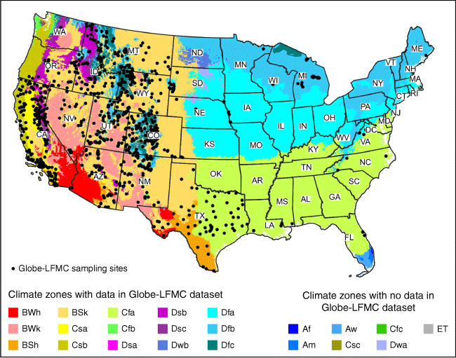
Climate zone data
The Köppen–Geiger climate classification system is derived from the work of Köppen (2011), and uses temperature and precipitation information to classify the Earth’s land surface into 30 climate zones (Kottek et al. 2006; Peel et al. 2007). The CONUS contains regions located in 22 of these climate zones (Fig. 1, see also Supplementary Material S1). The Köppen–Geiger climate zone dataset used in this study was generated from a model developed by Beck et al. (2018) that uses data from multiple independent climate data sources and accounts for topographic effects on climate (Roe 2005; McVicar et al. 2007). At 1 km (0.0083°) resolution, this is one of the higher-resolution Köppen–Geiger datasets available, capturing climate variability at a resolution close to that of the MODIS data.
|
Elevation data
The elevation data used in the results analysis are the NASA SRTM 30 m digital elevation data (NASA JPL 2013), which were obtained from GEE product USGS/SRTMGL1_003.
Data preparation
The Globe-LFMC samples used in this study are those collected from sites located across the CONUS and collected on or after 1 March 2002 – the earliest date that allows a 1-year time series of MODIS MCD43A4 data with a 1-year lead time to be obtained for each sample. There are 123 073 such samples collected from 932 sites. The LFMC samples were pre-processed by merging data collected on the same date from locations within the same MODIS pixel, which reduced the size of the dataset to 66 411 samples and 924 sites. The locations of these sites are shown in Fig. 1. Hereinafter, the terms Globe-LFMC dataset and LFMC samples refer to this pre-processed dataset, rather than the entire data collection.
Three static (auxiliary) variables were prepared for each sample: the latitude and longitude of the centroid of the MODIS pixel in which the sampling site is located, and climate zone at the pixel’s location. These variables were transformed to produce 18 normalised auxiliary variables, one representing the latitude, two representing the longitude and 15 representing the climate zone (one binary variable for each climate zone represented in the Globe-LFMC dataset). Full details of the normalisation and transformation processes are provided in Supplementary Material S2.
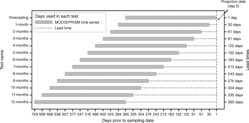
For every LFMC sample, and each lead time tested, 365-day by 1-pixel time series for both the MODIS and PRISM data were extracted from GEE. Each time series ends the specified ‘lead time’ days before the actual sampling date. Any gaps in the MODIS data were filled by linear interpolation of the surrounding time steps. Finally, the MODIS and PRISM time series were both normalised using the formula (bnmi − P2mi)/(P98mi − P2mi), where bnmi is the ith band of time series m (where m is either MODIS or PRISM) for sample n, and P2i and P98i are the 2nd and 98th percentile values extracted from the data for band bmi across all time steps and samples (Pelletier et al. 2019).
After pre-processing, the data for each sample consist of the measured LFMC (the target variable), a vector of 18 auxiliary variables, a 365-day × 7-spectral-band matrix of MODIS data, and a 365-day × 7-variable matrix of PRISM data.
Multi-tempCNN architecture
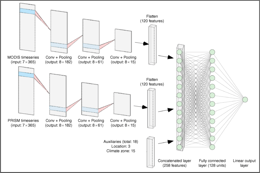
The Multi-tempCNN architecture (Miller et al. 2022) is a deep learning ensemble architecture designed for multi-modal inputs. Each singleton model in the ensemble uses the same architecture (Fig. 2) and is trained using the same data, but due to the stochastic deep learning process, produces different estimates for each exemplar. The final estimate is the mean of the estimates from the singleton models. The singleton models use a set of three one-dimensional convolutional layers to extract features from each of the time series inputs. These are followed by a fully connected layer that combines both sets of time series features with the auxiliary features using both linear and non-linear transformations to produce the output. Following Miller et al. (2022), an ensemble size of 20 is used.
|
Multi-tempCNN is based on a temporal convolutional neural network (tempCNN) originally developed for land cover classification (Pelletier et al. 2019). TempCNN was adapted for LFMC estimation by Zhu et al. (2021) and extended to multi-modal inputs and ensembling by Miller et al. (2022). The latter study considered two scenarios. The purpose of the first scenario was to make up-to-date LFMC estimates at sites with historical LFMC measurements; therefore, the models for this scenario were trained on historical data only and evaluated on the contemporaneous data. The purpose of the second (out-of-site) scenario was to simulate estimating LFMC at sites with no historical measurements. When evaluating model performance for this scenario, a set of sites were reserved as test sites. The models were trained using all the samples from the other sites and evaluated using the samples from the reserved test sites. In other words, each sample from the test sites was treated as if there were no historical LFMC data for the site. A key finding of Miller et al. (2022) was that different architectures benefitted each scenario. Because the aim of the current work is to evaluate the potential for Multi-tempCNN to make LFMC projections at unseen locations, the Multi-tempCNN architecture developed for out-of-site LFMC estimation has been used.
Evaluation methods
The code used to train and evaluate the nowcasting and projection models used in this study is a modified version of the code used to implement the original Multi-tempCNN models (Miller et al. 2022), and is available at https://github.com/lynn-miller/LFMC_estimation/tree/LFMC_projections. The code is written in Python (version 3.8) and uses Tensorflow v2.3 (Abadi et al. 2015) and Keras (Chollet et al. 2015).
Evaluation scenario
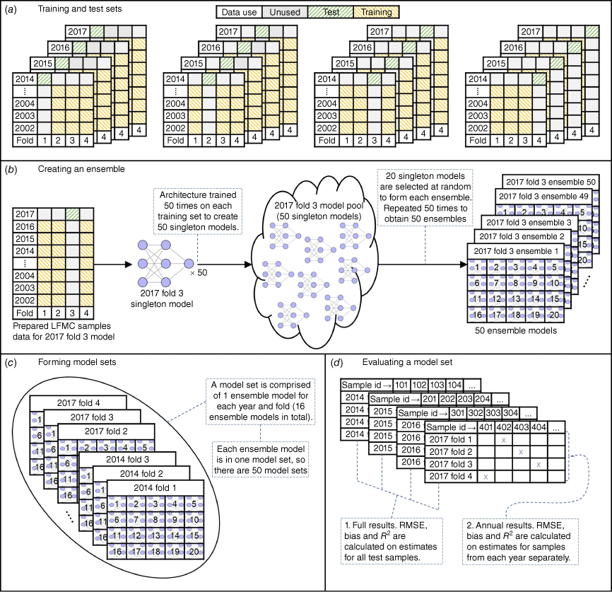
The evaluation scenario has been designed to (1) assess the generalisation capability of the model on unseen sites and (2) ensure the model used for making projections for a sample is trained using only data for samples collected prior to the sample in question, as would occur in practice. Therefore, in support of objective (1), each model is trained using data for samples from a subset of sites and tested using samples from the remaining sites. Sites are split into training and test sets using 4-fold cross-validation, with 25% of sites in each fold. Each fold is used in turn as the test set, with the other three folds forming the training set. In support of objective (2), each model is developed for use with only one evaluation year. Samples from the test sites for that year form the test set and samples for the training sites collected prior to that year form the training set. The evaluation years are 2014–2017 (the last four complete years in the Globe-LFMC dataset). This design with 4-fold cross validation across the physical sites for each of four evaluation years results in 16 sets of training and test data (Fig. 3a). The methodology is designed to ensure each model is evaluated on out of sample data and trained on data for samples collected prior to these evaluation samples, thus showing what the results would have been, if a prospective study had been conducted in each of the four evaluation years.
Ensembling method
The model for each of the 16 sets of training and test data comprises an ensemble (collection) of 20 singleton models, with the ensemble prediction being the mean of the singleton model predictions. To ensure robustness of the results, 50 models are constructed for each training and test set, and the evaluation metrics reported are averaged over the 50 models. However, because a naïve implementation of this would involve the creation of 16 000 singleton models for each test, the methodology used by Miller et al. (2022) is followed, in which a pool of 50 singleton models is created for each of the 16 training and test sets (Fig. 3b). Ensembles are formed by repeatedly selecting 20 of these singleton models at random for each ensemble. Thus, each test requires the significantly reduced number of 800 singleton models. Finally, the ensembled models are grouped into model sets, where each model set contains one ensembled model for each of the 16 training and test sets (Fig. 3c). Each ensembled model is in one model set, thus there are 50 model sets.
Evaluation metrics
The model performance was analysed using three metrics: (1) The root mean squared error (RMSE), which is calculated as  , where n is the number of samples and yi is the measured LFMC and
  the predicted LFMC for the ith sample; (2) the coefficient of determination (R2), which is defined as
  , where
  is the mean measured LFMC. When calculating R2 for a subset of samples, the mean LFMC used is that of the full sample set. This allows comparisons to be made between the R2 values for different sample subsets (Miller et al. 2022); and (3) the model bias, calculated as
  , indicates whether the model generally overpredicts (bias > 0) or underpredicts (bias < 0) LFMC. These metrics were calculated for each of the 50 model sets (Fig. 3d) separately to give 50 values. The mean and (where relevant) standard deviation of these 50 values are reported.
Analysis of model results over increasing lead times
In the first experiment, the model lead time was varied from 1 day (nowcasting model) to 1 year (365 days), in increments of 30 or 31 days (Fig. 4), resulting in 13 tests with approximately evenly spaced lead times. For convenience, the tests are referred to by the number of months in the lead time. This experiment assesses how the accuracy of the LFMC projections changes as the lead time increases. The results include the metrics for each of the four evaluation years, as well as for the entire test set (Fig. 3b).
Analysis of model results for 3-month LFMC projections
The purpose of this part of the evaluation is to analyse the projections made at a specific lead time, to understand where the projection models perform well and where they struggle. For this section, a projection lead time of 3 months was used, which is in line with seasonal climate forecasts (Ash et al. 2007; Weisheimer and Palmer 2014) and similar to seasonal fire risk predictions (Turco et al. 2019), while still having an accuracy acceptably close to the accuracy of comparable nowcasting studies (Zhu et al. 2021; Miller et al. 2022). The first sub-section of this analysis provides a further comparison between the 3-month projections and nowcasting estimates by examining key summary statistics. The remaining sub-sections analyse the 3-month projection results across different vegetation types and elevations, when fire danger is high or low, at varying levels of true LFMC, across different climate zones, and by geographic location.
Previous studies have found that forests, shrublands and grasslands respond differently to environmental factors so can have different moisture content given the same environmental conditions (Yebra et al. 2008; Nolan et al. 2022). Furthermore, vegetation cover changes at different elevations due to both physiological adaptation to the climate conditions (Brut et al. 2009) and differing species distribution (Allen et al. 1991), potentially presenting differing moisture profiles. For this reason, an analysis of model performance for (1) each land cover type and (2) land cover at various elevation ranges is included.
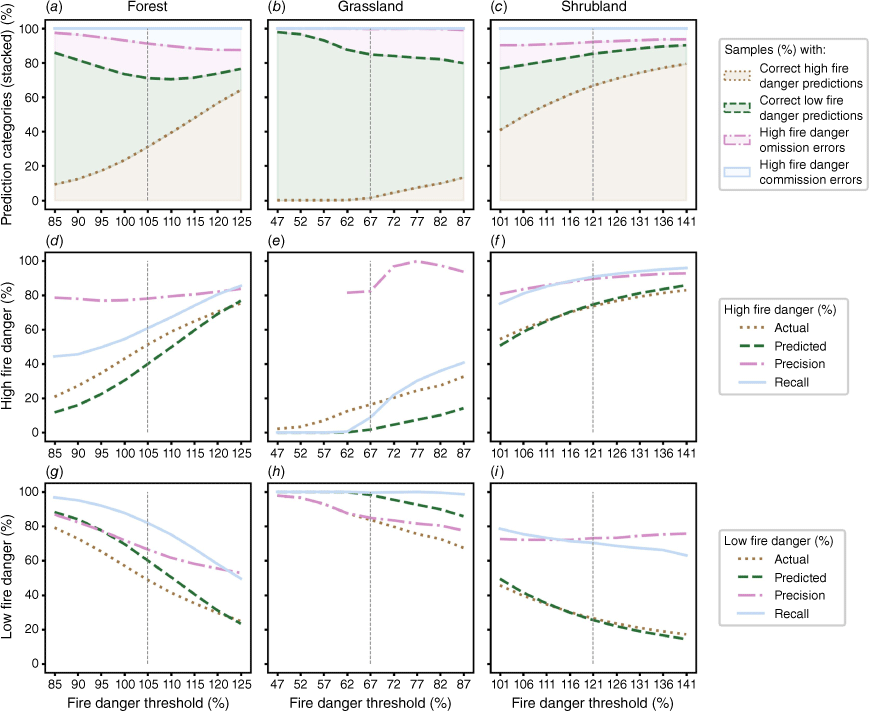
As important as good LFMC predictions across their full physical range are, if the projection model is to be useful for wildfire planning and management, good predictions are especially critical when LFMC is close to critical thresholds (Dennison and Moritz 2009), where fuels switch from a non-flammable to flammable state (herein referred to as fire danger thresholds or FDTs). Dry vegetation poses a high fire danger and small differences in LFMC predictions lead to large changes in perceived fire danger (Chuvieco et al. 2004). Therefore, the FDTs are used to identify the samples with a measured LFMC that indicates high fire danger, and the model performance is assessed using these samples. Various studies have proposed a range of thresholds (Chuvieco et al. 2004; Dennison et al. 2008; Jurdao et al. 2012; Argañaraz et al. 2018; Pimont et al. 2019). In this study, the FDTs used are those proposed by Argañaraz et al. (2018) because this is the only one of these aforementioned studies that established consistent thresholds across all the main vegetation types (forests, grasslands and shrublands). These thresholds, which are broadly in line with, but more conservative than, thresholds established by other studies, are 105% for forests, 67% for grasslands, and 121% for shrublands. Using these thresholds, the study (1) identifies the proportion of samples both correctly and incorrectly predicted as having a high or low fire danger and (2) provides performance metrics based on the model projections for the high fire danger samples in each land cover class. Because Argañaraz et al. (2018) studied pre-fire conditions in Argentina, there is some question about how useful their thresholds are for determining fire danger in the CONUS. Therefore, a threshold sensitivity study is also provided, showing how the model performs across a range of potential thresholds, from 20% below to 20% above each of the main thresholds, in increments of 5%. The study then investigates how model performance changes across ranges of ground-truth LFMC by grouping samples by measured LFMC into 5% intervals from 30 to 250%.
The spatial distribution of the Globe-LFMC sampling sites is skewed. The sites are located in only 15 of the 22 CONUS climate zones, and most are in the Csa (temperate climate with dry and hot summers) and BSk (arid, cold steppe) climate zones (Fig. 1), and in the western states. Therefore, two types of spatial analysis were performed to evaluate the potential of the model to generalise to climate zones and regions with few samples. Firstly, the RMSE, R2, and bias were computed for each climate zone using the LFMC projections for the samples collected from sites located within the climate zone. Secondly, changes in the projection performance across the CONUS were evaluated by grouping the sampling sites into 0.5° (latitude and longitude) grid cells, then computing the RMSE, R2, and bias of the LFMC projections for all samples collected from sites located within each cell.
LFMC maps
LFMC maps of the CONUS were produced for 1 April 2018 and 1 October 2018 using the 3-month projection model and the nowcasting model. The main purpose of these maps is to compare the predictions made by each model and demonstrate the projections are almost as accurate as the nowcasting model. Therefore, maps showing the differences between the projection and nowcasting maps are also provided. The map dates were chosen as being near the beginning and end of the wildfire season (Westerling et al. 2003; Swain 2021). The models used to produce the maps comprise an ensemble of 20 singleton models, with each model being trained using all the Globe-LFMC samples collected prior to 2018. Water bodies are identified and masked using the MODIS MOD44W.006 water mask product (Carroll et al. 2017).
Results
Analysis of model results over increasing lead times
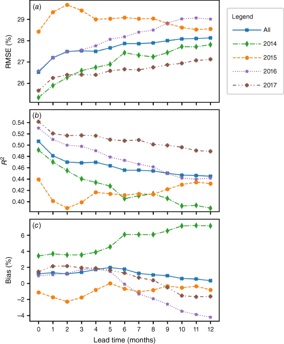
The model RMSE (Fig. 5a) initially increases comparatively quickly as the lead time is increased, from an RMSE of 26.52% for nowcasting (0-month lead time) to an RMSE of 27.52% for a 3-month lead time. It then increases slowly to 28.13% as the lead time is increased to 1 year. The model R2 (Fig. 5b), which is 0.51 for nowcasting, drops to 0.47 with a 3-month lead time and drops further to 0.44 with a 1-year lead time.
|
The results for each evaluation year follow different patterns. The overall trend is mirrored by the results for 2017, which consistently has an RMSE between 0.9 and 1.2% lower than the overall RMSE and an R2 0.05 higher. Both 2014 and 2016 show a more rapid increase in RMSE (and corresponding decrease in R2), which stabilises at about 10 months, although 2014 shows an anomalous increase at 6 and 7 months. The results for 2015 show a significant increase in RMSE over the 1–3-month lead times, before stabilising from 4 to 8 months, and then improving as the lead time increases to 1 year. The anomalous results for 2015 are likely due to the weather extremes experienced that year, including both extreme rainfall and temperatures (NOAA National Centers for Environmental Information 2016).
The overall bias (Fig. 5c) appears to improve as the lead time increases. However, this is due to an increasing positive bias for 2014 being offset by an increasing negative bias for 2016 and 2017. The high positive bias in 2014 mainly occurs in the predictions for samples collected between January and March, which may indicate the models did not fully anticipate the drought conditions in the south-western states (NOAA National Centers for Environmental Information 2014). The anomalous result for 2015 over the 1–3-month lead times is again seen in the bias, which drops to −2.28% before rising and stabilising at between 0 and −1.
Analysis of model results for 3-month LFMC projections
Nowcasting and 3-month projection comparison
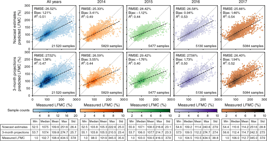
The evaluation samples have measured LFMC, which ranges from 1.0 to 434.5% (Fig. 6). The mean LFMC is 108.4% and the median is 102.7%, thus the dataset has a small right skew. The 3-month projection model predicts LFMC in the range of 53.7–274.7%. This is a slightly broader range than the estimates made by the nowcasting model (which ranges from 52.5 to 251.6%). The standard deviations of these predictions are 26.4% for the nowcasting model and 25.7% for the projection model, compared with a standard deviation of 37.8% for measured LFMC. The mean LFMC predicted by both models is close to that of the measured LFMC, but the medians are about 5% higher, indicating less skew in the predictions than in the measured values. Neither the nowcasting nor the projection models can predict extremely low or extremely high LFMC accurately; both tend to underpredict when LFMC is high and overpredict when it is low. This tendency is likely due to the small number of samples with field measured LFMC at the extremes, but the moderate to low resolution of the predictors may also be a factor.
Model performance by land cover and elevation
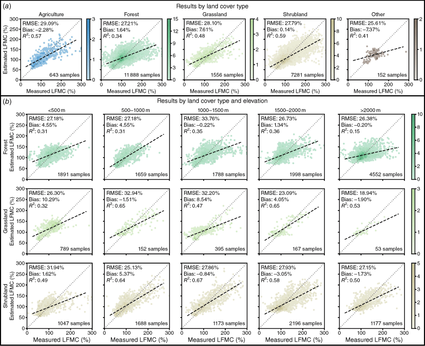
The RMSEs of the 3-month projections for the three main land cover classes are close to the overall RMSE, at 27.21% for forest, 27.79% for shrubland, and 28.10% for grassland (Fig. 7a). The R2 values show more variation between the classes than the RMSE values, at 0.34 for forest, 0.59 for shrubland and 0.48 for grassland. Thus, the models appear to cope well with the relatively high variance of measured LFMC in grasslands (Yebra et al. 2013). However, the model tends to overpredict grassland LFMC, with a bias of 7.61%. The forest results show a smaller bias of 1.64%, whereas there is almost no bias for shrubland results.
When the results for these land cover classes are broken down by elevation, there is a lot more variation in the performance (Fig. 7b). The best results for forest land cover are seen at 500–1000 m (RMSE is 21.59% and R2 is 0.64), and the poorest are at 1000–1500 m (RMSE 33.76% and R2 is 0.35). Although grassland appears to achieve good results for samples collected from above 2000 m, there are only 53 samples out of 5782 total samples at this elevation, so the results should be treated with caution. The best shrubland results are obtained at 500–1000 m (RMSE is 25.13% and R2 is 0.64), and the poorest are obtained at below 500 m (RMSE is 31.94% and R2 is 0.49). At elevations above 1000 m, shrubland RMSEs are close to the models’ overall RMSE.
Ability of the model to identify high fire danger conditions
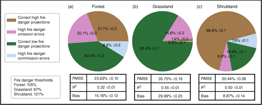
Each of the three main land cover classes has a different fire danger threshold (FDT) (Chuvieco et al. 2004), and therefore a different proportion of samples with a measured LFMC above and below the FDT. Using the indicative thresholds established by Argañaraz et al. (2018), grassland has a low FDT of 67%, and only 16% of the Globe-LFMC grassland samples have an LFMC below this threshold (Fig. 8b). This low threshold and small number of samples has resulted in a model that has poor recall when identifying grassland samples below the FDT, correctly identifying high fire danger in only 9% of the samples with an LFMC below the FDT. Forest has a higher FDT of 105%, and 52% of the forest samples have an LFMC below that threshold (Fig. 8a). Consequently, the model is better placed to identify high fire danger conditions in forest samples, with a recall of 61%. Shrubland has an even higher FDT of 121%, and 74% of shrubland samples have an LFMC below this threshold (Fig. 8c). The model identifies shrubland samples below the FDT with a recall of 91%.
Another way of viewing these results is to consider the model precision: if the model LFMC predictions are below the FDT, how likely is the measured LFMC to also be below the FDT. In other words, how confident can we be that the model has correctly identified high fire danger? For the forest samples, the model predicted 40% of the samples to have an LFMC below the forest FDT, with a precision of 78%; a similar analysis shows 67% precision in the low fire danger projections. The shrubland results show 90 and 73% precision in the samples with projected LFMC below and above the shrubland FDT, respectively. The grassland results show that although the model rarely predicted high fire danger, it was correct 82% of the time, and 85% of the substantial number of low fire danger LFMC projections for grassland samples were correct.
The performance metrics for the projections for forest and shrubland samples with high fire danger (tables below; Fig. 8a, c) provide further evidence that the model performs well. The RMSE for the forest samples showing high fire danger (23.63%) is well below the RMSE for all forest samples (27.21%), and the R2 value (0.32) is close to the R2 value for all the forest samples (0.34). The RMSE for the shrubland samples showing high fire danger (20.44%) is also well below the RMSE for all shrubland samples (27.79%). However, the R2 value (0.50) is also lower than the R2 value for all shrubland samples (0.59). The positive bias for both forest (15.16%) and shrublands (8.87%) shows the model tends to overpredict low LFMC, which could lead to omissions of high fire danger prediction, especially when LFMC is close to the FDT.
The RMSE for grassland samples with measured LFMC below the FDT (35.75%, table below; Fig. 8b) is well above the RMSE for all grassland samples (28.10%), and the projections have a positive bias (29.99%). However, the R2 is 0.55, which is well above the R2 for the full evaluation set (0.48), indicating a high degree of variability in LFMC for these grassland samples.
The FDT sensitivity study (Fig. 9) shows the model has low sensitivity to changes in the threshold used for shrublands, with the precision and recall for both high and low fire danger changing gradually over the range of thresholds tested. The model shows more sensitivity to the grassland threshold, due to small number of grassland samples with very low LFMC and the model’s difficulty predicting low LFMC values. This can be seen in the recall for high fire danger, which increases quickly as the threshold is increased. The model shows a mixture of sensitivity and robustness to the forest threshold. The high fire danger recall varies with the threshold (it drops if the threshold is lowered and increases if the threshold is raised). However, the precision is stable and the overall accuracy is above 70% for all thresholds tested.
|
Model performance by LFMC range
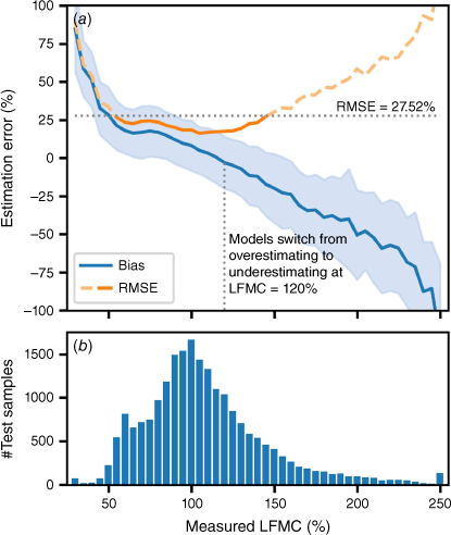
The projection model tends to overpredict LFMC when the measured value is low and underpredict when it is high (Fig. 10a), and switches from overpredicting to underpredicting when the measured LFMC is about 120%. The model clearly has difficulty making accurate projections when LFMC is extremely low or high, with high values for both the RMSE and the standard deviation of the projection error, probably due to the small number of samples (Fig. 10b). However, it performs well in the critical range of 50–120%, with RMSE below that of the full evaluation set, and the standard deviation of the projection error below 20%.
|
Model performance by climate zone
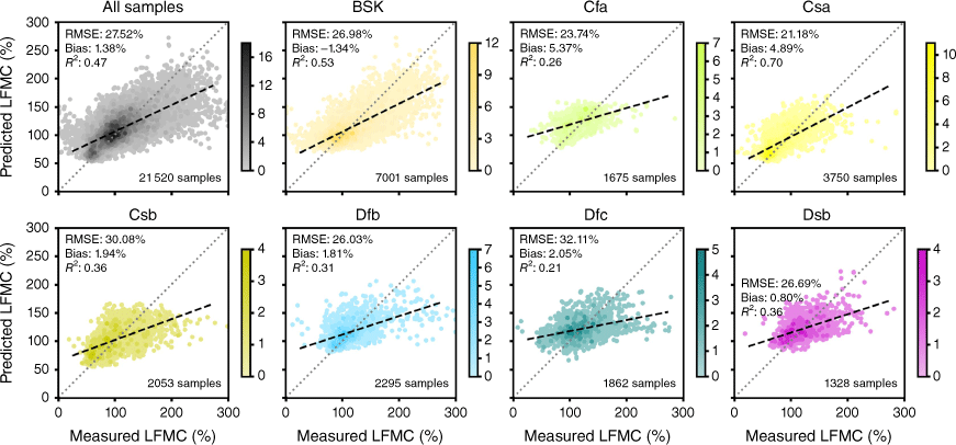
The analysis in this section considers the model performance across the seven climate zones that have more than 1000 evaluation samples (referred to here as the main climate zones). The other climate zones are not considered because they have too few evaluation samples and so results may not be reliable. Of the main climate zones, the model performed best on samples in the Csa climate zone (the Californian Mountain region), with an RMSE of 21.18% and R2 of 0.7 (Fig. 11). A good RMSE of 23.74% was also obtained on samples in the Cfa climate zone (which covers most of the south-eastern states, Fig. 1); however, the R2 value is also low – LFMC values for samples in this climate zone are tightly clustered around the sample mean. The main climate zones where the models performed the worst were Dfc (predominantly the Rocky Mountain regions of Colorado, Wyoming, and Montana) and Csb (the coastal regions of California, Oregon, and Washington states), with RMSEs of 32.11 and 30.08% and R2 values of 0.21 and 0.36, respectively. For samples in the other three main climate zones (Dsb, Dfb, and BSk), the model’s RMSEs were 26.69, 26.03, and 26.98%, respectively, so were below the overall RMSE of 27.52%.
Model performance by sampling site locations
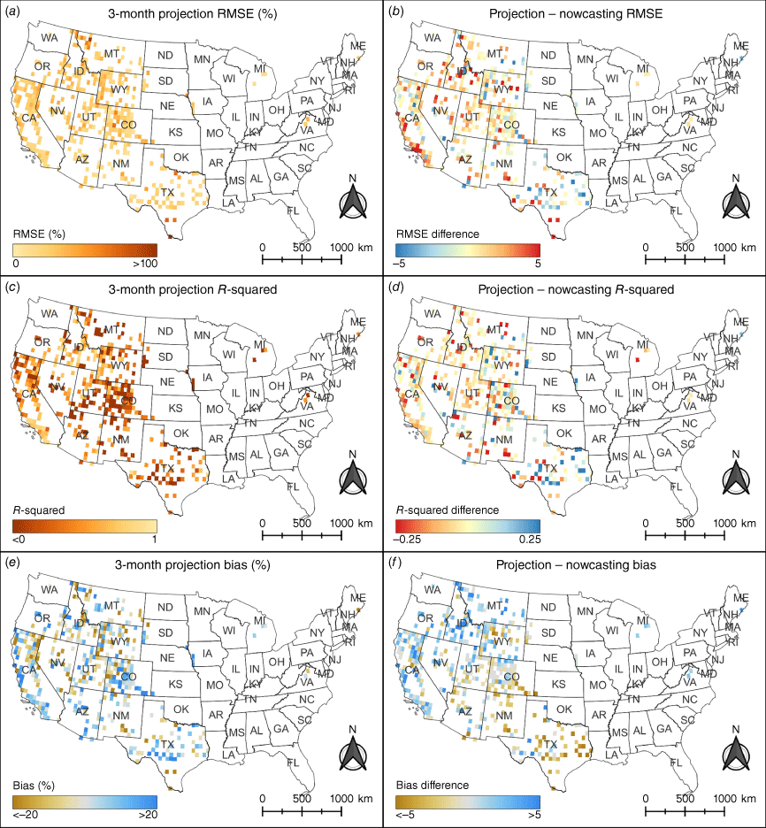
The RMSEs of the projection models’ predictions for the samples in each 0.5° grid cell ranged from 4.32 to 111.68%, with a median RMSE of 23.92% (Fig. 12a). This is similar to the RMSEs of the nowcasting models, which ranged from 4.60 to 102.54%, with a median of 23.72%. In 60% of the grid cells, the projection RMSE differed by less than 5% from the nowcasting RMSE (Fig. 12b), and in another 36% of grid cells the projection RMSE was lower than the nowcasting RMSE. The projection median R2 value for the grid cells is 0.36 (Fig. 12c), which is slightly lower than the nowcasting median (0.39, Fig. 12d). Although the R2 values for both the projection and nowcasting models were less than zero for a sizeable number of the grid cells, these are mainly cells with few samples and/or low variance.
The projection models overpredicted LFMC in 51% of the grid cells (Fig. 12e), which is slightly less than the nowcasting models (52%). Compared with the nowcasting estimates, the projection models predicted drier vegetation in the southern and central states of Texas (TX), New Mexico (NM), and Colorado (CO) (Fig. 12f). Wetter vegetation can be observed in California (CA), Idaho (ID), and Montana (MT).
LFMC maps
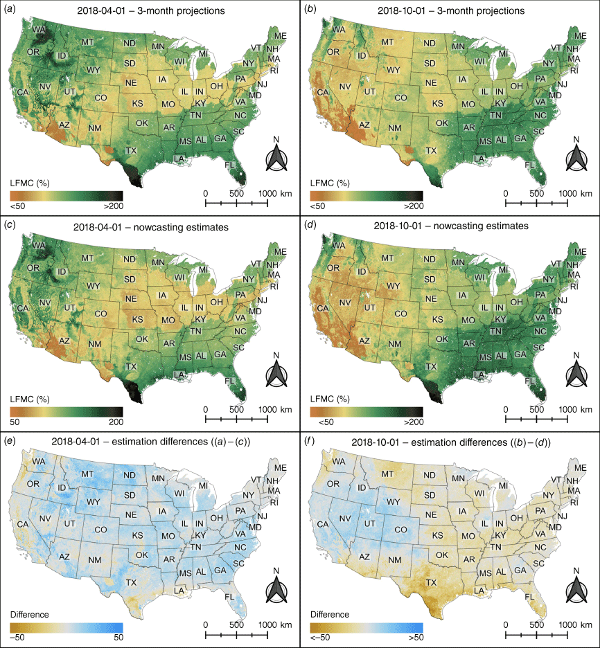
The 3-month projection maps for both 1 April 2018 and 1 October 2018 (Fig. 13a, b) are very similar to the respective nowcasting maps (Fig. 13c, d). For April, the absolute difference between the nowcasting and 3-month projection LFMC predictions was less than 10% for 71% of the pixels. The projections were lower than the nowcasting estimates in the western coastal areas and southern Texas (Fig. 13e), where the projection model may have been unduly influenced by the drier and hotter than average weather these regions experienced in 2017 (NOAA National Centers for Environmental Information 2018a), but higher in most eastern states and the western states of Idaho, Montana, Wyoming, and North Dakota. The October nowcasting and 3-month projection LFMC predictions had an absolute difference of less than 10% for 81% of the pixels. The LFMC projections were generally higher than the nowcasting estimates in western states (Fig. 13f) and lower in the southern and central states. A prominent area of lower LFMC prediction can be seen in Texas, possibly indicating the projection model did not anticipate the higher than average summer precipitation in this region (NOAA National Centers for Environmental Information 2018b).
Comparison of the April and October LFMC projections show clear differences. Generally, projected vegetation moisture levels were higher in April (median projected LFMC was 118%) than October (median projected LFMC was 108%). However, differences across the CONUS can be seen. The lower October LFMC projections occur mainly in the western states (median LFMC reduces from 116 to 101%), which predominantly have arid climate or dry summers; whereas eastern states, which have wetter summers, have higher LFMC in October (median LFMC increases from 119 to 130%).
Discussion
This study introduces a novel method to make reasonably accurate projections of LFMC 3 months in advance, using the Multi-tempCNN deep learning architecture. This architecture is designed for moderate resolution (500 m) LFMC predictions at continental scales and requires no prior knowledge of the vegetation type (Miller et al. 2022). The model performance was only slightly less accurate than the performance of the nowcasting model, with RMSE increasing from 26.5 to 27.5% and R2 decreasing from 0.51 to 0.47. To the best of our knowledge, this study is the first to present a wide-scale model projecting LFMC with more than a 14-day lead time.
These results are all the more encouraging considering the evaluation scenario presents a harder challenge than that used in many nowcasting studies. Our evaluation tests the capability of the model to generalise to both unseen sites and to future dates, whereas scenarios used in other studies only consider one of these generalisations per scenario. Rao et al. (2020) only considers generalisation to unseen sites, and both Zhu et al. (2021) and Miller et al. (2022) consider these two generalisations in separate scenarios.
The projection model predicts LFMC based on trends and seasonal information contained in the remote sensing and meteorological data. However, due to the 3-month lead time, the model does not have information about short term local weather patterns that occur close to the prediction date. Therefore, short-term anomalous weather can lead to changes in LFMC (Fox-Hughes et al. 2021) that cannot be anticipated by the projection model; it is therefore a source of uncertainty in the projections that should be taken into consideration when using the model results.
Another potential source of uncertainty comes from the low to moderate spatial resolution of the predictors (4 km for PRISM and 500 m for MODIS). This may be addressable in part in future work, by replacing the MODIS data with data from a higher spatial resolution source such as the Multi Spectral Instrument on board the Sentinel-2 satellites (European Space Agency 2019) – which has 20 m spatial resolution in the shortwave-infrared frequencies, but only 5-day temporal resolution – once sufficient more-recent ground-truth LFMC data are available.
The 3-month projection capability of Multi-tempCNN was analysed across different vegetation types, including at different elevations and when fire danger is high or low. The results showed consistency across the main land cover groups of forest, grassland and shrubland, and when adequate samples are available, at various elevations. However, results were more mixed when samples indicating high and low fire danger were considered separately. Analysis using the FDT determined by Argañaraz et al. (2018) showed the model was able to distinguish between high and low fire danger in both forest and shrubland samples, and made good LFMC projections for the high fire danger samples from both groups. However, the model did not perform as well on high fire danger grassland samples, substantially overpredicting the LFMC of these samples. This is due to both the low grassland FDT and the small number of grassland samples with LFMC below the FDT; consequently, most of these samples have LFMCs in the range where the model is known to overpredict LFMC.
The FDT used were established from a study in Argentina (Argañaraz et al. 2018), and so may have limited applicability to the CONUS. Although this is a limitation of the study, the issue has been addressed in part by providing a threshold sensitivity analysis, showing how the model performs at a range of thresholds. This analysis showed shrubland results were reasonably insensitive to the threshold used, whereas the forest results showed more sensitivity. The grassland results were quite sensitive to the threshold, again due to the small number of grassland samples with LFMC at or below the thresholds tested.
The small decrease in performance of the projection model from state-of-the-art nowcasting models shows that deep learning models have good capability for LFMC projections. However, there is a need for further improvements, particularly for grasslands under high fire danger conditions. Additionally, the evaluation by climate zone shows the model performs better in regions that have stable seasonal weather patterns. Finally, the model has no information about expected changes to vegetation conditions during the 3-month lead time, which could be provided by the incorporation of long-range weather or climate anomaly forecast data into the model. Future work includes evaluating the effect of adding this forecast data into the model, extending the model to non-CONUS regions, and incorporating uncertainty estimation techniques into the model.
Supplementary material
Supplementary material is available online.
Data availability
All datasets used in this study are either open access or free for non-commercial usage. These datasets are listed in Table 1, together with the reference to the creator, license details and link to the source used in this study.

|
Conflicts of interest
The authors declare no conflicts of interest.
Declaration of funding
This work was supported by an Australian Government Research Training Program (RTP) scholarship and the Australian Research Council under award DP210100072.
Acknowledgements
We thank the Associate Editor and reviewer for their helpful and constructive comments and feedback. The diagram of the Multi-tempCNN model shown in Fig. 2 was created with the help of Alexander LeNail’s NN-SVG webpage (https://alexlenail.me/NN-SVG/index.html). All maps were created using QGIS version 3.22 (https://qgis.org/en/site/).
References
Abadi M, Agarwal A, Barham P, Brevdo E, Chen Z, Citro C, Corrado GS, Davis A, Dean J, Devin M, Ghemawat S, Goodfellow I, Harp A, Irving G, Isard M, Jia Y, Jozefowicz R, Kaiser L, Kudlur M, Levenberg J, Mané D, Monga R, Moore S, Murray D, Olah C, Schuster M, Shlens J, Steiner B, Sutskever I, Talwar K, Tucker P, Vanhoucke V, Vasudevan V, Viégas F, Vinyals O, Warden P, Wattenberg M, Wicke M, Yu Y, Zheng X, Google Research (2015) TensorFlow: large-scale machine learning on heterogeneous distributed systems. Available at www.tensorflow.orgAllen RB, Peet RK, Baker WL (1991) Gradient analysis of latitudinal variation in southern Rocky Mountain forests. Journal of Biogeography 18, 123–139.
| Gradient analysis of latitudinal variation in southern Rocky Mountain forests.Crossref | GoogleScholarGoogle Scholar |
Argañaraz JP, Landi MA, Scavuzzo CM, Bellis LM (2018) Determining fuel moisture thresholds to assess wildfire hazard: a contribution to an operational early warning system. PLoS One 13, e0204889
| Determining fuel moisture thresholds to assess wildfire hazard: a contribution to an operational early warning system.Crossref | GoogleScholarGoogle Scholar |
Ash A, McIntosh P, Cullen B, Carberry P, Smith MS (2007) Constraints and opportunities in applying seasonal climate forecasts in agriculture. Australian Journal of Agricultural Research 58, 952–965.
| Constraints and opportunities in applying seasonal climate forecasts in agriculture.Crossref | GoogleScholarGoogle Scholar |
Beck HE, Zimmermann NE, McVicar TR, Vergopolan N, Berg A, Wood EF (2018) Present and future Köppen–Geiger climate classification maps at 1-km resolution. Scientific Data 5, 180214
| Present and future Köppen–Geiger climate classification maps at 1-km resolution.Crossref | GoogleScholarGoogle Scholar |
Bedia J, Golding N, Casanueva A, Iturbide M, Buontempo C, Gutiérrez JM (2018) Seasonal predictions of Fire Weather Index: paving the way for their operational applicability in Mediterranean Europe. Climate Services 9, 101–110.
| Seasonal predictions of Fire Weather Index: paving the way for their operational applicability in Mediterranean Europe.Crossref | GoogleScholarGoogle Scholar |
Brut A, Rüdiger C, Lafont S, Roujean J-L, Calvet J-C, Jarlan L, Gibelin A-L, Albergel C, Le Moigne P, Soussana J-F, Klumpp K, Guyon D, Wigneron J-P, Ceschia E (2009) Modelling LAI at a regional scale with ISBA-A-gs: comparison with satellite-derived LAI over southwestern France. Biogeosciences 6, 1389–1404.
| Modelling LAI at a regional scale with ISBA-A-gs: comparison with satellite-derived LAI over southwestern France.Crossref | GoogleScholarGoogle Scholar |
Buban MS, Lee TR, Baker CB (2020) A comparison of the U.S. Climate Reference Network precipitation data to the Parameter–Elevation Regressions on Independent Slopes Model (PRISM). Journal of Hydrometeorology 21, 2391–2400.
| A comparison of the U.S. Climate Reference Network precipitation data to the Parameter–Elevation Regressions on Independent Slopes Model (PRISM).Crossref | GoogleScholarGoogle Scholar |
Carroll M, DiMiceli C, Wooten M, Hubbard A, Sohlberg R, Townshend J (2017) MOD44W MODIS/Terra Land Water Mask Derived from MODIS and SRTM L3 Global 250m SIN Grid V006. United States Geological Survey, Sioux Falls, SD, USA.
| Crossref |
Catchpole E, Catchpole W (1991) Modelling moisture damping for fire spread in a mixture of live and dead fuels. International Journal of Wildland Fire 1, 101–106.
| Modelling moisture damping for fire spread in a mixture of live and dead fuels.Crossref | GoogleScholarGoogle Scholar |
Chollet F, et al. (2015) Keras. Available at https://keras.io
Chuvieco E, Aguado I, Dimitrakopoulos AP (2004) Conversion of fuel moisture content values to ignition potential for integrated fire danger assessment. Canadian Journal of Forest Research 34, 2284–2293.
| Conversion of fuel moisture content values to ignition potential for integrated fire danger assessment.Crossref | GoogleScholarGoogle Scholar |
Chuvieco E, Aguado I, Salas J, García M, Yebra M, Oliva P (2020) Satellite remote sensing contributions to wildland fire science and management. Current Forestry Reports 6, 81–96.
| Satellite remote sensing contributions to wildland fire science and management.Crossref | GoogleScholarGoogle Scholar |
Daly C, Halbleib M, Smith JI, Gibson WP, Doggett MK, Taylor GH, Curtis J, Pasteris PP (2008) Physiographically sensitive mapping of climatological temperature and precipitation across the conterminous United States. International Journal of Climatology 28, 2031–2064.
| Physiographically sensitive mapping of climatological temperature and precipitation across the conterminous United States.Crossref | GoogleScholarGoogle Scholar |
Daly C, Smith JI, Olson KV (2015) Mapping atmospheric moisture climatologies across the conterminous United States. PLoS One 10, e0141140
| Mapping atmospheric moisture climatologies across the conterminous United States.Crossref | GoogleScholarGoogle Scholar |
Danson FM, Bowyer P (2004) Estimating live fuel moisture content from remotely sensed reflectance. Remote Sensing of Environment 92, 309–321.
| Estimating live fuel moisture content from remotely sensed reflectance.Crossref | GoogleScholarGoogle Scholar |
Dasgupta S, Qu J, Hao X, Bhoi S (2007) Evaluating remotely sensed live fuel moisture estimations for fire behavior predictions in Georgia, USA. Remote Sensing of Environment 108, 138–150.
| Evaluating remotely sensed live fuel moisture estimations for fire behavior predictions in Georgia, USA.Crossref | GoogleScholarGoogle Scholar |
Dennison PE, Moritz MA (2009) Critical live fuel moisture in chaparral ecosystems: a threshold for fire activity and its relationship to antecedent precipitation. International Journal of Wildland Fire 18, 1021–1027.
| Critical live fuel moisture in chaparral ecosystems: a threshold for fire activity and its relationship to antecedent precipitation.Crossref | GoogleScholarGoogle Scholar |
Dennison PE, Moritz MA, Taylor RS (2008) Evaluating predictive models of critical live fuel moisture in the Santa Monica Mountains, California. International Journal of Wildland Fire 17, 18–27.
| Evaluating predictive models of critical live fuel moisture in the Santa Monica Mountains, California.Crossref | GoogleScholarGoogle Scholar |
Dimitrakopoulos AP, Papaioannou KK (2001) Flammability assessment of Mediterranean forest fuels. Fire Technology 37, 143–152.
| Flammability assessment of Mediterranean forest fuels.Crossref | GoogleScholarGoogle Scholar |
European Space Agency (2019) Sentinel Online. European Space Agency, Paris, France. Available at https://sentinel.esa.int/web/sentinel/home
Fox-Hughes P, Yebra M, Kumar V, Dowdy AJ, Hope P, Peace M, Narsey S, Shokirov S, Delage F, Zhang H (2021) Soil and fuel moisture precursors of fire activity during the 2019-20 fire season, in comparison to previous seasons. Bushfire and Natural Hazards CRC, Melbourne, Vic., Australia. Available at https://www.naturalhazards.com.au/research/research-projects/soil-and-fuel-moisture-precursors-fire-activity-during-2019-20-fire
Gorelick N, Hancher M, Dixon M, Ilyushchenko S, Thau D, Moore R (2017) Google Earth Engine: planetary-scale geospatial analysis for everyone. Remote Sensing of Environment 202, 18–27.
| Google Earth Engine: planetary-scale geospatial analysis for everyone.Crossref | GoogleScholarGoogle Scholar |
Jackson TJ (1993) III. Measuring surface soil moisture using passive microwave remote sensing. Hydrological Processes 7, 139–152.
| III. Measuring surface soil moisture using passive microwave remote sensing.Crossref | GoogleScholarGoogle Scholar |
Jia S, Kim SH, Nghiem SV, Kafatos M (2019) Estimating live fuel moisture using SMAP L-band radiometer soil moisture for Southern California, USA. Remote Sensing 11, 1575
| Estimating live fuel moisture using SMAP L-band radiometer soil moisture for Southern California, USA.Crossref | GoogleScholarGoogle Scholar |
Jurdao S, Chuvieco E, Arevalillo JM (2012) Modelling fire ignition probability from satellite estimates of live fuel moisture content. Fire Ecology 8, 77–97.
| Modelling fire ignition probability from satellite estimates of live fuel moisture content.Crossref | GoogleScholarGoogle Scholar |
Konings AG, Rao K, Steele‐Dunne SC (2019) Macro to micro: microwave remote sensing of plant water content for physiology and ecology. New Phytologist 223, 1166–1172.
| Macro to micro: microwave remote sensing of plant water content for physiology and ecology.Crossref | GoogleScholarGoogle Scholar |
Köppen W (2011) The thermal zones of the Earth according to the duration of hot, moderate and cold periods and to the impact of heat on the organic world. Meteorologische Zeitschrift 20, 351–360.
| The thermal zones of the Earth according to the duration of hot, moderate and cold periods and to the impact of heat on the organic world.Crossref | GoogleScholarGoogle Scholar |
Kottek M, Grieser J, Beck C, Rudolf B, Rubel F (2006) World map of the Köppen–Geiger climate classification updated. Meteorologische Zeitschrift 15, 259–263.
| World map of the Köppen–Geiger climate classification updated.Crossref | GoogleScholarGoogle Scholar |
Lu Y, Wei C (2021) Evaluation of microwave soil moisture data for monitoring live fuel moisture content (LFMC) over the coterminous United States. Science of the Total Environment 771, 145410
| Evaluation of microwave soil moisture data for monitoring live fuel moisture content (LFMC) over the coterminous United States.Crossref | GoogleScholarGoogle Scholar |
Marino E, Yebra M, Guillén-Climent M, Algeet N, Tomé JL, Madrigal J, Guijarro M, Hernando C (2020) Investigating live fuel moisture content estimation in fire-prone shrubland from remote sensing using empirical modelling and RTM simulations. Remote Sensing 12, 2251
| Investigating live fuel moisture content estimation in fire-prone shrubland from remote sensing using empirical modelling and RTM simulations.Crossref | GoogleScholarGoogle Scholar |
McVicar TR, Van Niel TG, Li L, Hutchinson MF, Mu X, Liu Z (2007) Spatially distributing monthly reference evapotranspiration and pan evaporation considering topographic influences. Journal of Hydrology 338, 196–220.
| Spatially distributing monthly reference evapotranspiration and pan evaporation considering topographic influences.Crossref | GoogleScholarGoogle Scholar |
Miller L, Zhu L, Yebra M, Rüdiger C, Webb GI (2022) Multi-modal temporal CNNs for live fuel moisture content estimation. Environmental Modelling & Software 156, 105467
| Multi-modal temporal CNNs for live fuel moisture content estimation.Crossref | GoogleScholarGoogle Scholar |
NASA JPL (2013) NASA Shuttle Radar Topography Mission Global 1 arc second. United States Geological Survey, Sioux Falls, SD, USA.
| Crossref |
NOAA National Centers for Environmental Information (2014) State of the Climate: Monthly National Climate Report for March 2014. National Centers for Environmental Information, Asheville, NC, USA. Available at https://www.ncei.noaa.gov/access/monitoring/monthly-report/national/201403
NOAA National Centers for Environmental Information (2016) State of the Climate: National Climate Report for Annual 2015. National Centers for Environmental Information, Asheville, NC, USA. Available at https://www.ncdc.noaa.gov/sotc/national/201513
NOAA National Centers for Environmental Information (2018a) National Temperature and Precipitation Maps, 2017 anomalies. National Centers for Environmental Information, Asheville, NC, USA. Available at https://www.ncei.noaa.gov/access/monitoring/us-maps/ytd/201712?products[]=tmax-anom&products[]=tmin-anom&products[]=tave-anom&products[]=prcp-diff
NOAA National Centers for Environmental Information (2018b) National Temperature and Precipitation Maps, July – September 2018 anomalies. National Centers for Environmental Information, Asheville, NC, USA. Available at https://www.ncei.noaa.gov/access/monitoring/us-maps/3/201809?products[]=tmax-anom&products[]=tmin-anom&products[]=tave-anom&products[]=prcp-diff
Nolan RH, Foster B, Griebel A, Choat B, Medlyn BE, Yebra M, Younes N, Boer MM (2022) Drought-related leaf functional traits control spatial and temporal dynamics of live fuel moisture content. Agricultural and Forest Meteorology 319, 108941
| Drought-related leaf functional traits control spatial and temporal dynamics of live fuel moisture content.Crossref | GoogleScholarGoogle Scholar |
Park I, Fauss K, Moritz MA (2022) Forecasting live fuel moisture of Adenostema fasciculatum and its relationship to regional wildfire dynamics across Southern California shrublands. Fire 5, 110
| Forecasting live fuel moisture of Adenostema fasciculatum and its relationship to regional wildfire dynamics across Southern California shrublands.Crossref | GoogleScholarGoogle Scholar |
Peel MC, Finlayson BL, McMahon TA (2007) Updated world map of the Köppen–Geiger climate classification. Hydrology and Earth System Sciences 11, 1633–1644.
| Updated world map of the Köppen–Geiger climate classification.Crossref | GoogleScholarGoogle Scholar |
Pelletier C, Webb G, Petitjean F (2019) Temporal convolutional neural network for the classification of satellite image time series. Remote Sensing 11, 523
| Temporal convolutional neural network for the classification of satellite image time series.Crossref | GoogleScholarGoogle Scholar |
Pimont F, Ruffault J, Martin-StPaul NK, Dupuy J-L (2019) Why is the effect of live fuel moisture content on fire rate of spread underestimated in field experiments in shrublands? International Journal of Wildland Fire 28, 127–137.
| Why is the effect of live fuel moisture content on fire rate of spread underestimated in field experiments in shrublands?Crossref | GoogleScholarGoogle Scholar |
Rao K, Williams AP, Flefil JF, Konings AG (2020) SAR-enhanced mapping of live fuel moisture content. Remote Sensing of Environment 245, 111797
| SAR-enhanced mapping of live fuel moisture content.Crossref | GoogleScholarGoogle Scholar |
Roe GH (2005) Orographic precipitation. Annual Review of Earth and Planetary Sciences 33, 645–671.
| Orographic precipitation.Crossref | GoogleScholarGoogle Scholar |
Schaaf C, Wang Z (2015) MCD43A4 MODIS/Terra+Aqua BRDF/Albedo Nadir BRDF-Adjusted Ref Daily L3 Global 500m V006. NASA EOSDIS L. Process. DAAC. United States Geological Survey, Sioux Falls, SD, USA.
| Crossref |
Sharma S, Dhakal K (2021) Boots on the ground and eyes in the sky: a perspective on estimating fire danger from soil moisture content. Fire 4, 45
| Boots on the ground and eyes in the sky: a perspective on estimating fire danger from soil moisture content.Crossref | GoogleScholarGoogle Scholar |
Strahler A, Gopal S, Lambin E, Moody A (1999) MODIS Land Cover Product Algorithm Theoretical Basis Document (ATBD) MODIS Land Cover and Land-Cover Change. National Aeronautics and Space Administration, Washington, DC, USA. Available at http://modis.gsfc.nasa.gov/data/atbd/atbd_mod12.pdf
Swain DL (2021) A shorter, sharper rainy season amplifies California wildfire risk. Geophysical Research Letters 48, e2021GL092843
| A shorter, sharper rainy season amplifies California wildfire risk.Crossref | GoogleScholarGoogle Scholar |
Turco M, Marcos-Matamoros R, Castro X, Canyameras E, Llasat MC (2019) Seasonal prediction of climate-driven fire risk for decision-making and operational applications in a Mediterranean region. Science of the Total Environment 676, 577–583.
| Seasonal prediction of climate-driven fire risk for decision-making and operational applications in a Mediterranean region.Crossref | GoogleScholarGoogle Scholar |
Vinodkumar V, Dharssi I, Yebra M, Fox-Hughes P (2021) Continental-scale prediction of live fuel moisture content using soil moisture information. Agricultural and Forest Meteorology 307, 108503
| Continental-scale prediction of live fuel moisture content using soil moisture information.Crossref | GoogleScholarGoogle Scholar |
Walton D, Hall A (2018) An assessment of high-resolution gridded temperature datasets over California. Journal of Climate 31, 3789–3810.
| An assessment of high-resolution gridded temperature datasets over California.Crossref | GoogleScholarGoogle Scholar |
Weisheimer A, Palmer TN (2014) On the reliability of seasonal climate forecasts. Journal of the Royal Society Interface 11, 20131162
| On the reliability of seasonal climate forecasts.Crossref | GoogleScholarGoogle Scholar |
Westerling AL, Gershunov A, Brown TJ, Cayan DR, Dettinger MD (2003) Climate and wildfire in the Western United States. Bulletin of the American Meteorological Society 84, 595–604.
| Climate and wildfire in the Western United States.Crossref | GoogleScholarGoogle Scholar |
Yebra M, Chuvieco E, Riaño D (2008) Estimation of live fuel moisture content from MODIS images for fire risk assessment. Agricultural and Forest Meteorology 148, 523–536.
| Estimation of live fuel moisture content from MODIS images for fire risk assessment.Crossref | GoogleScholarGoogle Scholar |
Yebra M, Dennison PE, Chuvieco E, Riaño D, Zylstra P, Hunt ER, Danson FM, Qi Y, Jurdao S (2013) A global review of remote sensing of live fuel moisture content for fire danger assessment: moving towards operational products. Remote Sensing of Environment 136, 455–468.
| A global review of remote sensing of live fuel moisture content for fire danger assessment: moving towards operational products.Crossref | GoogleScholarGoogle Scholar |
Yebra M, Quan X, Riaño D, Rozas Larraondo P, van Dijk AIJM, Cary GJ (2018) A fuel moisture content and flammability monitoring methodology for continental Australia based on optical remote sensing. Remote Sensing of Environment 212, 260–272.
| A fuel moisture content and flammability monitoring methodology for continental Australia based on optical remote sensing.Crossref | GoogleScholarGoogle Scholar |
Yebra M, Scortechini G, Badi A, Beget ME, Boer MM, Bradstock R, Chuvieco E, Danson FM, Dennison P, Resco de Dios V, Di Bella CM, Forsyth G, Frost P, Garcia M, Hamdi A, He B, Jolly M, Kraaij T, Martín MP, Mouillot F, Newnham G, Nolan RH, Pellizzaro G, Qi Y, Quan X, Riaño D, Roberts D, Sow M, Ustin S (2019) Globe-LFMC, a global plant water status database for vegetation ecophysiology and wildfire applications. Scientific Data 6, 155
| Globe-LFMC, a global plant water status database for vegetation ecophysiology and wildfire applications.Crossref | GoogleScholarGoogle Scholar |
Zhu L, Webb GI, Yebra M, Scortechini G, Miller L, Petitjean F (2021) Live fuel moisture content estimation from MODIS: a deep learning approach. ISPRS Journal of Photogrammetry and Remote Sensing 179, 81–91.
| Live fuel moisture content estimation from MODIS: a deep learning approach.Crossref | GoogleScholarGoogle Scholar |


