

Developing an impact index for the Australian Fire Danger Rating System: predicting potential structure loss from wildfires
Dan Krix A , James Monks A , Stuart Matthews C , Meaghan Jenkins A B * , Alex Holmes A , Sam Sauvage D and John W. Runcie A
A
B
C
D
Abstract
Accurately predicting impacts of wildfires remains a top priority for fire and land management agencies. The Australian Fire Danger Rating System (AFDRS) redesigned forecasts of fire danger for Australian fire agencies, modernising the fire danger system. The next phase of the AFDRS focuses on developing indices for Fire Ignition, Suppression and Impact (FISI).
Impact models were developed to predict structure loss at the bushland–urban interface in eastern Australia.
Structure counts, cleared land and canopy height, calculated at radii 50–1000 m from structures, as well as terrain ruggedness, were used to model individual structure loss during wildfire and proportional loss in built-up areas.
The individual and proportional structure loss models accurately predicted structure loss (individual losses: true positive rate (TPR) = 0.67, true negative rate (TNR) = 0.69; proportional loss r2 = 0.71). Loss was lowest where structures had defensible space on flat ground, with higher numbers of structures nearby and shorter vegetation canopy height.
The models determine the probability of structure loss during destructive wildfire.
These models provide fire agencies information on the likelihood of structure loss and aid in decision-making. The impact index may support effective resource allocation, potentially reducing structure loss.
Keywords: AFDRS, fire danger rating, forecast, impact, model, probability, structure loss, wildfire.
Introduction
Wildfires and their potential impacts on life and property are becoming increasingly complex and uncertain. This can be attributed in part to the interactions between fire behaviour, increasing populations at the wildfire interface, variations in land-use, community preparedness levels (Whittaker and Clark 2021) and awareness and response to warnings (Strahan 2020; Whittaker et al. 2020). Globally, changes in land-use and climate processes have altered fire regimes, trending toward larger and higher-severity fires (Nolan et al. 2022) with enhanced overnight fire activity and multi-day fire events (Peace and McCaw 2024). Despite this increasing complexity and uncertainty, developing accurate predictions of the future impacts of wildfires remains a high priority for fire and land management agencies.
House loss by wildfire has been associated with the loss of life (Blanchi et al. 2012, 2014), with most fatalities associated with wildfires in Australia occurring among people evacuating from, sheltering in, or defending houses (Haynes et al. 2010). There are clear geographical trends in fatalities around population centres in south-eastern Australia, suggesting population density and/or housing density as key factors (Haynes et al. 2010; Blanchi et al. 2014). Accurately predicting house losses on a scale that informs decision-making for preparedness and planning to reduce house loss and improve human safety is needed; many current models predicting house loss have been developed at a resolution of 10s of metres and focus on localised or fine scale (individual structure) dynamics (Blanchi et al. 2006; Opie et al. 2014, Gibbons et al. 2018). These models have primarily been developed using large-scale events associated with large numbers of house losses under extreme fire weather behaviour, such as Ash Wednesday and Black Saturday in Victoria (Wilson and Ferguson 1986; Harris et al. 2011, 2012; Kilinc et al. 2013; Duff et al. 2019).
Other approaches have made use of successive runs of fire simulation programs, intended to delineate areas where fire and built-up areas are predicted to intersect (Massada et al. 2009; Ager et al. 2021). Deviations from normal weather patterns or heightened fire activity have also been used in actuarial models to model risk aggregated over large areas (Raveendran et al. 2024). Generally, studies are conducted at a fine spatial scale (metres), which is suited for risk planning (Tolhurst et al. 2008), but less applicable at the landscape level (kilometres). Models have highlighted fire behaviour characteristics such as fireline intensity and sudden changes in fire behaviour, in particular wind direction changes, as the core drivers of house loss (Ramsay et al. 1987; Leonard and Blanchi 2005; Blanchi et al. 2012; Harris et al. 2012; Kilinc et al. 2014; Tedim et al. 2018). The position of houses in the landscape, including proximity to fuel (Wilson and Ferguson 1986; Gibbons et al. 2012; Blanchi et al. 2014), surrounding fuel types (Kilinc et al. 2013; Collins et al. 2016; Penman et al. 2019), topography (Price et al. 2021) and housing density (Gibbons et al. 2012; Kilinc et al. 2013; Price and Bradstock 2013) have also been identified as important factors.
The destruction and damage of assets by fire are recorded for major fire events and some smaller events across Australia. Building Impact Assessments (BIA) conducted post fire by fire and land management agencies document the extent of damage to buildings (e.g. untouched, damaged or destroyed), building design and characteristics of the immediate surrounds. At a national scale, the spatial context of asset locations is important, as is the recognition that the density of assets influences the scale of potential loss. There is considerable diversity in the types of assets that could be impacted including houses, industrial buildings, critical infrastructure, cultural assets and natural resources. The different vulnerabilities associated with varied asset types and their environment influence community messaging and actions. For example, researchers (Harris et al. 2012; Kilinc et al. 2013) pointed out the destructive potential of fires depends not only on fire intensity but also on the size of the fire, suppression efforts and susceptibility to loss. The interplay of these factors and their attributes contribute to the difficulty in making credible forecasts of wildfire impacts.
The Australian Fire Danger Rating System (AFDRS; Matthews et al. 2019; Hollis et al. 2024), used by all Australian fire and land management agencies, improves on previous fire danger indices used in Australia by using current published fire behaviour models, regularly updated fuel maps and weather forecasts from the Bureau of Meteorology. The modular system employs one of eight fire behaviour models specific to the dominant fuel in each 1.5 × 1.5 km grid cell to estimate fire behaviour metrics such as the rate of spread, fireline intensity, flame height and spotting distance should a fire occur in a cell (Kenny et al. 2024). This data fills the resolution gap between local (structure-level) and district (fire weather area-level) data. The intent of the AFDRS is to provide fire and land managers with better decision-making tools and ultimately reduce the costs (social, economic and otherwise) associated with wildfire impacts.
In this study, our aim was to extend the predictive capability of the AFDRS to include the likelihood of structure loss in the landscape if a fire were to occur within, or spread to, a given cell. These predictions will be at a scale relevant to the AFDRS 1.5 × 1.5 km grid, allowing large-scale planning which is particularly important during fire seasons. The rapid identification of at-risk grid cells, especially when numerous active fires are present, makes the assimilation of relevant information manageable for planning, operations and community messaging teams. As a result, highlighted assets are less likely to be overlooked and targeted community communications are possible. The methods used to model the dataset are tailored specifically to discriminate between structures lost in wildfire and closely adjacent structures which were not lost (up to 250 m from structures lost), for application in the bushland–urban interface where structure losses tend to occur. Two modelling approaches were taken, modelling the loss of individual structures (binomial loss model), and another to predict proportional loss of structures (proportional loss model).
Outputs from this modelling will be interpreted alongside the existing AFDRS (Matthews et al. 2019) fire behaviour outputs (rate of spread, fireline intensity, flame height, spotting distance) which incorporate fire weather and generates the fire behaviour index (FBI). To not create a redundant index, as structure losses overwhelmingly occur during heightened fire behaviour and would give similar outputs to FBI if weather inputs were included, this modelling focusses on landscape and built-environment drivers of structure loss, rather than fire weather which is captured in the FBI. An important constraint of this work was that the predictors used in this model are required to be available at national scale and the models do not include assumptions about future events (e.g. fire direction, fire agency or homeowner fire suppression), as these would not be available as inputs in a useful timeframe, or would be computationally prohibitive to implement operationally.
Methods
Dataset
Data for structure loss during wildfire was provided by the New South Wales Rural Fire Service, Country Fire Authority Victoria, Country Fire Service South Australia and Queensland Fire and Emergency Services (n = 10,865, observed between February 2009 to March 2020). This included data collected in New South Wales (8296 records), Victoria (2358 records), Queensland (180 records) and South Australia (31 records). Structures (all buildings including houses, sheds and constructed shelters used for habitation, storage and other purposes) were addressed rather than using houses as the input data (described below), as it does not reliably discriminate between houses and other large structures.
Structure loss is defined here as complete destruction, whereas structures recorded as damaged (not destroyed) by the fire were excluded in the analysis due to the uncertainty around levels of damage and data accuracy. Losses were spatially matched to Microsoft Building Footprints centroids (https://github.com/microsoft/AustraliaBuildingFootprints) by assuming that structure loss coordinates within 50 m of the Microsoft dataset corresponded to the loss location. Where multiple candidate matches were returned (i.e. multiple losses within 50 m of a given point in the Microsoft data), the closest was assumed to be the correct match. Loss data coordinates with no match in the Microsoft data (>50 m from Microsoft coordinates, or displaced by closer loss coordinates), were assumed to be accurate, i.e. that the fire agency data are correct. The remaining unmatched Microsoft coordinates were then considered non-losses.
Data in the Microsoft Building Footprints was collected between 2013 and 2018, with no indication as to when an individual building was added to their dataset. This may lead to inaccuracy in structures which were built after a given fires’ occurrence being included as a non-loss, or structures built after the 2018 collection being absent where analysis for post 2018 fires were performed. Of the losses, 2118 occurred before 2013 (predominantly during the Black Saturday fires), and 8599 post-2018, with the balance (148) occurring between 2013 and 2018. Non-losses within 250 m of a loss were then extracted for further analysis (Fig. 1a), as these represented structures adjacent to destroyed structures which were not themselves destroyed. This choice of comparison reflects the need for the model to predict likelihood of loss for structures with similar risk profiles, rather than selection of a comparison group further removed from structures which were destroyed. The latter approach, while likely simpler to model would give less useful outputs, given the need to make predictions at the bushland–urban interface where fire risk to built assets is greatest. The final dataset comprised 10,865 structures lost in wildfire, and 11,971 adjacent non-losses.
Plots showing examples of the method to find neighbouring structures within a 250 m radius (blue points within, grey squares outside) to a structure loss (red triangle; (a)), extraction of the grid values (showing cleared land in white as an example) for a given structure (red triangle) at the radii defined in the Methods section (b), define the adjacency networks (ANs), with grey shading showing structures within the AN threshold distance (shown as a blue circle in (c)), and an example of how the ANs can relate to topography (d, colours indicate different AN gorups). Different point colours and shapes show the ANs in (d), with topography shown as shading (darker for higher ground).
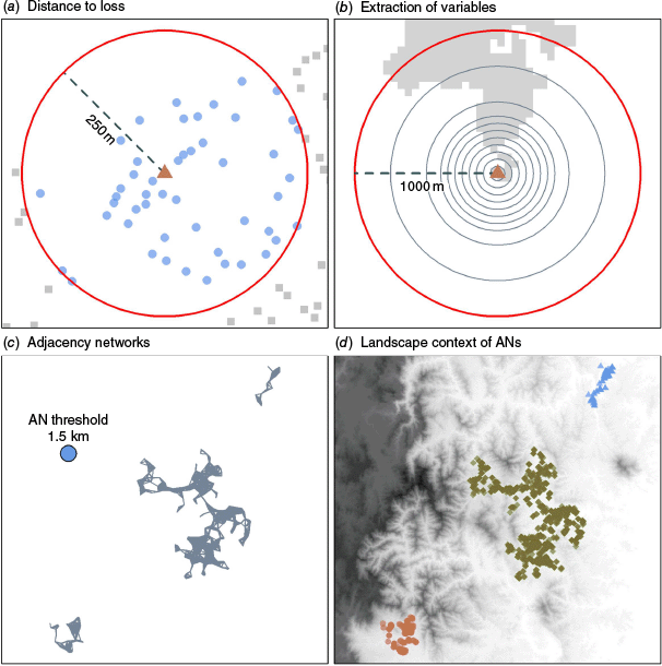
Structures were then clustered into 1.5 km adjacency networks (ANs; 809 total) prior to analysis (Fig. 1c), where an individual network comprised structures within 1.5 km from one another, and any structure more than 1.5 km from the network was deemed to be in a separate network. Spatially grouping structures allowed for control of spatial autocorrelation effects in subsequent analyses. These effects include individual fires, suppression responses across different parts of the landscape and other spatially correlated features not captured by the predictor variables (Fig. 1c, d). The 1.5 km distance threshold was selected based on the spatial distribution of losses, ensuring it was neither too small (e.g. 200 m), which would result in overly fine groupings of structures, nor too large (e.g. 20 km), which could merge different fires into a single AN grouping.
Spatial predictors were extracted for each structure (both loss and non-loss cases), including the numbers of adjacent structures, proportion of cleared land, median canopy height (hereafter canopy height) and terrain ruggedness index (TRI). Data sources are shown in Table 1. Cleared land was defined based on AFDRS fuel grid classifications (urban, non-combustible, built-up, rural, pasture, grass, horticulture or crops) and converted to a binary format (1 = cleared, 0 = vegetated). Other predictors (distance to nearest vegetation, vegetation type, time since fire, etc., further details can be found in Supplementary Material S1) were initially tested but not included in the final modelling as they did not improve predictive performance. Structure counts, cleared land proportion and median canopy height were extracted within a radius of 50, 100, 150, 200, 250, 300, 400, 500, 750, and 1000 m of the structure coordinates (Fig. 1b) following the approach of Price and Bradstock (2013). TRI was also extracted for each point using the method of Wilson et al. (2007) to determine cell-wise TRI values using the eight adjoining grid cells.
| Citation | Data | Extracted predictor | Predictor name | |
|---|---|---|---|---|
| Microsoft building footprints | Centroids of structures | Counts of structures within a given radius. | struc250m | |
| struc750m | ||||
| Matthews et al. (2019) | 50 m grid fuel layer | Proportion of cleared land within a given radius. Area-weighted by intersection with the radius. | clear100m | |
| clear400m | ||||
| Gallant et al. (2009) | ~90 m grid elevation data | Terrain ruggedness index (TRI): the summed absolute difference in elevation between the cell of interest and the immediately adjacent cells. | TRI | |
| Scarth et al. (2019), Scarth et al. (2023) | 95% canopy interception height | Median canopy height (in m) within a given radius. N.B. data source gives height in decimetres. | canheight50 | |
| canheight400 |
Predictor names used in the model equations are also shown.
Extraction of predictors at increasing distance from structures was used for two reasons: firstly the direction of attack from a fire was unknown and could not be accurately inferred from available data, and secondly this approach allowed us to test for the most informative radius for a given predictor, enabling us to determine the distance from a structure where each predictor has the most influence on structure loss, given the resolution of the available data.
Analyses
A generalised linear mixed model (GLMM) with a binomial error structure and logit link was used, with individual structure loss or non-loss as the response variable. A random effect accounted for the ANs in which structures were grouped (757 levels after removing validation data). For model fitting and testing, a 70/30% split was applied, with 3260 loss and 3591 non-loss cases randomly selected for validation.
For the proportional model dataset, a generalised linear model (GLM) with a binomial error structure and logit link was used. Loss proportions were calculated within 1.5 km ANs, including structures within 250 m of a loss, and predictor medians were computed for each AN. ANs with fewer than 15 structures were excluded to avoid low-granularity observations; of the 640 excluded ANs, 414 contained five or fewer structures. A 70/30% split was applied to the remaining 169 ANs for model fitting and testing, resulting in 50 ANs randomly removed for validation and 119 retained for modelling. The proportional loss models used a weighting equivalent to the number of structures in each AN overall (both loss and non-loss).
To assess explanatory value of the predictors, univariate models were fitted using predictors extracted at increasing radii, with Bayesian Information Criterion (BIC; Schwarz 1978) used as metric for both the binomial and proportional models. Multivariate models incorporating all predictors were then fitted, selecting terms at their most informative radii based on univariate analysis, in addition to TRI. The final models were evaluated using true positive (TPR) and true negative rates (TNR) for the binomial model, and r2, mean absolute error (MAE) and bias for the proportional loss model. Predictive accuracy metrics were compared between modelled and validation datasets.
Transformations for predictor data were selected based on lower BIC values found during the univariate analysis: structure counts were ln-transformed, cleared land proportion logit-transformed, and TRI sqrt-transformed, while canopy height remained untransformed. Information on the distributions of predictors in the fitted and validation datasets are provided in Supplementary Material S2. These appendices aggregate the predictions of the models to the AFDRS and provide further information on the models’ performance when used as a spatial output.
Details of the two model’s performance when aggregated to the AFDRS grid are given in Supplementary Material S3. Alternative versions of the models using generalised additive modelling and their predictive performance are shown in Supplementary Material S4. All analyses and plotting were conducted in R (R Core Team 2023), using the terra package (Hijmans 2024) to handle gridded data, sf (Pebesma 2018) for spatial vector data, lme4 (Bates et al. 2015) to fit the generalised linear mixed models, igraph (Csárdi et al. 2024) to define the ANs, mgcv (Wood 2004) to fit generalised additive models and concaveman (Gombin et al. 2020) to define the concave hull of losses to generate predictions within.
Results
In determination of the most appropriate buffer distance, univariate models comparing the buffers from 0 to 1000 m showed the lowest BIC for the 250 and 750 m radius buffer for structure counts (Fig. 2a, c) for the binomial and proportional models respectively (the lower BIC, the greater explanatory value). Odds ratios showed higher structure counts were associated with lower probability of loss/lower proportion of loss (Fig. 2b, d, odds ratios <1). Cleared land at 400 m (binomial model) and 100 m (proportional model) were most informative (Fig. 2e, g), with greater proportions of cleared land related to lower probability/proportion of loss (Fig. 2f, h). Canopy height at the 400 m radii (binomial model; Fig. 2i) and 50 m radii (proportional model; Fig. 2k) returned the lowest BIC. Taller canopy height was associated with increased probability of loss/proportional loss (Fig. 2j, l). Equations for the multivariate models built with these predictors and the inclusion of TRI are shown below:
binlp (binomial) and proplp (proportional) can then be transformed to an estimate of structure loss probability or proportional loss using:
where:
lp = the linear predictor binlp or proplp
struc250m = structure count within 250 m of a structure
struc750m = structure count within 750 m of a structure
clear100m = proportion cleared land within 100 m of a structure
clear400m = proportion cleared land within 400 m of a structure
canheight50 = canopy height within 50 m of a structure (m)
canheight400 = canopy height within 400 m of a structure (m)
TRI = terrain ruggedness index
Plots of the ΔBayesian Information Criterion (BIC) (relative to the most informative BIC) of the univariate models fitted to each buffered value (left side, plots a, c, e, g, i, and k) and odds ratios (right side, plots b, d, f, h, j, l), for structure counts (1st and 2nd rows; ln transformed), cleared land proportion (3rd and 4th rows; logit transformed), and canopy height (5th and 6th rows; ln transformed). The 1st, 3rd and 5th rows show results from the binomial model, and the remainder the proportional model. In all plots, the lowest (best) ΔBIC predictor is indicated by a red rhombus point, with blue circles used elsewhere.
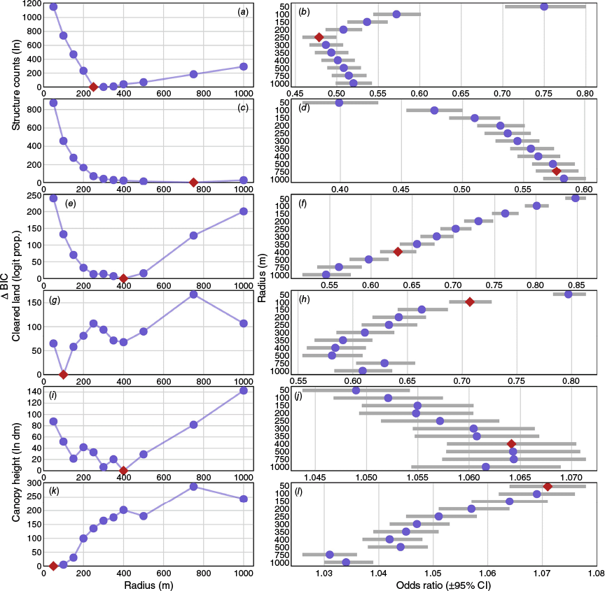
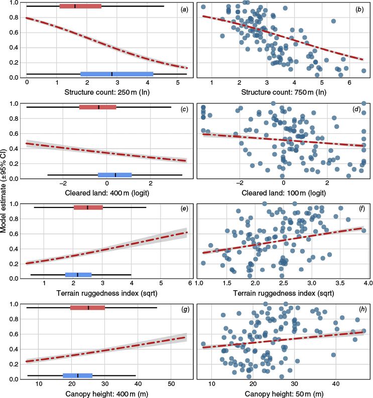
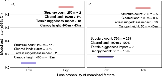
In both models the effects of the shared predictors showed similar relationships. Structure count was the most explanatory predictor in both the binomial and proportional models, as indicated by the largest BIC increase upon removal (Table 2), followed by TRI, canopy height and proportion of cleared land in decreasing importance. Higher structure counts were significantly associated with lower probability of loss at an individual structure level (Fig. 3a), and lower proportional loss (Fig. 3b). Greater cleared land proportions (Fig. 3c, d) and flatter terrain (Fig. 3e, f) were significantly related to lower probability of loss and proportions of loss. Taller canopy height was significantly associated with greater probability of loss in both models (Fig. 3g, h). Full model test statistics and term significance are shown in Table 3. Comparing a structure with predictors indicative of high loss likelihood to one with low likelihood (Fig. 4a) yielded model estimates of 0.91 and 0.07, respectively. For proportional loss, estimates were of similar magnitude with 0.89 for a high-risk area and 0.16 for a lower-risk area (Fig. 4b).
| Terms | Δ BIC binomial | Δ BIC proportional | |
|---|---|---|---|
| Structure count | 670.8 | 679.4 | |
| Terrain ruggedness index | 78.2 | 122.4 | |
| Canopy height | 63.9 | 25.4 | |
| Cleared land | 78.2 | 21.1 |
Model estimated effects (holding other predictors at their means) are shown for structure count (top row, a and b), cleared land proportion (second row, c and d), slope (third row, e and f) and canopy height (fourth row, g and h). Binomial model estimates are shown at left and proportional loss estimates at right. In the binomial model plots, boxplots indicate the data distributions for losses (red shaded) and non-losses (blue shaded). In the proportional model plots, the observations are shown as points. Grey shaded areas on the model estimates are the 95% CI.
| Model | Term | χ2, DF = 1 | P | |
|---|---|---|---|---|
| Binomial | Structure count: 250 m (ln) | 667.137 | <0.0001 | |
| Cleared land: 400 m (logit) | 47.473 | <0.0001 | ||
| Canopy height: 400 m | 71.848 | <0.0001 | ||
| Terrain ruggedness index (TRI) (sqrt) | 87.212 | <0.0001 | ||
| Proportional | Structure count: 750 m (ln) | 684.156 | <0.0001 | |
| Cleared land: 100 m (logit) | 25.928 | <0.0001 | ||
| Canopy height: 50 m | 30.133 | <0.0001 | ||
| TRI (sqrt) | 127.173 | <0.0001 |
Comparison of low and high loss likelihood combinations of predictors variables for the binomial (a) and proportional model (b) as an illustrative example of the combined effects of the model predictors. The predictor values used are shown on the plots below or above the model estimates. Where there was a positive relationship between loss and a given predictor, the 95th percentile value from the dataset was used for the high-loss likelihood estimate and the 5th percentile for the low loss likelihood estimate. Where the relationship between loss and a predictor was negative this process was inverted.
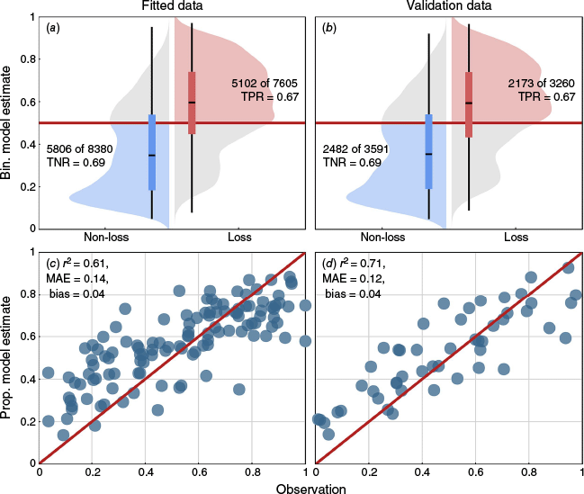
Predictive accuracy for the binomial model was consistent between the fitted (Fig. 5a) and validation datasets (Fig. 5b), with both achieving a TPR of 0.67 and a TNR of 0.69. For both datasets, the median predictions showed reasonable separation between loss and non-loss cases, meaning the model was able to distinguish between the two on average. For the proportional model, r2 was higher for the validation dataset (0.61 vs 0.71; Fig. 5d), compared to the modelled data (Fig. 5c), MAE was similar between datasets (0.14 fitted vs 0.12 validation) and bias remained unchanged (0.04).
Boxplot and density distributions of the binomial (Bin.) model predictions for the fitted data (a), and the validation data (b) disregarding information in the random effect grouping factor in both cases. In (a) and (b) counts of correctly predicted losses (red shaded) and non-losses (blue shaded) are shown with true positive rate (TPR) and true negative rate (TNR) proportions. Predictions for the proportional (Prop.) model on the fitted data are shown in (c), and for the validation data in (d). In (c) and (d), r2, MAE and bias (prediction – observation).
The mapped model outputs show high median loss estimates (Fig. 6c; aggregated predictions for all structures in each grid cell) in areas with structures located within mapped fuel (Fig. 6a, b), highlighting the effect of cleared land on reducing the probability of structure loss. Maximum loss estimates were sensitive to structure count (Fig. 6d), returning lower estimates in areas with more structures. Proportional loss estimates (Fig. 6e; predictions made using cell median values for predictors) gave visually similar results to the median loss estimates (Fig. 6c).
Maps showing the Australian Fire Danger Rating System (AFDRS) fuel types (a), counts of structures (b), the median (c) and maximum (d) model loss estimates for these structures, and the proportional loss estimate model predictions (e). A key for (a) is shown above (a) with white corresponding to land outside the defined fuel types shown in the key, and colour scales for (b) to (e) shown to the right of each plot indicate values.
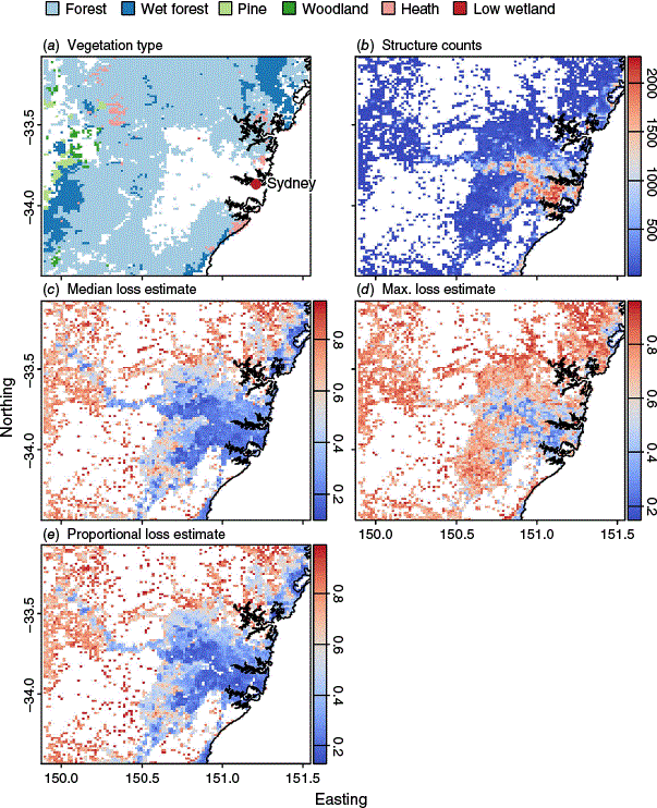
Overall, both the binomial and proportional models showed good performance in predicting structure loss at the individual level (binomial model) and the proportions of structures lost at larger spatial scales. Model predictions made on the AFDRS grid show clear spatial patterns in the estimates of structure loss, with the binomial model offering different methods to aggregate the predictions to grid scale (median and maximum probability; Fig. 6).
Discussion
The models described here are designed to predict the factors which may predispose structures to loss during fire. With this aim we focussed on the influence of landscape factors and structure counts as descriptors of structure loss. Both models retained terms for structure count (within 250 and 750 m for the binomial and proportional model respectively), cleared land within 400 and 100 m, canopy height within 400 and 50 m and TRI. Taken together, these indicate lower probability of structure loss where land (a) is 100% cleared surrounding the structure in a buffer (defensible space), (b) has shorter canopy height in surrounding vegetation, (c) is on flat ground, and (d) has a higher number of structures nearby. These results are in concordance with other studies which found defensible space (Syphard et al. 2014), TRI (Price and Bradstock 2013) and surrounding structure density (Syphard et al. 2012) which are important predictors of structure loss. Notably, this study found a larger defensible space was required (buffer distance between the structure and adjacent fuel) – 400 m for the binomial model and 100 m for the proportional model – compared to previous studies. In contrast, Gibbons et al. (2012) and Syphard et al. (2014) reported 40 m, and up to 30 m, respectively. This difference is likely due to the use of relatively low-resolution spatial data used in this study to characterise surrounding land compared to the previous research. Studies which directly measure these properties with respect to the direction of fire attack will give a more accurate estimate for the buffer sizes of defensible space. In this study, buffer sizes are likely influenced by data resolution, capturing vegetation surrounding a structure rather than only in the direction the fire travelled before causing its loss. The 1-km proportion of forested land identified by Price and Bradstock (2013) as a predictor of house loss, was calculated similarly to the cleared land in this study, suggesting that this difference in methodology may account for the variation between studies.
The binomial model showed reasonable classification accuracy (TPR = 0.67 and TNR = 0.69 on the validation data; Fig. 5). The proportional loss model also showed a good predictive fit (r2 = 0.71 on the validation data and 0.61 on the calibration/fitting data).
Other regression model-based studies have identified different primary contributors to their predictions. For example, Wilson and Ferguson (1986) and Blanchi et al. (2010) used the Forest Fire Danger Index (FFDI) to infer house loss, while Gibbons et al. (2012) focussed on fuels and their attributes (cover within 40 m of houses, fuel type, upwind distance to fuels and fuel treatment). Harris et al. (2012) found that adjusted fire danger indices and fire relative energy were the best predictors of house loss, and Duff et al. (2019) incorporated convection, ember density and flame height as the sole contributors to their regression-based house loss model, while Duff and Penman (2021) added perceived slope, presence of fuels within 40 m and percentage of fuel within 100 m as predictors of loss.
Predictors of house loss can be broadly classified into weather-, fire behaviour-, or fuels-based factors. In the model presented here, we used fuels-based, topographic (TRI) risk factors, and structure counts to predict structure loss. This approach has allowed the development of a model which aligns well with the AFDRS operational framework and can be interpreted alongside AFDRS forecasts, e.g. the FBI. To ensure compatibility with existing AFDRS models and data, the impact forecasts generated in this study are aggregated to the AFDRS 1.5 × 1.5 km grid (Fig. 6).
Using models based on observed data
Regression models have been widely used for predicting structure loss due to their simplicity in construction and interpretation. More complex models with a larger number of input variables and interactions may or may not provide more accurate predictions. For example, Duff et al. (2019) showed a machine learning approach yielded a weighted accuracy of 92% with significant contributions from the predictor variables convection, wind speed, ember density, flame height and several derived variables. However, the use of increasingly complex models runs the risk of overfitting, where the model performs well on the test dataset, but lacks generalisability to other data, particularly the spatial data which will necessarily underlie predictions made at national scale. Difficulties in adapting the output for expression at grid scale, rather than for individual house level used by many of these models, renders them less suitable for use in operations and within the context of the AFDRS. Given that outputs in the AFDRS framework are updated multiple times throughout the day, recalculating outputs at the national scale using models which rely on predictions at structure level (m’s), would impose significant computational resources and would likely require data resolution higher than what is currently available at the national scale.
The variety of input variables used by different house loss models indicates the important role that data plays in the model development process. Individual models are (necessarily) selected on their ability to accurately explain the data they use in their construction. To overcome this selectivity issue and generate more universal and robust structure loss models, the development of more complex models will accordingly require large datasets. Collection of a wider range of data, e.g. fire direction, the distance to vegetation at the angle of fire attack, suppression effort and structural characteristics of the buildings, would provide useful data for different types and scales of modelling approaches.
Potential improvements
Fuels, their proximity to structures, weather affecting a structure, structure design (i.e. built before implementation of current standards in building design in fire-prone areas), proximity to other structures, ember release, flame intensity and radiant output reaching a structure are all important factors contributing to structure loss. As the AFDRS is national in scope, we sought to forecast structure loss across all the different fuels present, and the vegetation maps used partly satisfied this requirement. The model described here will be trialled within southeastern Australia and tested or refit once more data becomes available from other Australian fire agencies. While the AFDRS is constrained to weather inputs at a 1.5 × 1.5 km resolution, the advent of a combined national fuel map at finer scales (e.g. 10s of metres) will aid calculations of likely structure loss at the level of individual structures. We have shown that this approach can be aggregated up to the AFDRS grid scale and provide a more nuanced output.
In their current form the impact models estimate the probability of complete destruction of a structure (or the proportion of structures) assuming a fire occurs in the grid cell of interest and reaches the structure of interest (or as close to it as possible considering fuel clearances around the structure). The models are static in that they are weather agnostic and only use fuel proximity, slope, canopy height and structure count as input variables. Future work may provide refinements to the current model (with higher resolution fuel layers and further data of structure losses), and enable the generation of a metric describing structure loss that incorporates fire management agency feedback after review of the prototype spatial layers. Future model improvement may also consider using the predominant AFDRS fuel type as one of the predictors, however this approach is contingent on there being sufficient structure loss data available for each fuel.
The impact model and the AFDRS
The AFDRS FBI describes the general behaviour of a fire (rate of spread, intensity, flame height, spotting distance), however, it does not describe the likelihood of impact on structures within a grid cell. The impact model focusses on structure loss as a proxy for loss of life (which may be less likely in built-up non-residential areas, e.g. warehousing or manufacturing areas); future versions could include vulnerability, and a range of other assets including cultural and environmental assets. In its current form the impact model aims to inform fire and land management agencies of the probability of a fire impacting on structures in a grid cell, were a fire to spread there and can be interpreted in concert with the prevailing FBI. Through this method, cells with high estimates of potential impact and predicted high fire danger at a given time can be more easily identified.
Decisions arising from impact index predictions interpreted alongside the FBI (predicted fire severity), ignition likelihood (e.g. Penman et al. 2013), the locations of current wildfires and the likelihood of their spread to surrounding grid cells could include initiating evacuations early, or prepositioning suppression resources at strategic locations prior to a day of the dangerous fire potential. The impact index can be used alongside products within the AFDRS suite, such as FBI, to complement decision-making.
Conclusion
The impact index aims to provide decision makers with an objective likelihood forecast that will provide output in a format consistent with other AFDRS products (e.g. FBI), with which it can be combined into a fire behaviour weighted output and is designed for use by decision makers and Fire Behaviour Analysts. In an Incident Management Team, objective metrics provide valuable intelligence that can be used to temper more subjective assessments of what is likely to happen during a running fire. While an index can only provide an estimate (with inherent uncertainty), the introduction of the impact index will make a significant contribution to tools available to those making important decisions regarding wildfire control in Australia. This model is a first step in providing this information and will be refined or replaced as understanding of the drivers of structure loss during wildfire progresses.
Data availability
The data that support this study cannot be publicly shared due to ethical or privacy reasons and may be shared upon reasonable request to the corresponding author if appropriate.
Declaration of funding
The authors acknowledge the financial support of the Minderoo Foundation, Australian and New Zealand National Council for fire and emergency services (AFAC) through the National Aerial Firefighting Centre (NAFC) Resource to Risk project, fire agencies from all jurisdictions in Australia, and the Commonwealth. No specific grant numbers were associated with this funding. The funding organisations played no role in preparation of this work, or in the decision to submit it for publication.
Acknowledgements
The authors would like to acknowledge valuable feedback and comments from individuals in fire and land management agencies in Australia. We acknowledge fruitful discussions with Dr Musa Kilinc, whose original house loss model formed the basis of this work, Drs Owen Price and Michael Bedward, for analytic inspiration, and Dr Billy Tan and Hannah Kranz for reviewing a draft of this publication. We also thank two anonymous reviewers whose comments substantially improved this paper.
References
Ager AA, Day MA, Alcasena FJ, Evers CR, Short KC, Grenfell I (2021) Predicting Paradise: modeling future wildfire disasters in the western US. Science of The Total Environment 784, 147057.
| Crossref | Google Scholar | PubMed |
Bates D, Maechler M, Bolker B, Walker S (2015) Fitting linear mixed-effects models using lme4. Journal of Statistical Software 67(1), 1-48.
| Crossref | Google Scholar |
Blanchi RM, Leonard JE, Leicester RH (2006) Bushfire Risk at the Rural/Urban Interface. In ‘Australasian Bushfire Conference’. pp. 6–9. Available at https://www.fireandbiodiversity.org.au/images/publications/conference-2006/Bushfire_risk_at_the_rural-urban_interface.pdf
Blanchi R, Lucas C, Leonard J, Finkele K (2010) Meteorological conditions and wildfire-related house loss in Australia. International Journal of Wildland Fire 19, 914-926.
| Crossref | Google Scholar |
Blanchi R, Leonard J, Haynes K, Opie K, James M, de Oliveira FD (2014) Environmental circumstances surrounding bushfire fatalities in Australia 1901–2011. Environmental Science & Policy 37, 192-203.
| Google Scholar |
Collins KM, Penman TD, Price OF (2016) Some wildfire ignition causes pose more risk of destroying houses than others. PLoS One 11, e0162083.
| Crossref | Google Scholar |
Csárdi G, Nepusz T, Traag V, Horvát Sz, Zanini F, Noom D, Müller K (2024) igraph: Network Analysis and Visualization in R. 10.5281/zenodo
Duff TJ, Penman TD (2021) Determining the likelihood of asset destruction during wildfires: modelling house destruction with fire simulator outputs and local-scale landscape properties. Safety Science 139, 105196.
| Crossref | Google Scholar |
Gibbons P, Van Bommel L, Gill AM, Cary GJ, Driscoll DA, Bradstock RA, Knight E, Moritz MA, Stephens SL, Lindenmayer DB (2012) Land management practices associated with house loss in wildfires. PLoS One 7, e29212.
| Crossref | Google Scholar | PubMed |
Gibbons P, Gill AM, Shore N, Moritz MA, Dovers S, Cary GJ (2018) Options for reducing house-losses during wildfires without clearing trees and shrubs. Landscape and Urban Planning 174, 10-17.
| Crossref | Google Scholar |
Gombin J, Vaidyanathan R, Agafonkin V (2020) concaveman: A Very Fast 2D Concave Hull Algorithm (R package version 1.1.0). Available at https://CRAN.R-project.org/package=concaveman
Harris S, Anderson W, Kilinc M, Fogarty L (2012) The relationship between fire behaviour measures and community loss: an exploratory analysis for developing a bushfire severity scale. Natural Hazards 63, 391-415.
| Crossref | Google Scholar |
Haynes K, Handmer J, Mcaneney J, Tibbits A, Coates L (2010) Australian bushfire fatalities 1900–2008: exploring trends in relation to the ‘Prepare, stay and defend or leave early’ policy. Environmental Science & Policy 13, 185-194.
| Crossref | Google Scholar |
Hollis JJ, Matthews S, Fox-Hughes P, Grootemaat S, Heemstra S, Kenny BJ, Sauvage S (2024) Introduction to the Australian Fire Danger Rating System. International Journal of Wildland Fire 33, WF23140.
| Crossref | Google Scholar |
Hijmans R (2024) terra: Spatial Data Analysis. R package version 1.7-71. Available at https://CRAN.R-project.org/package=terra
Kenny BJ, Matthews S, Sauvage S, Grootemaat S, Hollis JJ, Fox-Hughes P (2024) Australian Fire Danger Rating System: implementing fire behaviour calculations to forecast fire danger in a research prototype. International Journal of Wildland Fire 33(4), WF23142.
| Crossref | Google Scholar |
Leonard J, Blanchi R (2005) Investigation of bushfire attack mechanisms involved in house loss in the ACT Bushfire 2003. Bushfire CRC report. Available at https://www.naturalhazards.com.au/crc-collection/downloads/act_bushfire_crc_report.pdf
Massada AB, Radeloff VC, Stewart SI, Hawbaker TJ (2009) Wildfire risk in the wildland–urban interface: a simulation study in northwestern Wisconsin. Forest Ecology and Management 258(9), 1990-1999.
| Crossref | Google Scholar |
Nolan RH, Anderson LO, Poulter B, Varner JM (2022) Increasing threat of wildfires: the year 2020 in perspective: A Global Ecology and Biogeography special issue. Global Ecology and Biogeography 31, 1898-1905.
| Crossref | Google Scholar |
Peace M, McCaw L (2024) Future fire events are likely to be worse than climate projections indicate – these are some of the reasons why. International Journal of Wildland Fire 33(7),.
| Crossref | Google Scholar |
Pebesma E (2018) Simple features for R: standardized support for spatial vector data. The R Journal 10(1), 439-446.
| Crossref | Google Scholar |
Penman TD, Bradstock RA, Price O (2013) Modelling the determinants of ignition in the Sydney Basin, Australia: implications for future management. International Journal of Wildland Fire 22, 469-478.
| Crossref | Google Scholar |
Penman SH, Price OF, Penman TD, Bradstock RA (2019) The role of defensible space on the likelihood of house impact from wildfires in forested landscapes of southeastern Australia. International Journal of Wildland Fire 28, 4-14.
| Crossref | Google Scholar |
Price O, Bradstock R (2013) Landscape scale influences of forest area and housing density on house loss in the 2009 Victorian bushfires. PLoS One 8, e73421.
| Crossref | Google Scholar | PubMed |
Price OF, Whittaker J, Gibbons P, Bradstock R (2021) Comprehensive Examination of the determinants of damage to houses in two wildfires in eastern Australia in 2013. Fire 4(3), 44.
| Crossref | Google Scholar |
Ramsay GC, Mcarthur NA, Dowling VP (1987) Preliminary results from an examination of house survival in the 16 February 1983 bushfires in Australia. Fire and Materials 11, 49-51.
| Crossref | Google Scholar |
Raveendran N, Zhu H, Li H, Sofronov G (2024) Wildfire loss modeling: a flexible semiparametric approach. North American Actuarial Journal 29, 329-344.
| Crossref | Google Scholar |
R Core Team (2023) ‘R: A Language and Environment for Statistical Computing.’ (R Foundation for Statistical Computing: Vienna, Austria) Available at https://www.R-project.org/
Scarth P, Armston J, Lucas R, Bunting P (2019) A structural classification of Australian vegetation using ICESat/GLAS, ALOS PALSAR, and Landsat sensor data. Remote Sensing 11(2), 147.
| Crossref | Google Scholar |
Scarth P, Armston J, Lucas R, Bunting P (2023) Vegetation Height and Structure - Derived from ALOS-1 PALSAR, Landsat and ICESat/GLAS, Australia Coverage. (Version 1.0) [Dataset] Terrestrial Ecosystem Research Network. Available at https://portal.tern.org.au/metadata/TERN/de1c2fef-b129-485e-9042-8b22ee616e66
Schwarz GE (1978) Estimating the dimension of a model. Annals of Statistics 6(2), 461-464.
| Crossref | Google Scholar |
Strahan K (2020) An archetypal perspective on householders who ‘wait and see’ during a bushfire. Progress in Disaster Science 7, 100-107.
| Crossref | Google Scholar |
Syphard AD, Keeley JE, Massada AB, Brennan TJ, Radeloff VC (2012) Housing arrangement and location determine the likelihood of housing loss due to wildfire. PLoS One 7(3), e33954.
| Crossref | Google Scholar | PubMed |
Syphard AD, Brennan TJ, Keeley JE (2014) The role of defensible space for residential structure protection during wildfires. International Journal of Wildland Fire 23, 1165-1175.
| Crossref | Google Scholar |
Tedim F, Leone V, Amraoui M, Bouillon C, Coughlan MR, Delogu GM, Fernandes PM, Ferreira C, McCaffrey S, McGee TK (2018) Defining extreme wildfire events: difficulties, challenges, and impacts. Fire 1, 9.
| Crossref | Google Scholar |
Tolhurst KG, Shields B, Chong DM (2008) Phoenix: development and application of a bushfire risk management tool. Australian Journal of Emergency Management 23, 47-54.
| Google Scholar |
Whittaker J, Clark A (2021) Research to improve community warnings for bushfire. The Australian Journal of Emergency Management 36, 13-14.
| Google Scholar |
Whittaker J, Taylor M, Bearman C (2020) Why don’t bushfire warnings work as intended? Responses to official warnings during bushfires in New South Wales, Australia. International Journal of Disaster Risk Reduction 45, 101476.
| Crossref | Google Scholar |
Wilson AA, Ferguson IS (1986) Predicting the probability of house survival during bushfires. Journal of Environmental Management 23, 259-70.
| Google Scholar |
Wilson MFJ, O’Connell B, Brown C, Guinan JC, Grehan AJ (2007) Multiscale terrain analysis of multibeam bathymetry data for habitat mapping on the continental slope. Marine Geodesy 30(1–2), 3-35.
| Crossref | Google Scholar |
Wood SN (2004) Stable and efficient multiple smoothing parameter estimation for generalized additive models. Journal of the American Statistical Association 99, 673-686.
| Crossref | Google Scholar |