

Different approaches make comparing studies of burn severity challenging: a review of methods used to link remotely sensed data with the Composite Burn Index
Colton W. Miller A B * , Brian J. Harvey A , Van R. Kane A , L. Monika Moskal A and Ernesto Alvarado A
A School of Environmental and Forest Sciences, College of the Environment, University of Washington, Box 352100, Seattle, WA 98195, USA.
B Present address: Vibrant Planet, PBC, Pioneer Commerce Center 11025 Pioneer Trail, Suite 200a, Truckee, CA 96161, USA.
International Journal of Wildland Fire 32(4) 449-475 https://doi.org/10.1071/WF22050
Submitted: 11 April 2022 Accepted: 23 December 2022 Published: 7 February 2023
© 2023 The Author(s) (or their employer(s)). Published by CSIRO Publishing on behalf of IAWF. This is an open access article distributed under the Creative Commons Attribution 4.0 International License (CC BY).
Abstract
The Composite Burn Index (CBI) is commonly linked to remotely sensed data to understand spatial and temporal patterns of burn severity. However, a comprehensive understanding of the tradeoffs between different methods used to model CBI with remotely sensed data is lacking. To help understand the current state of the science, provide a blueprint towards conducting broad-scale meta-analyses, and identify key decision points and potential rationale, we conducted a review of studies that linked remotely sensed data to continuous estimates of burn severity measured with the CBI and related methods. We provide a roadmap of the different methodologies applied and examine potential rationales used to justify them. Our findings largely reflect methods applied in North America – particularly in the western USA – due to the high number of studies in that region. We find the use of different methods across studies introduces variations that make it difficult to compare outcomes. Additionally, the existing suite of comparative studies focuses on one or few of many possible sources of uncertainty. Thus, compounding error and propagation throughout the many decisions made during analysis is not well understood. Finally, we suggest a broad set of methodological information and key rationales for decision-making that could facilitate future reviews.
Keywords: burn severity, CBI, Composite Burn Index, dNBR, dNDVI, fire severity, GeoCBI, landsat imagery, NBR, NDVI, RdNBR, remote sensing, spectral index.
Introduction
Estimates of burn severity, here defined as the ecological effects of fire, or fire-caused change (Lentile et al. 2006), inform immediate post-fire recovery projects, future fuel treatments, and long-term ecosystem analysis (Miller and Thode 2007). In the immediate post-fire environment, common priorities are to preserve the soil and maintain the vegetation community (Fernández-García et al. 2018a). A second key function of severity assessments is to understand how fire effects vary with ecosystem composition and structure. Linking pre-fire conditions with potential post-fire outcomes helps managers to design better fuel treatments, such as thinning and prescribed fires (Churchill et al. 2013, 2022; Larson et al. 2022). Severity estimates can also help to predict long-term consequences to a post-fire ecosystem (Macdonald 2007), such as changes to forest succession (Johnstone and Chapin 2006). Managers need predictive models of wildland fire effects on vegetation communities, wildlife populations, and hydrologic function (Sorbel and Allen 2005), and ongoing records of fire effects allow ecologists to assess effects of climate change over time.
Commonly measured fire effects on the ground include consumption of vegetation, destruction of leaf chlorophyll, exposed soil, charred stems, and altered moisture (Epting et al. 2005). These ecological impacts lead to spectral, thermal, and structural changes on the land surface, which can be captured by remote sensors (Epting et al. 2005; Mallinis et al. 2018). Combinations of these post-fire soil and vegetation conditions, including those with multiple ecosystem attributes, are used to assess burn severity (Table 1). Methods may be quantitative or qualitative; all incorporate a choice of fire-related variables that depend on management and ecological objectives as well as sampling scale (Key and Benson 2006). Post-fire site characteristics are typically considered relative to the pre-disturbance environment (Miller and Thode 2007), so severity is also a subjective measurement that can change with the time of observation and information available (Lentile et al. 2006).

|
The size and variability of wildland fires pose several challenges for characterising fire effects on the ground (Chen et al. 2011). First, accessing remote locations where fires have occurred requires resource-intensive and logistically challenging fieldwork (Morgan et al. 2014). Second, the heterogeneity in burn severity across burned landscape requires many plots to represent the range of conditions in burned areas (Morgan et al. 2014). Finally, many burned areas are poorly represented spatially from field plots alone, due to the sheer size of burned areas relative to the size and number of field plots that are logistically possible (De Santis and Chuvieco 2007).
Remote sensing is a powerful tool to understand spatial patterns across burned landscapes, providing a synoptic view from space- or airborne sensors, (Lentile et al. 2006; Wulder et al. 2009; Soverel et al. 2010) and allowing observation of post-fire effects inaccessible from the ground (Key and Benson 2006; Lentile et al. 2006; Murphy et al. 2008). That said, although remotely sensed data provide extensive spatial and temporal coverage that field observations lack (Schepers et al. 2014), they must be linked to ‘ground-truth’ field data (Morgan et al. 2014). The choice of field data depends on the goals of the study; there is no one-size-fits-all approach to evaluating severity (Keeley 2009). The range of potential research questions and applications of these assessments requires different approaches determined by a combination of management, ecological goals, and field sampling designs (Ryan and Noste 1985).
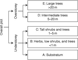
The Composite Burn Index (CBI) integrates multiple metrics across vegetation strata and soil, which, used together (as a measure of site burn severity), provide an overall scope of fire damage (Key and Benson 2006) (Fig. 1). Individual components of the index may also be considered separately, depending on post-fire management needs (Key and Benson 2006; Zhu et al. 2006; Keeley 2009). CBI has been adapted in many ways, including general modifications such as the geometrically structured CBI (GeoCBI, De Santis and Chuvieco 2009), and site-specific modifications such as adding or omitting specific attributes (Epting et al. 2005; Allen and Sorbel 2008; Hoy et al. 2008; Schepers et al. 2014; Fernández-García et al. 2018b).
|
CBI has emerged as a popular measure of field-based severity in remote sensing for several reasons. First, the rapid protocol allows quick deployment and assessment over large landscapes (Parks et al. 2019). Second, CBI has generally robust relationships with field measures (Saberi et al. 2022) and satellite spectral fire severity indices (French et al. 2008), providing strong support for its use to estimate fire effects across landscapes (Parks et al. 2019). Third, for general assessments of severity, the CBI may be more complete than other classification systems based on single indicators of burn severity (Sikkink 2015).
In addition to the CBI, several alternative composite severity measures have been published in the fire ecology literature. The GeoCBI accounts for differences in fractional cover of each stratum and changes in leaf area index (LAI) for the intermediate and tall tree strata (De Santis and Chuvieco 2009). Fractional cover and LAI describe the influence of vegetation cover on reflectance of different strata within a given plot, and from a remote sensing point of view, the spectral response of a plot is strongly related to the vegetation coverage per stratum (De Santis and Chuvieco 2009). Other modified versions of the CBI include a Weighted CBI (WCBI) (Cansler and McKenzie 2012) and a Burn Severity Index (BSI) (Loboda et al. 2013). The WCBI generally uses the original CBI protocol for sampling severity across strata, but it weights scores by the fraction of cover for each stratum. Although the method is similar to the GeoCBI in that regard, specific weights are study dependent. The BSI was introduced by Loboda et al. (2013) as a less rigorous approach that mimics CBI plots but saves time in the field.
Many field measures of severity were designed to scale across broad landscapes using remotely sensed data, based on the underlying ecological causes that drive changes in spectral reflectance between pre- and post-fire landscapes (Supplementary Table S1). The ecosystem attributes characterised by the CBI and related composite severity measures span the range of change expected to be captured by remotely sensed data. Overall, studies that use remotely sensed data to link to continuous field measures based on composite severity measures follow a similar methodological framework to each other (Fig. 2). However, a number of key decisions are made at each step. Differences in these decisions result in studies that use many unique avenues, and we have limited understanding on how that may affect findings across studies. The range of choices available for analysis at each step may, in totality, be considered a ‘decision menu’ that depends on the research questions and preferred methodological approaches of the study author(s).

|
To our knowledge, no study has yet summarised the methods and important decision points that link remotely sensed data to CBI as a continuous measure. However, studies such as Stambaugh et al. (2015) demonstrate the potential for methodological decisions to strongly influence the relationships between remotely sensed data and field observations. For example, R2 values for the same set of plots ranged from 0.18 to 0.78 depending on whether models used remotely sensed data from initial versus extended assessments, were processed with interpolation or not, and whether they used the delta normalised burn ratio (dNBR) or relativised dNBR (RdNBR). This example highlights the difficulty of comparing model results across studies where methodologies may differ. However, the existing body of literature linking CBI measures to remotely sensed data lacks a comprehensive review of the possible methodological choices that can be made during analysis. This paper sought to conduct a review of the many choices of the ‘decision menu’ and identify the limitations imposed by the lack of consensus in modelling approaches.
The goal of this review was to compare empirical methods used to estimate burn severity measured with CBI both in the field and through remote sensing to understand the impacts of key analytical decisions and research gaps in the existing literature. We did this by exploring:
Where and when have studies been conducted?
How is burn severity measured in the field?
How is burn severity measured from satellites?
How are field observations and remotely sensed data modelled together?
Addressing these key questions from our review of 62 studies will improve our understanding of the state of the science regarding sampling of post-fire environments and the ability to map burned landscapes using remotely sensed data. Additionally, the aggregation of research results from the numerous studies that used a variety of analytical methods will provide insights into whether findings may be generalised across studies or are too study specific to interpret in such a manner.
Methods
Review framework
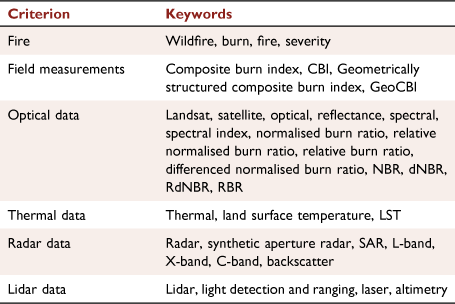
We developed a procedure to guide our process for conducting a systematic literature search, identifying relevant articles, and extracting data for analysis. This review broadly follows the framework developed by Pullin and Stewart (2006) for conducting systematic reviews in conservation and environmental management. Their guidelines for conducting systematic reviews are based on evaluating the effectiveness of management and policy interventions, but we only used their approach to develop a search protocol and to identify and review relevant studies to generate a database from papers that used remotely sensed data and continuous measures of burn severity based on the CBI. Therefore, our work does not investigate the efficacy of a specific treatment (e.g. mechanical thinning or prescribed fire) as the systematic review protocol dictates. Our search criteria were based on fire and field measurements and four remote sensing technologies (optical, thermal, radar, and lidar) (Table 2). For each criterion, a set of keywords was developed for the database queries (see next section).
|
Database queries
The CAB Direct (https://www.cabdirect.org), Environmental Science Collection (https://proquest.libguides.com/environmentalsciencecollection), and Web of Science (https://www.webofknowledge.com) databases were systematically searched for original research that investigated the relationships between remotely sensed data and continuous measures of burn severity assessed with the CBI or GeoCBI. Search terms were combined through Boolean operators so that each query contained the keywords for fire, field measurements, and one remote sensing technology. We used the resulting expression to search abstracts in each database. After combining the results from all three databases, duplicate entries were removed (Supplementary Fig. S1). Any studies that we missed would mainly have been studies published in a journal outside of our database queries (CAB Direct, Environmental Science Collection, Web of Science) or not having the keywords in our search.
Screening and data extraction
Articles were screened to determine whether each entry met the inclusion criteria. Articles were excluded if they (1) did not use CBI/GeoCBI measurements, (2) used simulated CBI/GeoCBI or simulated remotely sensed data, (3) did not analyse CBI/GeoCBI measurements as continuous variables, or (4) were not in English. We focused on the use of CBI as a continuous variable because it provides a more flexible approach than categorical measures that classify measurements into bins such as low, moderate, and high severity. Continuous data can be adapted to multiple different ecological phenomena. For example, different studies may use various threshold breakpoints for different levels of severity depending on the model used and the user’s needs (Boucher et al. 2017), or chosen according to the relevant ecological effects (Hall et al. 2008; Cansler and McKenzie 2012). However, severity values are frequently classified in order to compare multiple fires, analyse spatial patterns, or communicate with managers regarding prioritisation of response (Cansler and McKenzie 2012). Readers may find additional insights into the use of categorical observations of severity in Cansler and McKenzie (2012).
We selected all empirical studies published in peer-reviewed scientific journals through 2019, excluding published literature reviews, dissertations and theses, and government reports. All articles matching the review criteria were retained regardless of the study’s location or ecosystem type. Four additional articles were found through searching the literature cited of the papers included in our search. The articles that met our inclusion criteria were reviewed to extract the relevant information, which was entered in a rubric format. The data for each paper were captured in individual databases for information at the article level (Supplementary Table S2), fire level (Supplementary Table S3), and comparison level (Supplementary Table S4). We compiled 62 studies based on the structured database queries; a list of studies included in this review and the number of field observations to remotely sensed data comparisons extracted for analysis are included in Supplementary Information S2.
Analysis
To locate fires examined by studies included in this review, we used a combination of georeferenced study maps, the published manuscripts, provided coordinates, or ancillary databases (Sikkink et al. 2013; Picotte et al. 2019; CAL FIRE 2020; MTBS 2021). Fires were mapped for cases where we could confidently identify the study fire based on name, location, size, number of field plots, or other identifying characteristics. The spatial mapping of fires allowed us to overlay terrestrial ecosystems of the world (Olson and Dinerstein 2002) and identify which ecosystems may be more or less understood. For fire size, information was found either in the study itself or through ancillary databases.
Although our focus was on the use of burn severity as a continuous variable, many included studies that used continuous data in their analysis also reported thresholds used for classifying burn severity. In such cases, we recorded the distribution of field plots classified by unburned, low, moderate, or high burn severity. These data were assessed in two ways: (1) by summing the number of plots per severity category across the studies; and (2) calculating the proportion of plots placed into different burn severity classes. By assessing classified data, we were able to present some results on the variability of the threshold values used to bin continuous observations. Additionally, because many studies did not show a distribution of continuous plot severity scores, we used this subset of studies that provided classified distributions to gain some understanding of how plot severity varied across studies.
To assess the timing of field campaigns, we used the date of ignition for the fire and date of field sampling. The smallest temporal grain we could identify for cases was to the nearest month. Results were limited to studies that reported both the timing of fires (or studied fires that where ignition date was available elsewhere) and the timing of field campaigns.
In some cases, we contacted authors to ask for information not provided in published manuscripts such as field plot size and timing, index value extraction methods, etc. All summary statistics and figures – with the exception of the study map – were conducted using the R programming language (R Core Team 2017). Where presented, standard deviations were calculated using the population standard deviation equation (Zar 1999). Due to missing information, some summary statistics and analyses are based only on cases where data were available. The number of studies, fires, or comparisons for each analysis are presented in each relevant table or figure caption or in the figure itself.
Results
Study information
Studies using CBI, interannual trends, and main journals
The systematic search resulted in 62 papers published in 2004–2019. All used field measures of burn severity based on the CBI protocol (CBI, GeoCBI, WCBI, BSI) as a continuous measure to integrate with remotely sensed data. One to nine papers were published each year (μ = 4.1, σ = 2.2; Supplementary Fig. S2a), with no significant linear trend over time (t = 1.422, P = 0.179). The 62 articles were in 17 scientific journals; half (31) were in either Remote Sensing of Environment or International Journal of Wildland Fire (Supplementary Fig. S2b).
Fire data
Location of fires
For the 62 studies, 352 of 401 fires were uniquely identified and geospatially located (Fig. 3a). Study fires were most commonly located in temperate conifer forests (185 fires). Less commonly studied ecosystems included boreal forests/taiga (51), temperate broadleaf and mixed forests (47), deserts and xeric shrublands (38), mediterranean forests, woodlands, and scrubs (19), and tundra (9). One fire was studied in each of the following: flooded grasslands and savannas, temperate grasslands, savannas and shrublands; and tropical and subtropical grasslands, savannas and shrublands. Fires sampled were mostly in the Northern Hemisphere, especially in the United States (283) and Canada (22). Fires were also sampled in China (17), Spain (15), Russia (5), Australia (2), Greece (2), and Belgium, Portugal, and Burkina Faso (1 each). Two fires from Miller et al. (2009) and 36 from Parks et al. (2019) lacked sufficient information to identify the locations of fires. In the United States, fires were mainly in temperate conifer forests, deserts and xeric shrublands in the West.

|
Number of fires per study
Each study reported 1–263 fires (μ = 9.9 ± 4.9; η = 3); 23 investigated a single fire. Of the 62 studies reviewed, only 53 explicitly stated the number of fires in the analysis. The other nine studies either reported multiple or several fires (7), an unknown number (1), or did not specify (1).
Timing and type of fires
The earliest identified fire occurred in 1994 and the latest in 2017 (Fig. 3b); 401 unique fires with known ignition dates were identified. Most fires (194/total) were either explicitly labelled as wildfires or classified as such by Monitoring Trends in Burn Severity, a program that maps burn severity and perimeters for fires over 1000 acres in the western USA, and 500 acres in the eastern USA (Eidenshink et al. 2007). Others were prescribed fires (74), wildland use fires (28), and a combination of prescribed and wildland fires (1). Of the remaining 104 fires, four specified only that they were caused by lightning; the rest (96) did not explicitly identify fire type, but most were likely also wildland fires.
Fire sizes
For the 328 fires where information was available, the range of fire sizes was 28–730 855 ha (μ = 18 005, σ = 58 067; Fig. 3c); the majority (65%) were <5000 ha. The sizes of 74 fires were not explicitly given or found in supplementary searches; sometimes this information was not stated (44), was provided as a sum across several fires (3), or the study reported only the regional burn area and not the specific fire studied (1).
Field data
Types of field data used and variation by year
van Wagtendonk et al. (2004) was the first study to use CBI as a continuous measure of burn severity, following its introduction at a Joint Fire Science Conference and Workshop by Key and Benson (1999) (Fig. 4a). Studies using the GeoCBI as a continuous variable to link to remotely sensed data were first published in 2009 (De Santis and Chuvieco 2009). Most of the studies reviewed relied on these protocols, but four investigated modifications such as weighted versions (WCBI) (Soverel et al. 2010; Cansler and McKenzie 2012; Mallinis et al. 2018) or BSI (Loboda et al. 2013) (Table 3). The GeoCBI, WCBI, and BSI emerged as alternate approaches to field sampling, but CBI remained the most common composite severity measure throughout this review.

|

|
Most (57) studies used a single method (e.g. CBI, GeoCBI, or WCBI) to measure burn severity on the ground; CBI on its own comprised 45 of the 62 papers reviewed in this study, and GeoCBI alone was used in 12 studies (Fig. 4b). Only three papers incorporated multiple methods of measuring severity on the same fire and were compared whether different field methods resulted in better or worse relationships with remotely sensed data (De Santis and Chuvieco 2009; Cansler and McKenzie 2012; Mallinis et al. 2018). A fourth study (Soverel et al. 2010) collected two types of field data but did not compare their performance in the analysis.
Modifications to CBI protocols
The established CBI protocol was sometimes modified for individual study purposes (Table 4). We identified five ways the method was adapted, including omitting or adding ecosystem components, modifying the strata height thresholds relative to site-specific vegetation characteristics, modifying strata weights when calculating overall plot severity, and implementing altered protocols that streamline measurements.

|
Inclusion of unburned field plots
Studies varied in whether they measured unburned plots in addition to burned plots, and if they did, varied in how they included them in their analyses. Including unburned plots would extend the range of the remote sensing measurements to include values for both vegetation that did not burn and vegetation that did burn. Most commonly, the reviewed studies did not specify whether they measured unburned plots in addition to burned plots (24 studies) (Fig. 5a). However, nearly as many studies did include unburned field plots on the sampled fires (21). Additionally, several studies that sampled multiple fires included at least one fire with unburned field plots and one without (3). Two studies collected unburned field plots but excluded them from some analyses; of those, one study excluded the unburned plots altogether, and one excluded them from the continuous severity analysis but not the classification analysis. When unburned field plots were not measured on the ground, some studies incorporated ‘pseudo-unburned’ field plots (5), where areas outside the fire perimeter were assumed to have a CBI (or other burn severity measurement) score of ‘0’ or unburned. Otherwise, unburned field plots were not sampled at all, either on the ground or through remotely sensed data (6).

|
Distribution by severity
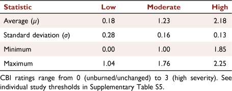
The distribution of field plots classified by burn severity (unburned, low, moderate, high) was provided in 21 studies (a combined 2968 plots). (1) The counts of plots were summed by severity category across studies. In this case, high severity was the most common classification (Fig. 5b); of all field data measured across all studies, there were more high severity plots than any other category. (2) Data were assessed by calculating the proportion of plots placed into different burn severity classes by each study. Here, the highest proportion of plots were in moderate severity areas, followed by high severity, then low severity (Fig. 5c). This means that each study, on average, measured more moderate-severity areas. However, the specific thresholds considered for each severity category varied by study (Table 5).
|
Number of plots per fire and relationship to fire size
For the 357 fires that had recorded plot counts, the average number of plots used per fire was 37.0 (σ = 53.4); 44 fires had no recorded plot counts (Fig. 6a). Both fire size and plot count information were available for 320 fires. The number of plots used per fire increased with fire size, but, as fires get more massive, the plots used increased more slowly (Fig. 6b, log-log slope estimate = 0.2246, P < 0.001, R2 = 0.10).

|
Size and timing of field plots
For the 159 fires where both the date of fire occurrence and timing of field plot measurements were reported, field campaigns occurred 1–40 months after the fire began, with an average delay of 10.5 (σ = 6.0) months (Fig. 7a). Plot size was reported for 137 fires (range = 13–6362 m2, μ = 1331.0 m2, σ = 1734.5; (Fig. 7b). For these fires, plots were mostly circular (105 fires) and sometimes square (32 fires).

|
Spatial distribution of field plots
Most studies located field plots using a stratified approach based on homogenous areas identified by dNBR, as suggested in the FIREMON Landscape Assessment protocol (Key and Benson 2006). However, two studies (Schepers et al. 2014; Warner et al. 2017) located plots in random locations. Schepers et al. (2014) used a split approach, with field measurements in both homogenous and random locations; the randomly located plots were more heterogeneous in both burn severity and vegetation type. Warner et al. (2017) used a random approach combined with relatively many samples, which enabled a simpler and more direct estimate of the accuracy of their remotely sensed severity map.
Remotely sensed data
Remote sensor technologies
The most used sensors were from the Landsat program (Supplementary Table S6). Studies using the Landsat 4–5 (Thematic Mapper; TM) and Landsat 7 (Enhanced Thematic Mapper; ETM+) satellites were the most numerous (60 studies combined), followed by Landsat 8 Operational Land Imager (OLI; 8) and unspecified Landsat sensors (6). Most studies relied on sensors that acquired multispectral imagery with wavelengths encompassing the visible, near infrared, shortwave infrared, and thermal regions of the electromagnetic spectrum (56). Other sensors did not sample at higher wavelengths and thus did not collect shortwave infrared or thermal data. Two studies used Synthetic-aperture radar (SAR). Sensors were mounted on platforms ranging from satellites to airplanes to uncrewed aerial vehicles (UAVs).
Resolution of remotely sensed data
Because the most used sensors were from the Landsat program, most studies used remotely sensed data with a 30 m spatial resolution. The coarsest spatial resolution (1000 m) was associated with the Moderate Resoltion Imaging Spectroradiometer (MODIS) on NASA Terra and Aquas satellites (Holden et al. 2010; Kolden and Rogan 2013; Hultquist et al. 2014; Zheng et al. 2016), and the finest (0.02 m) was from imagery collected by a consumer-grade RGB camera (Fraser et al. 2017).
Number of sensors used and inclusion of single or bitemporal data
Most studies used a single sensor (49) or included two sensors (11) (Supplementary Fig. S3a). Two studies included three or four sensors. For our analysis, all Landsat sensors (TM, ETM+, OLI) were combined, so studies using more than one sensor do not reflect those that used different Landsat satellites for pre/post fire imagery. We identified five ways that studies incorporated two or more sensors in their analysis (Table 6). All studies that used more than one sensor included data from at least one of the Landsat satellites. All but one study that used multiple sensors also collected optical and sometimes also thermal data. The exception was Tanase et al. (2015a), who included both optical and SAR data.

|
Regarding single and bitemporal remotely sensed data, studies mostly included bitemporal imagery (38) (Supplementary Fig. S3b). Sixteen studies that included bitemporal data also analysed relationships using single-date indices. The least common strategy was to include only single-date indices (8); three of these were based on Multiple Endmember Spectral Mixture Analysis.
Atmospheric corrections (absolute radiometric corrections)
The studies reviewed used several atmospheric correction methods for optical data; most common were top of atmosphere (or at-sensor reflectance; 23 studies) or surface reflectance derived by various methods (28) (Supplementary Fig. S4). Eight studies did not specify the level of radiometric correction. Of those, two stated only that radiometric corrections were used, and three stated only that atmospheric corrections were used. Of the studies using surface reflectance, the most commonly stated method was Dark Object Subtraction (DOS; 9), followed by the cosine of the solar zenith angle correction (COST; 4) (Chavez 1996). Other studies used unspecified surface reflectance (15) or used different methods depending on which band was assessed (1). One study quantified the effect of using four atmospheric correction methods (Fang and Yang 2014).
Relative radiometric normalisation
Some bi-temporal datasets used pseudo-invariant features (PIFs) to conduct radiometric normalisation or assess its necessity (10 studies). Most commonly, studies that conducted relative radiometric normalisation used PIFs to regress the pre-fire values against the post-fire values (4), but normalisation of post-fire reflectance to the pre-fire image also occurred (1). The remaining studies that identified PIFs found that no further relative radiometric normalisation was required (5). Except for one case, there was no mention of how PIFs were located; that particular study specified that its method used the iteratively re-weighted multivariate alteration detection (IR-MAD) algorithm to select PIFs, which were then used to normalise the target images on a band-wise basis. The other studies that did not identify PIFs stated that no scene-to-scene radiometric normalisation was applied (2) or used pre-processed imagery prepared by the Monitoring Trends in Burn Severity (MTBS), Burned Area Emergency Response (BAER), or Rapid Assessment of Vegetation Condition after Wildfire (RAVG) programs (5). The remaining 43 studies did not evaluate the need for relative radiometric normalisation.
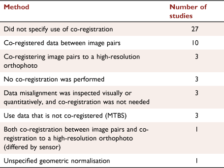
Georeferencing/co-registration
Georeferencing/co-registration was used in some bitemporal datasets to reduce geometric error between image pairs (Table 7). Studies usually did not specify any type of georeferencing or co-registration (27 studies). For the studies that explicitly stated that they did use co-registration, the most common method was to co-register data between image pairs (10). For methods used in the remaining studies, see Table 7.
|
Most studies that undertook co-registration used ground control points to tie images together (specifying 30, 34, 40, 80, or enough control points to achieve specified root-mean-square error [RMSE; 5 studies]). One study used the Imagine Autosync feature in ERDAS Imagine 2015 software (Hexagon Geospatial Inc., Norcross, GA, USA), which matches images using automatically generated tie-points. Studies that reported the accuracy of co-registration (6) did so using either pixel accuracy or RMSE. Pixel accuracy was reported within 0.5 pixels (1) or 1 pixel (1); RMSE was reported using pixel units (4) at levels of 0.014, 0.16, 0.5 or lower, and 0.5. Transformations used included first-order (2), second-order (3), and third-order (1) polynomials. Resampling methods reported were nearest neighbour (2) and bilinear (1).
Types of indices
Most indices used in the studies reviewed were based on the optical region of the electromagnetic spectrum, which incorporates portions of the visible, infrared, and shortwave infrared regions (Fig. 8a). Less common were mixed indices, combining spectral regions with thermal indices, followed by thermal- and radar-based indices. Regarding temporal form, indices were mostly single-date or bitemporal using an absolute (pre-post) difference (Fig. 8b). Less common were relativised bitemporal indices (e.g. RdNBR, RBR). Finally, the least used types of temporal indices were bitemporal ratio indices (pre/post) (2 indices: Radar Burn Ratio, image ratioing) and combination bitemporal absolute difference and single-date index (1 index: dNBR-Enhanced Vegetation Index [EVI]).

|
NBR and Normalised Difference Vegetation Index (NDVI) were among the most studied spectral indices. The top three indices were based on NBR: dNBR (50 studies), followed by RdNBR (25), and NBR (19) (Fig. 8c). The next most common indices were the differenced NDVI (dNDVI, 18 studies) and NDVI (12). Although 105 indices were related to CBI, most appeared in only one or two studies (76 indices; see Supplementary Table S6).
Number of indices per study and combinations of temporal form
The mean number of indices used in each study was 5.0 (σ = 5.7), with up to 26 indices in a single study (Fig. 9a). Absolute difference pre/post-fire indices were the most common (50 studies), followed by relativised bi-temporal indices (26), single-date post-fire indices (23), and ratio indices (3). Most commonly, studies included only absolute indices (21, Fig. 9b). Many studies had both absolute and relativised indices (13); absolute, relativised, and single-date indices (10); or just single-date indices (8). Less commonly, studies reported a combination of single and absolute indices (4) or only relativised indices (3). Least used were absolute, single-date, and ratio indices; absolute and ratio indices; or just ratio indices (1 study each).

|
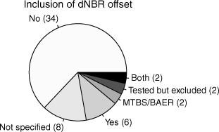
dNBR offset
Most of the studies reviewed (54 of 62) included dNBR as a spectral index. However, the majority of those studies (34) did not include a dNBR offset value (Fig. 10). We found that eight studies did not specify whether an offset value was included or not. Six studies did explicitly state that an offset was included. Additionally, two studies provided analyses both with and without an offset, and two other studies tested whether including an offset value improved the relationship with field data but ultimately excluded it from their analyses. Finally, two studies used MTBS/BAER data, which include an offset value for RdNBR indices, but not in the calculation of dNBR.
|
Pixel value extraction methods
Many studies (22) did not specify how the value of indices for field plots was determined (Table 8). The studies that did specify their method most commonly extracted the value of the pixel over plot centre (14), used a 3 × 3 focal mean window centred on the plot (12), or bilinear smoothing (7). For smoothing types used in the remaining 9 studies, see Table 8.

|
Only two studies quantitatively compared different smoothing methods; one compared bilinear with no smoothing (Stambaugh et al. 2015), and one used four methods for Quickbird imagery in their comparison with ASTER and Landsat data (Holden et al. 2010).
Linking models
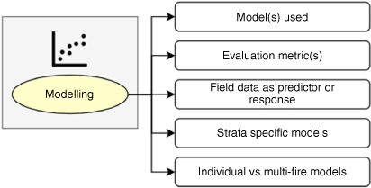
Model(s) used and field data as predictor or response
Fifteen classes of models were used in analyses (Table 9); the most common was linear regression (36 comparisons), followed by quadratic regression (17), and exponential models (9). For the models used in the remaining 30 comparisons, see Table 9.

|
Field data were much more commonly used as a predictor variable (75 comparisons) than as a response variable (19). This pattern held across almost all general model types. However, for three models, field data were used solely as a response variable: the natural logarithm model, the exponential models, and the sigmoidal model. For cubic and unspecified non-linear models, the same number of comparisons used field data as a predictor variable and a response variable. Eight analyses just reported correlation statistics between the two observation methods.
Model performance metrics
Many methods were used to assess or quantify the performance of models that related remotely sensed data to field plots (Table 10). The most common metric was R2 (46 studies), followed by RMSE (17), R2adj (14), p (13), and r (13). Most studies used a single evaluation metric (24) or two metrics (27, Supplementary Fig. S5). Eleven studies assessed three or four metrics.

|
Field plot measurements by strata
The CBI rating encompasses five vegetation strata, commonly separated into understorey (A–C) and overstorey (D, E) components (Fig. 1). Of the 62 studies reviewed, 14 modelled CBI across strata. Three methods investigated whether relationships between field observations and remotely sensed data varied by strata (Table 11). The most common method separately modelled the understorey components (A–C), overstorey components (C, D), and overall severity (5 studies). Studies also modelled each individual stratum separately (4), or modelled the soil or substrate component (A) and surface or vegetation components (B–E), as well as the composite or overall severity (3 studies). Only two studies modelled just the overstorey components (D, E) and overall severity.

|
Single-fire vs multi-fire models
Most studies analysed single-fire local models (33); i.e. relationships between field plots and remotely sensed data were fire-specific (Supplementary Fig. S6). Other studies investigated regional models (19), combined field plots across multiple fires, or evaluated both local and regional models (10).
Discussion
This review highlights the many ways that continuous measures of severity, based on the CBI, have been linked to remotely sensed data, and outlines the range of methods and decisions in the process. Five main topics were investigated: (1) study information; (2) fire data; (3) field data; (4) remotely sensed data; and (5) linking models. Overall, we found wide variability in the methodological decisions and analytical tools used by the included studies. This finding raises the challenge of knowing whether differences among study results are driven by site-specific ecological and fire differences or were affected by differences in the methodological approaches. One outcome of this study was to provide flowcharts that highlight decisions that can be made during field data collection, remotely sensed data collection, and modelling phases (Figs 11–13). These flowcharts may facilitate more comparative studies that assess the robustness of the workflow to differences in methodological choices and highlight potential future research directions. Combined with the breakdown of methods and number of studies that have investigated each decision, future studies may focus on specific areas of the analytical framework that are not well represented (such as the effectiveness of thermal, radar, and lidar data compared with spectral imagery), or they may seek to conduct more extensive meta-analyses comparing multiple methodological choices. Additionally, we found several key research gaps that warrant future investigation. Finally, we encourage future studies to provide explicit description and justification behind their methodological approaches to make comparisons among findings in separate studies more possible.

|

|
|
Comparative investigations
There is no one consensus for the best way to connect field observations to remotely sensed data, and uncertainties exist at every decision point. First of all, there is no universal, one-size-fits-all approach to evaluating burn severity (Cocke et al. 2005; Keeley 2009). Although some studies suggest more utility, and that tree-level measurements that directly assess ecological effects may be preferable to a composite index that aggregates semi-quantitative estimates of change across a plot (Morgan et al. 2014; Furniss et al. 2020), the choice of assessment should be determined by management, ecological purposes, and field sampling designs (Ryan and Noste 1985). We identified, where available, analyses that compared important decision points in linking field observations of CBI as a continuous variable to remotely sensed data. The numerous analytical decisions and paths that studies applied prevented strong generalisations from being made, especially considering that relatively few studies compared multiple approaches at key decision points in the workflow. Of those that did, many returned mixed results. Consequentially, the choice of how burn severity is measured and modelled influences study outcomes.
One such example relates to the comparison of different composite severity measures (CBI, GeoCBI, and WCBI). Three studies (De Santis and Chuvieco 2009; Cansler and McKenzie 2012; Mallinis et al. 2018) compared multiple ground measures of severity and found that no one method seemed to result in the greatest correspondence between field- and satellite-based estimates of burn severity across different regions. For both Cansler and McKenzie (2012) and Mallinis et al. (2018), who both included analysis of CBI, GeoCBI, and WCBI, the best performing field measurement depended on which spectral index (and in the case of Mallinis et al. (2018), which sensor) was used. De Santis and Chuvieco (2009) compared CBI and GeoCBI, and found that GeoCBI peformed best for two of the three fires assessed, and CBI performed best on the third. Thus, although metrics of fractional cover, leaf area index, or other weighting approaches did in some cases improve burn severity models, the mixed results failed to provide a convincing answer as to which composite severity measure is best.
Another example of the lack of consensus about how to sample fires relates to the inclusion of unburned and low-severity field plots in the field sample set, which provides an anchor at the low range of CBI for assessing relationships with remotely sensed data. The bias that we identified of field plots tending towards moderate- and high-severity areas likely occurs for two reasons: (1) attempts to overcome the saturation of remotely sensed indices at high severities (van Wagtendonk et al. 2004; De Santis et al. 2010; Veraverbeke et al. 2012; Parks et al. 2014); and (2) the importance of these areas to management (Robichaud 2000; Miller and Thode 2007; French et al. 2008; Cansler and McKenzie 2012; Fernández-García et al. 2018b). We found substantial variation in the thresholds used in classification, but it was clear that the underrepresentation of lower range of severities occurred despite that variation. The fact that only one of the two studies that excluded unburned plots from their analysis (Murphy et al. 2008) provided a rationale (the unburned sites (CBI = 0) disproportionately influenced the linear fit to produce remaining non-liner residual structure) highlights the need for more comparative analyses in this realm.
These examples highlight the uncertainty that often remains following quantitative assessments of methodological approaches. This is not unique to methods based on composite severity indices, however – Furniss et al. (2020) found that estimates of tree-level metrics such as mortality of stems and basal area could vary widely for a single spectral index value. Such uncertainties are unsatisfying and provide reason for caution when applying methodologies developed in one context, for example based on a single fire or ecosystem type, outside the scope of inference. For example, some influential studies (like Cansler and McKenzie’s (2012) comparison of multiple pixel value extraction methods) are widely cited by subsequent investigators but without validating their effectiveness in subsequent studies or in new regions. However, such studies may be highly site- and context-specific, and it is unclear how broadly applicable their results are. In other cases, attempts to compare different approaches, such as using sensors with varying spatial resolution, are confounded by lurking variables – in this case, the spectral resolution of different sensors and the spatial synchrony with field plots (van Wagtendonk et al. 2004; Holden and Evans 2010; Tanase et al. 2015a; Mallinis et al. 2018; García-Llamas et al. 2019). While several of these studies found slight improvements for sensors with high spatial resolution compared with Landsat imagery (Holden and Evans 2010; Mallinis et al. 2018; García-Llamas et al. 2019), it is difficult to disentangle their results to isolate the effects of the spatial resolution of the sensors. Finally, there may not yet exist any comparative studies in the current literature assessing the effect of georeferencing remotely sensed data on model results. Although 27 of 62 studies conducted or investigated the need for georeferencing (or co-registration between image pairs), no studies presented comparative analysis of the impacts on model results.
Realistically, only studies that replicate their methodological approach (e.g. use similar methods of collecting field observations, include unburned field plots, extract pixel values over plot centre with the same method, etc.) can be compared across each other. It is not well-quantified what level of uncertainty arises in comparing results across different studies where methodologies were not consistent. Therefore, more broad-scale comparative studies are needed to understand the transferability of methods across landscapes and methods/technologies.
Compounding uncertainty
Studies have investigated individual slices of the ‘decision menu’ (i.e. the many potential analytical approaches to a particular step in the analysis; Fig. 2), but none have looked at how uncertainty compounds across the whole analysis process from beginning to end. Stambaugh et al. (2015) assessed the compounding uncertainty across three decision points: (1) two index value extraction methods (none and bilinear interpolation); (2) two timings of remotely sensed data (initial vs extended assessment); and (3) two spectral indices (dNBR vs RdNBR). Their analysis thus followed 23 = 8 different pathways and showed that R2 for models of overall CBI values ranged from 0.03 to 0.61. This study demonstrates the importance of understanding not just how each slice of the decision menu can affect model results but also how those uncertainties can be compounded through different analytical pathways. Additionally, because many of the comparative studies discussed above provide mixed results when looking at a single decision point, it is unclear how important such choices are at the global scale of analysis. A comprehensive study of the many potential analytical approaches would help understand when differences at different decision points wash out and when they do not, allowing us to understand when we are seeing ‘true’ differences among studies and when those are due to differences in the methods used.
Key gaps
We identified several key research gaps or biases in the studies reviewed. The previous sections addressed the importance of comparative studies targeting key points in the ‘decision menu’ of an analysis. Here, we identify where individual studies are absent or lacking from the literature identified in our review.
The uneven distribution in the types and locations of fires studied has important implications for how widely applicable the results are across different fires and geographies in the future. First, most fires were wildfires, with some prescribed and wildland fire use fires. Although this makes sense from a perspective of pre-fire management and post-fire intervention, there is reason to question whether prescribed fires behave in fundamentally different ways than wildfire. For example, Arkle and Pilliod (2010) found that prescribed fires did not mimic the ecological effects that followed wildfire in a riparian ecosystem; both the extent and severity of vegetation burned was substantially lower in the prescribed fire compared with nearby wildfires. How severity models based on remotely sensed data under such conditions might differ remains unclear. Some landscapes, such as those in the southeast USA, experience primarily prescribed fires – where resources for post-fire assessment may be more heavily allocated to determining if the burn objectives were successfully achieved. In those cases, the CBI protocol may be overly broad, and other, more direct measures of ecosystem change may be preferred (Morgan et al. 2014).
Second, there was a heavy geographical bias towards the USA and especially western USA, as well as a heavy focus on temperate coniferous forests. These results reflect that western USA (1) has a long history of wildfire research; (2) experiences large fires in many forested areas; and (3) has high spatial variability in fire regimes and biodiversity (Heyerdahl et al. 2001; Morgan et al. 2001). However, the concentration of fire research in this area may also mean that major swathes of ecosystems elsewhere are unstudied. Non-forested areas, such as frequently burning grasslands, aren’t suitable for assessments with CBI (i.e. it is difficult to classify burn severity as anything other than burned and unburned). However, some regions that are forested and experience frequent fires or have extensive fire histories (e.g. Italy, France, Indonesia, or Brazil) are not highly represented by CBI studies. One reason for this could be different research traditions or regional research history. For example, in Australia, alternative visual estimation approaches have been used (Hammill and Bradstock 2006; Chafer 2008) instead of CBI. A second reason may be due to differences in the underlying ecology of post-fire responses. For example, some forests grow back in very different ways (e.g. resprouting eucalypts) compared with temperate and boreal forests, where CBI was originally developed. Although other regions may have different ways of conducting field estimates of severity not included in this review, the ability to make comparisons between those studies and CBI is limited.
The limited range in the size and timing of field plot collection limits our understanding of how field data at different scales affects model variability and of long-term ecosystem change. First, there was a strong bias towards 30-m diameter plots, raising the question of what spatial scales are missing in current analyses. The CBI was initially designed with 30-m diameter plots to match the spatial grain of imagery collected by the Landsat satellite program (Eidenshink et al. 2007), but has since been adapted and related to many different sensors of both higher and lower resolution (Supplementary Table S6). Second, we found a relative lack of more extended intervals between fire occurrence and field data collection (on the order of 3–10 years post-fire), as well as an absence of studies conducting repeated measurements.
Although the collection of field data is often limited by site accessibility, high costs, and time constraints (Chuvieco et al. 2006; Boucher et al. 2017), there are clearly opportunities for studies that sample outside the range of commonly used field plot sizes and timing delays. For example, studies could collect very large field plots (e.g. 250 m diameter); however, such an endeavour might take weeks to months, and environmental factors such as rain or wind could affect measurements (Meng and Meentemeyer 2011). It remains unclear how sampling very large field plots may impact relationships with remotely sensed data, especially those of relatively coarse spatial resolution. Additionally, studies could collect plots at extended times post-fire. However, it becomes more difficult to see burn severity effects on the ground. Most studies conform to the 1–2 year time frame of ‘initial’ and ‘extended’ assessments described by Key and Benson (2006), and the effectiveness of the CBI protocols over extended time-periods has not been well studied. This could be because burned areas can become very hazardous to assess because of falling trees and branches, making access challenging over time.
The 15 model forms used across the studies begs the question of how robust results are to uncertainty in model form. The sheer number of model forms in the studies reviewed shows the diversity of statistical approaches used to link remotely sensed data to field observations. We identified two main considerations in the choice of model form: (1) the behaviour of remote sensor and ecosystem considerations (sensor saturation, nonlinearity at high severities); and (2) model performance (based on evaluation metrics). Although studies such as van Wagtendonk et al. (2004) modelled CBI using a quadratic model, the predicted reduction in CBI at high dNBR values is not an expected behaviour of the sensor-ecosystem dynamic (Hall et al. 2008). Thus, some studies argued for nonlinear models with saturated growth characteristics (e.g. CBI = dNBR × (a[dNBR] + b)−1; Hall et al. 2008), even when this choice is not strictly supported by model evaluation metrics. The motivations for selecting different model forms were seldom described, but many studies clearly tried to find the best descriptor of the observed relationship. In studies that considered the sensor-ecosystem dynamic, predicting a trend that is feasible in the real world overrode the aim for strong performance (Hall et al. 2008; Boucher et al. 2017). That said, studies rarely compared more than a few models, and the robustness of relationships to uncertainty in model form is not well understood.
Finally, the mixed results in the 14 of 62 studies that modelled CBI across strata demonstrated that conceptual models of remote sensed data reported strengths or weaknesses in correlating with specific burn severity measures that would not be expected from theory. Specifically, we identified some studies showed stronger relationships in lower canopy strata – in conflict with accepted theory that passive remotely sensed data are limited by low signal penetration (Chen et al. 2015) and disproportionately capture changes in the upper canopy (Kasischke et al. 2008). Several studies support the theory that passive sensors are more likely to detect fire effects in the upper part of the vegetation stratum (Patterson and Yool 1998; Hudak et al. 2004; De Santis and Chuvieco 2009). Conceptually, the ability to capture change in lower canopy strata is impacted by vegetation density, because burned landscapes may reflect more changes in the overstorey strata due to the shielding effect of vegetation or their remains (Soverel et al. 2011; Tanase et al. 2011). Although relationships between field observations and remotely sensed data were generally strong in the overstorey components, large tree stratum, and vegetation components (Chen et al. 2011, 2015; Meng and Meentemeyer 2011; Stambaugh et al. 2015; Wu et al. 2015; Warner et al. 2017), two studies found that the understorey components outperformed higher canopy strata (Hoy et al. 2008; Tanase et al. 2011). These exceptions to the conceptual rule-of-thumb that passive remotely sensed data are limited in their ability to detect change in lower canopy strata deserve more scrutiny and better understanding of the conditions under which lower forest strata may be observed.
Importance of providing rationales
Our research highlighted the importance – especially given the lack of consensus on analytical methods – of providing rationales for each decision in the analysis workflow that link back to the research objectives. For example, in regards to the two previously stated considerations that drove the choice of model form in the reviewed studies, it would be beneficial for future investigators to more explicitly give the rationale behind their model selection methods and state the conditions under which those models can be appropriately interpreted. Choosing to sacrifice model performance for predictions that correspond to expected behaviour of the sensor and ecosystem dynamic may create difficult comparisons across fires or regions, but it also provides considerable benefit in that they reflect the true nature of the system. Both approaches are equally valid given conforming research objectives, but we suggest that studies (1) consider the purpose of their analysis when determining appropriate models to assess and (2) convey whether weaker model performance metrics may result from their decisions.
Similarly, we found that studies did not always state their rationale for using field data as either predictor or response variables depending on their research objectives. In typical regression analysis, a causal relationship is implied between one or more predictors, and a response (Bordacconi and Larsen 2014). Cansler and McKenzie (2012) used this logic to argue for CBI as a predictor variable, because burn severity changes reflectance, not the other way around. They further stated that CBI has the greatest certainty associated with its meaning and thus should be used to predict the variables with no inherent ecological meaning (e.g. dNBR or RdNBR). Conversely, in some cases CBI (or other ground severity measure) may serve as a response variable, with remotely sensed data serving as the predictor variable if the main study goal is to predict severity on the ground (Zhu et al. 2006). In these cases, studies taking this approach follow the logic that the known value in a satellite image (e.g. RdNBR) is the predictor variable being used to model the unknown value on the ground (e.g. tree mortality) as the response variable. Both approaches have their benefits and challenges, though readers could benefit from more studies explicitly describing when and why field data are considered as predictor versus response variables, because model configuration affects the ability to compare across studies.
The analytical process of modelling of continuous composite severity measures using remotely sensed data can be split into three main phases: (1) collection of field data; (2) collection of remotely sensed data; and (3) modelling. We provide figures that break down the main decisions that can be made at each phase (Figs 11–13). This blueprint for preparation and analysis should be useful for considering key decisions in study design as well as emphasising the choices that should be justified when reporting study results (see example rationales in Table 12).

|
Study limitations
Many decisions discussed in this paper revolve around image quality and availability, and problems with comparability and synthesis across disparate collections of CBI data result from this limitation. The selection of suitable remotely sensed imagery requires consideration of many different characteristics, including solar zenith angle, atmospheric effects, plant phenology, and the availability of cloud-free imagery (Rogan et al. 2002; Epting et al. 2005; De Santis and Chuvieco 2007; Ju and Roy 2008). If bi-temporal indices are used, then inter-annual meteorological differences (Veraverbeke et al. 2010) and the misregistration of image pixels (Verbyla and Boles 2000) must also be considered. Sensor differences and some atmospheric effects may be corrected through radiometric normalisation methods, but differences in vegetation phenology may be unavoidable, particularly in cloudy regions where there may be few cloud-free images available (Epting et al. 2005). Furthermore, the seasonality and lag timing of post-fire imagery can impact the values of spectral indices. For example, RdNBR is sensitive to ash cover, which declines with time since fire (Miller and Quayle 2015). Therefore, RdNBR values that represent total mortality can be different immediately post-fire compared with the following year. Veraverbeke et al. (2010) provide an in-depth discussion of the effect of seasonal timing on index values.
Although limitations in image availability interact and potentially exacerbate the other problems/limitations that were identified in previous studies, our review focuses on the wider set of methodological practices. Future meta-analyses could focus on CBI datasets that cover broader extents (Picotte et al. 2019) and spectral index processing methods that are less reliant on individual image selection techniques (Parks et al. 2021). Studies using these additional datasets and approaches will likely impact accepted research practices and potentially lead to more consistent methodologies. Currently, researchers may want to consider the effects of those limitations along with other issues we raise in this paper.
One major limitation of this study is that we did not evaluate the specific equations used to calculate each spectral index included in the studies. A few references provide incomplete equations – for example, in the original Miller and Thode (2007) study presenting RdNBR, they do not include multiplying by 1000 explicitly in the equation, nor any modifications needed to deal with 0 in the denominator. Additionally, many studies do not explicitly include the use of offset values in the equation. We captured this information where available but recommend that authors more explicitly state the form of the equations for spectral indices as well as any use of offset values. We did not endeavour to include the correct equations here (Supplementary Table S7), but we note the issue with past inconsistencies.
Many of the North American studies used overlapping CBI datasets (so the datasets are not really independent – e.g. Cansler and McKenzie (2012) data were used by Karau et al. (2014) as well as Parks et al. (Parks et al. 2014, 2018, 2019). We also note that much of the CBI datasets analysed by the papers in this review are available in a data repository for reanalysis (Picotte et al. 2019).
We did not include studies in our review that used direct forest measurements, for example the percentage of tree mortality or char and ash colour (see Table 1). This may have introduced some geographic bias in which studies were excluded because some regions may rely more heavily on severity measurements based on direct, individual metrics. For example, Morgan et al. (2014) recommend recording actual fire measurements that have logical and mechanistic connections to the properties a sensor can detect, avoiding the use of composite measures such as CBI that collapse multiple ecosystem attributes into a single index. Several studies have begun to record direct measures of burn severity rather than CBI only (Whitman et al. 2018; Harvey et al. 2019; Saberi et al. 2022), though detailed field measures of burn severity remain rare compared with the widespread use of CBI. Another alternative approach to characterising burn severity over large areas uses lidar data to more directly measure changes in forest structure (McCarley et al. 2017). Although using multi-temporal lidar to examine changes in forest structure due to fire would allow more precise measurement of individual metrics (e.g. change in canopy cover), reduce observer bias, and allow quantification of change in areas without nearby unburned reference sites, the approach remains limited by the availability of pre- and post-fire lidar at adequate time intervals.
Recommendations
Given the difficulty of synthesising results across studies that used varying methodologies, we support efforts such as Picotte et al. (2019) to aggregate and disseminate datasets based on composite severity field observations from investigators. This could provide the necessary information to conduct a meta-analysis of the effects of compounding error across the ‘decision menu’ presented in this review. Additionally, we recommend future studies complete the following:
Collect and share field data in such a way that the original and modified composite severity measures identified in this review (CBI and GeoCBI/WCBI) could all be calculated, thus facilitating further comparisons among the different field measures. Such a request may require the development of a new CBI field collection form for collection of raw field measurements that could be used to calculate any of these.
Report full detail of any processing and analysis. For this review, we followed up with authors where information was missing; however, we were not able to obtain information requested in every case. For a list of recommended information to report, Table 13.
Report the reasoning for methodological choices at each step in the analysis. One of the goals of this review was to identify key analytical decisions and potential reasons why investigators may want to make one decision vs another (Table 12).

|
Conclusion
This review of studies linking remotely sensed data to continuous measures of burn severity measured with the Composite Burn Index highlights: (1) the wide range in analytical approaches and lack of consensus in methodological decisions; (2) the scarcity of comparative studies at any one point in the ‘decision menu’ and absence of a comprehensive beginning-to-end quantitative analysis of compounding uncertainty throughout the analysis framework; and (3) key gaps in research relating to the distribution in the types and locations of fires studied, limited range in the size and timing of field plot collection, and modelling of CBI across strata.
The results of this review provide a framework for future studies linking remotely sensed data to continuous measures of severity by summarising the key analytical decisions and the distribution of studies using such techniques. We avoid concluding which methods or decisions perform best and instead focus on the importance of understanding the wide varieties of ways this type of research has been done, and its potential impacts on our understanding of the state of the science. We find that much uncertainty remains in light of a lack of comparative analysis and biases in the study designs. In the absence of a consensus approach to modelling severity using remotely sensed data, we suggest future research explicitly state their rationales for each analytical decision and how it relates to their specific research questions.
Supplementary material
Supplementary material is available online.
Data availability
The data that support this study will be shared upon reasonable request to the corresponding author.
Conflicts of interest
The authors declare no conflicts of interest.
Declaration of funding
This work was partially supported by the USDA Forest Service Pacific Northwest Research Station [Agreement Numbers: 17-PA-11261987-043, 20-JV-11261987-035], and the Precision Forestry Cooperative, University of Washington, Seattle, Washington, USA.
Author contributions
Conceptualisation, C. W. M. and B. J. H.; data curation, C. W. M.; formal analysis, C. W. M., funding acquisition, C. W. M, E. A., and L. M. M.; investigation, C. W. M. and B. J. H.; project administration, C. W. M.; resources, C. W. M., E. A., and L. M. M.; software, C. W. M.; supervision, B. J. H., V. R. K, E. A., and L. M. M.; validation, C. W. M.; visualisation, C. W. M.; writing – original draft, C. W. M., writing – review and editing, C. W. M., B. J. H., V. R. K., E. A., and L. M. M. All authors have read and agreed to the published version of the manuscript.
Acknowledgements
We thank Alina Cansler for a review of an earlier version of this manuscript prior to submission. We also thank two anonymous reviewers for their comments that greatly improved the quality of this manuscript.
References
Allen JL, Sorbel B (2008) Assessing the differenced Normalized Burn Ratio’s ability to map burn severity in the boreal forest and tundra ecosystems of Alaska’s national parks. International Journal of Wildland Fire 17, 463–475.| Assessing the differenced Normalized Burn Ratio’s ability to map burn severity in the boreal forest and tundra ecosystems of Alaska’s national parks.Crossref | GoogleScholarGoogle Scholar |
Arkle RS, Pilliod DS (2010) Prescribed fires as ecological surrogates for wildfires: a stream and riparian perspective. Forest Ecology and Management 259, 893–903.
| Prescribed fires as ecological surrogates for wildfires: a stream and riparian perspective.Crossref | GoogleScholarGoogle Scholar |
Bastarrika A, Chuvieco E, Martín MP (2011) Mapping burned areas from Landsat change TM/ETM+ data with a two-phase algorithm: balancing omission and commission errors. Remote Sensing of Environment 115, 1003–1012.
| Mapping burned areas from Landsat change TM/ETM+ data with a two-phase algorithm: balancing omission and commission errors.Crossref | GoogleScholarGoogle Scholar |
Bordacconi MJ, Larsen MV (2014) Regression to causality: regression-style presentation influences causal attribution. Research & Politics 1, 2053168014548092
| Regression to causality: regression-style presentation influences causal attribution.Crossref | GoogleScholarGoogle Scholar |
Boucher J, Beaudoin A, Hébert C, Guindon L, Bauce É (2017) Assessing the potential of the differenced Normalized Burn Ratio (dNBR) for estimating burn severity in eastern Canadian boreal forests. International Journal of Wildland Fire 26, 32–45.
| Assessing the potential of the differenced Normalized Burn Ratio (dNBR) for estimating burn severity in eastern Canadian boreal forests.Crossref | GoogleScholarGoogle Scholar |
CAL FIRE (2020) Fire Perimeters [dataset]. California Department of Forestry and Fire Protection’s Fire and Resource Assessment Program (FRAP). Available at https://frap.fire.ca.gov/mapping/gis-data/
Cansler CA, McKenzie D (2012) How robust are burn severity indices when applied in a new region? Evaluation of alternate field-based and remote-sensing methods. Remote Sensing 4, 456–483.
| How robust are burn severity indices when applied in a new region? Evaluation of alternate field-based and remote-sensing methods.Crossref | GoogleScholarGoogle Scholar |
Chafer CJ (2008) A comparison of fire severity measures: an Australian example and implications for predicting major areas of soil erosion. CATENA 74, 235–245.
| A comparison of fire severity measures: an Australian example and implications for predicting major areas of soil erosion.Crossref | GoogleScholarGoogle Scholar |
Chappell CB, Agee JK (1996) Fire severity and tree seedling establishment in Abies magnifica forests, southern Cascades, Oregon. Ecological Applications 6, 628–640.
| Fire severity and tree seedling establishment in Abies magnifica forests, southern Cascades, Oregon.Crossref | GoogleScholarGoogle Scholar |
Charron I, Greene DF (2002) Post-wildfire seedbeds and tree establishment in the southern mixedwood boreal forest. Canadian Journal of Forest Research 32, 1607–1615.
| Post-wildfire seedbeds and tree establishment in the southern mixedwood boreal forest.Crossref | GoogleScholarGoogle Scholar |
Chavez PS (1996) Image-based atmospheric corrections – revisited and improved. Photogrammetric Engineering and Remote Sensing 62, 1025–1035.
Chen XX, Vogelmann JE, Rollins M, Ohlen D, Key CH, Yang LM, Huang CQ, Shi H (2011) Detecting post-fire burn severity and vegetation recovery using multitemporal remote sensing spectral indices and field-collected composite burn index data in a ponderosa pine forest. International Journal of Remote Sensing 32, 7905–7927.
| Detecting post-fire burn severity and vegetation recovery using multitemporal remote sensing spectral indices and field-collected composite burn index data in a ponderosa pine forest.Crossref | GoogleScholarGoogle Scholar |
Chen G, Metz MR, Rizzo DM, Meentemeyer RK (2015) Mapping burn severity in a disease-impacted forest landscape using Landsat and MASTER imagery. International Journal of Applied Earth Observation and Geoinformation 40, 91–99.
| Mapping burn severity in a disease-impacted forest landscape using Landsat and MASTER imagery.Crossref | GoogleScholarGoogle Scholar |
Choung Y, Lee B-C, Cho J-H, Lee K-S, Jang I-S, Kim S-H, Hong S-K, Jung H-C, Choung H-L (2004) Forest responses to the large-scale east coast fires in Korea. Ecological Research 19, 43–54.
| Forest responses to the large-scale east coast fires in Korea.Crossref | GoogleScholarGoogle Scholar |
Churchill DJ, Larson AJ, Dahlgreen MC, Franklin JF, Hessburg PF, Lutz JA (2013) Restoring forest resilience: from reference spatial patterns to silvicultural prescriptions and monitoring. Forest Ecology and Management 291, 442–457.
| Restoring forest resilience: from reference spatial patterns to silvicultural prescriptions and monitoring.Crossref | GoogleScholarGoogle Scholar |
Churchill DJ, Jeronimo SMA, Hessburg PF, Cansler CA, Povak NA, Kane VR, Lutz JA, Larson AJ (2022) Post-fire landscape evaluations in Eastern Washington, USA: assessing the work of contemporary wildfires. Forest Ecology and Management 504, 119796
| Post-fire landscape evaluations in Eastern Washington, USA: assessing the work of contemporary wildfires.Crossref | GoogleScholarGoogle Scholar |
Chuvieco E, Riaño D, Danson FM, Martin P (2006) Use of a radiative transfer model to simulate the postfire spectral response to burn severity. Journal of Geophysical Research: Biogeosciences 111, G04S09
| Use of a radiative transfer model to simulate the postfire spectral response to burn severity.Crossref | GoogleScholarGoogle Scholar |
Cocke AE, Fulé PZ, Crouse JE (2005) Comparison of burn severity assessments using Differenced Normalized Burn Ratio and ground data. International Journal of Wildland Fire 14, 189–198.
| Comparison of burn severity assessments using Differenced Normalized Burn Ratio and ground data.Crossref | GoogleScholarGoogle Scholar |
De Santis A, Chuvieco E (2007) Burn severity estimation from remotely sensed data: performance of simulation versus empirical models. Remote Sensing of Environment 108, 422–435.
| Burn severity estimation from remotely sensed data: performance of simulation versus empirical models.Crossref | GoogleScholarGoogle Scholar |
De Santis A, Chuvieco E (2009) GeoCBI: a modified version of the Composite Burn Index for the initial assessment of the short-term burn severity from remotely sensed data. Remote Sensing of Environment 113, 554–562.
| GeoCBI: a modified version of the Composite Burn Index for the initial assessment of the short-term burn severity from remotely sensed data.Crossref | GoogleScholarGoogle Scholar |
De Santis A, Asner GP, Vaughan PJ, Knapp DE (2010) Mapping burn severity and burning efficiency in California using simulation models and Landsat imagery. Remote Sensing of Environment 114, 1535–1545.
| Mapping burn severity and burning efficiency in California using simulation models and Landsat imagery.Crossref | GoogleScholarGoogle Scholar |
Dillon GK, Holden ZA, Morgan P, Crimmins MA, Heyerdahl EK, Luce CH (2011) Both topography and climate affected forest and woodland burn severity in two regions of the western US, 1984 to 2006. Ecosphere 2, 130
| Both topography and climate affected forest and woodland burn severity in two regions of the western US, 1984 to 2006.Crossref | GoogleScholarGoogle Scholar |
Doerr SH, Shakesby RA, Blake WH, Chafer CJ, Humphreys GS, Wallbrink PJ (2006) Effects of differing wildfire severities on soil wettability and implications for hydrological response. Journal of Hydrology 319, 295–311.
| Effects of differing wildfire severities on soil wettability and implications for hydrological response.Crossref | GoogleScholarGoogle Scholar |
Eidenshink J, Schwind B, Brewer K, Zhu ZL, Quayle B, Howard S (2007) A project for monitoring trends in burn severity. Fire Ecology 3, 3–21.
| A project for monitoring trends in burn severity.Crossref | GoogleScholarGoogle Scholar |
Epting J, Verbyla D, Sorbel B (2005) Evaluation of remotely sensed indices for assessing burn severity in interior Alaska using Landsat TM and ETM+. Remote Sensing of Environment 96, 328–339.
| Evaluation of remotely sensed indices for assessing burn severity in interior Alaska using Landsat TM and ETM+.Crossref | GoogleScholarGoogle Scholar |
Escuin S, Navarro R, Fernández P (2008) Fire severity assessment by using NBR (Normalized Burn Ratio) and NDVI (Normalized Difference Vegetation Index) derived from LANDSAT TM/ETM images. International Journal of Remote Sensing 29, 1053–1073.
| Fire severity assessment by using NBR (Normalized Burn Ratio) and NDVI (Normalized Difference Vegetation Index) derived from LANDSAT TM/ETM images.Crossref | GoogleScholarGoogle Scholar |
Fang L, Yang J (2014) Atmospheric effects on the performance and threshold extrapolation of multi-temporal Landsat derived dNBR for burn severity assessment. International Journal of Applied Earth Observation and Geoinformation 33, 10–20.
| Atmospheric effects on the performance and threshold extrapolation of multi-temporal Landsat derived dNBR for burn severity assessment.Crossref | GoogleScholarGoogle Scholar |
Fernández-García V, Quintano C, Taboada A, Marcos E, Calvo L, Fernández-Manso A (2018a) Remote sensing applied to the study of fire regime attributes and their influence on post-fire greenness recovery in pine ecosystems. Remote Sensing 10, 733
| Remote sensing applied to the study of fire regime attributes and their influence on post-fire greenness recovery in pine ecosystems.Crossref | GoogleScholarGoogle Scholar |
Fernández-García V, Santamarta M, Fernández-Manso A, Quintano C, Marcos E, Calvo L (2018b) Burn severity metrics in fire-prone pine ecosystems along a climatic gradient using Landsat imagery. Remote Sensing of Environment 206, 205–217.
| Burn severity metrics in fire-prone pine ecosystems along a climatic gradient using Landsat imagery.Crossref | GoogleScholarGoogle Scholar |
Fraser RH, Van der Sluijs J, Hall RJ (2017) Calibrating satellite-based indices of burn severity from UAV-derived metrics of a burned boreal forest in NWT, Canada. Remote Sensing 9, 279
| Calibrating satellite-based indices of burn severity from UAV-derived metrics of a burned boreal forest in NWT, Canada.Crossref | GoogleScholarGoogle Scholar |
French NHF, Kasischke ES, Hall RJ, Murphy KA, Verbyla DL, Hoy EE, Allen JL (2008) Using Landsat data to assess fire and burn severity in the North American boreal forest region: an overview and summary of results. International Journal of Wildland Fire 17, 443–462.
| Using Landsat data to assess fire and burn severity in the North American boreal forest region: an overview and summary of results.Crossref | GoogleScholarGoogle Scholar |
Furniss TJ, Kane VR, Larson AJ, Lutz JA (2020) Detecting tree mortality with Landsat-derived spectral indices: improving ecological accuracy by examining uncertainty. Remote Sensing of Environment 237, 111497
| Detecting tree mortality with Landsat-derived spectral indices: improving ecological accuracy by examining uncertainty.Crossref | GoogleScholarGoogle Scholar |
García-Llamas P, Suárez-Seoane S, Fernández-Guisuraga JM, Fernández-García V, Fernández-Manso A, Quintano C, Taboada A, Marcos E, Calvo L (2019) Evaluation and comparison of Landsat 8, Sentinel-2 and Deimos-1 remote sensing indices for assessing burn severity in Mediterranean fire-prone ecosystems. International Journal of Applied Earth Observation and Geoinformation 80, 137–144.
| Evaluation and comparison of Landsat 8, Sentinel-2 and Deimos-1 remote sensing indices for assessing burn severity in Mediterranean fire-prone ecosystems.Crossref | GoogleScholarGoogle Scholar |
Greene DF, Noël J, Bergeron Y, Rousseau M, Gauthier S (2004) Recruitment of Picea mariana, Pinus banksiana, and Populus tremuloides across a burn severity gradient following wildfire in the southern boreal forest of Quebec. Canadian Journal of Forest Research 34, 1845–1857.
| Recruitment of Picea mariana, Pinus banksiana, and Populus tremuloides across a burn severity gradient following wildfire in the southern boreal forest of Quebec.Crossref | GoogleScholarGoogle Scholar |
Hall RJ, Freeburn JT, De Groot WJ, Pritchard JM, Lynham TJ, Landry R (2008) Remote sensing of burn severity: experience from western Canada boreal fires. International Journal of Wildland Fire 17, 476–489.
| Remote sensing of burn severity: experience from western Canada boreal fires.Crossref | GoogleScholarGoogle Scholar |
Hammill KA, Bradstock RA (2006) Remote sensing of fire severity in the Blue Mountains: influence of vegetation type and inferring fire intensity. International Journal of Wildland Fire 15, 213–226.
| Remote sensing of fire severity in the Blue Mountains: influence of vegetation type and inferring fire intensity.Crossref | GoogleScholarGoogle Scholar |
Harvey BJ, Donato DC, Turner MG (2014) Recent mountain pine beetle outbreaks, wildfire severity, and postfire tree regeneration in the US Northern Rockies. Proceedings of the National Academy of Sciences 111, 15120–15125.
| Recent mountain pine beetle outbreaks, wildfire severity, and postfire tree regeneration in the US Northern Rockies.Crossref | GoogleScholarGoogle Scholar |
Harvey BJ, Andrus RA, Anderson SC (2019) Incorporating biophysical gradients and uncertainty into burn severity maps in a temperate fire-prone forested region. Ecosphere 10, e02600
| Incorporating biophysical gradients and uncertainty into burn severity maps in a temperate fire-prone forested region.Crossref | GoogleScholarGoogle Scholar |
Heyerdahl EK, Brubaker LB, Agee JK (2001) Spatial controls of historical fire regimes: a multiscale example from the interior west, USA. Ecology 82, 660–678.
| Spatial controls of historical fire regimes: a multiscale example from the interior west, USA.Crossref | GoogleScholarGoogle Scholar |
Holden ZA, Evans JS (2010) Using fuzzy C-means and local autocorrelation to cluster satellite-inferred burn severity classes. International Journal of Wildland Fire 19, 853–860.
| Using fuzzy C-means and local autocorrelation to cluster satellite-inferred burn severity classes.Crossref | GoogleScholarGoogle Scholar |
Holden ZA, Morgan P, Smith AMS, Vierling L (2010) Beyond Landsat: a comparison of four satellite sensors for detecting burn severity in ponderosa pine forests of the Gila Wilderness, NM, USA. International Journal of Wildland Fire 19, 449–458.
| Beyond Landsat: a comparison of four satellite sensors for detecting burn severity in ponderosa pine forests of the Gila Wilderness, NM, USA.Crossref | GoogleScholarGoogle Scholar |
Hoy EE, French NHF, Turetsky MR, Trigg SN, Kasischke ES (2008) Evaluating the potential of Landsat TM/ETM+ imagery for assessing fire severity in Alaskan black spruce forests. International Journal of Wildland Fire 17, 500–514.
| Evaluating the potential of Landsat TM/ETM+ imagery for assessing fire severity in Alaskan black spruce forests.Crossref | GoogleScholarGoogle Scholar |
Hudak AT, Robichaud P, Evans JS, Clark J, Lannom K, Morgan P, Stone C (2004) Field validation of Burned Area Reflectance Classification (BARC) products for post fire assessment. In ‘Remote Sensing for Field Users. Proceedings of the 10th Forest Service Remote Sensing Applications Conference, 5–9 April 2004, Salt Lake City, UT’. (Ed. JD Greer) (American Society of Photogrammetry and Remote Sensing: Bethesda, MD, USA)
Hultquist C, Chen G, Zhao K (2014) A comparison of Gaussian process regression, random forests and support vector regression for burn severity assessment in diseased forests. Remote Sensing Letters 5, 723–732.
| A comparison of Gaussian process regression, random forests and support vector regression for burn severity assessment in diseased forests.Crossref | GoogleScholarGoogle Scholar |
Isaev AS, Korovin GN, Bartalev SA, Ershov DV, Janetos A, Kasischke ES, Shugart HH, French NHF, Orlick BE, Murphy TL (2002) Using remote sensing to assess Russian forest fire carbon emissions. Climatic Change 55, 235–249.
| Using remote sensing to assess Russian forest fire carbon emissions.Crossref | GoogleScholarGoogle Scholar |
Jain TB, Graham RT (2004) Is forest structure related to fire severity? Yes, no, maybe: methods and insights in quantifying the answer. In ‘Silviculture in Special Places: Proceedings of the National Silviculture Workshop, Granby, CO, USA’. (Eds WD Shepperd, LG Eskew) RMRS-P-34. pp. 217–234. (USDA Forest Service Rocky Mountain Research Station: Fort Collins, CO, USA)
Johnstone JF, Chapin FS (2006) Effects of soil burn severity on post-fire tree recruitment in boreal forest. Ecosystems 9, 14–31.
| Effects of soil burn severity on post-fire tree recruitment in boreal forest.Crossref | GoogleScholarGoogle Scholar |
Ju J, Roy DP (2008) The availability of cloud-free Landsat ETM+ data over the conterminous United States and globally. Remote Sensing of Environment 112, 1196–1211.
| The availability of cloud-free Landsat ETM+ data over the conterminous United States and globally.Crossref | GoogleScholarGoogle Scholar |
Karau EC, Keane RE (2010) Burn severity mapping using simulation modelling and satellite imagery. International Journal of Wildland Fire 19, 710–724.
| Burn severity mapping using simulation modelling and satellite imagery.Crossref | GoogleScholarGoogle Scholar |
Karau EC, Sikkink PG, Keane RE, Dillon GK (2014) Integrating satellite imagery with simulation modeling to improve burn severity mapping. Environmental Management 54, 98–111.
| Integrating satellite imagery with simulation modeling to improve burn severity mapping.Crossref | GoogleScholarGoogle Scholar |
Kasischke ES, Turetsky MR, Ottmar RD, French NHF, Hoy EE, Kane ES (2008) Evaluation of the composite burn index for assessing fire severity in Alaskan black spruce forests. International Journal of Wildland Fire 17, 515–526.
| Evaluation of the composite burn index for assessing fire severity in Alaskan black spruce forests.Crossref | GoogleScholarGoogle Scholar |
Keeley JE (2009) Fire intensity, fire severity and burn severity: a brief review and suggested usage. International Journal of Wildland Fire 18, 116–126.
| Fire intensity, fire severity and burn severity: a brief review and suggested usage.Crossref | GoogleScholarGoogle Scholar |
Key CH, Benson NC (1999) Measuring and remote sensing of burn severity. In ‘Proceedings Joint Fire Science Conference and Workshop’. p. 284. (University of Idaho and International Association of Wildland Fire: Moscow, ID, USA)
Key CH, Benson NC (2006) Landscape assessment (LA) ‘In FIREMON: Fire effects monitoring and inventory system’. General Technical Reports RMRS-GTR-164-CD. (Eds DC Lutes, RE Keane, JF Caratti, CH Key, NC Benson, S Sutherland, LJ Gangi) pp. LA-1-55. US Department of Agriculture, Forest Service, Rocky Mountain Research Station, Fort Collins, CO, USA.
Knapp EE, Keeley JE (2006) Heterogeneity in fire severity within early season and late season prescribed burns in a mixed-conifer forest. International Journal of Wildland Fire 15, 37–45.
| Heterogeneity in fire severity within early season and late season prescribed burns in a mixed-conifer forest.Crossref | GoogleScholarGoogle Scholar |
Kokaly RF, Rockwell BW, Haire SL, King TVV (2007) Characterization of post-fire surface cover, soils, and burn severity at the Cerro Grande Fire, New Mexico, using hyperspectral and multispectral remote sensing. Remote Sensing of Environment 106, 305–325.
| Characterization of post-fire surface cover, soils, and burn severity at the Cerro Grande Fire, New Mexico, using hyperspectral and multispectral remote sensing.Crossref | GoogleScholarGoogle Scholar |
Kolden CA, Rogan J (2009) ‘Spectral Unmixing of MODIS Pixels to Derive Burn Severity: an Alternative Approach to Landsat-derived dNBR.’ (Association of American Geographers: NW Washington, DC 20009, USA) Available at https://search.proquest.com/docview/745927669?accountid=14784
Kolden CA, Rogan J (2013) Mapping wildfire burn severity in the Arctic tundra from downsampled MODIS data. Arctic, Antarctic, and Alpine Research 45, 64–76.
| Mapping wildfire burn severity in the Arctic tundra from downsampled MODIS data.Crossref | GoogleScholarGoogle Scholar |
Koutsias N, Karteris M, Fernández-Palacios A, Navarro C, Jurado J, Navarro R, Lobo A (1999) Burnt land mapping at local scale. In ‘Remote Sensing of Large Wildfires’. (Ed. E Chuvieco) pp. 157–187. (Springer: Berlin, Germany)
| Crossref |
Kushla JD, Ripple WJ (1998) Assessing wildfire effects with Landsat thematic mapper data. International Journal of Remote Sensing 19, 2493–2507.
| Assessing wildfire effects with Landsat thematic mapper data.Crossref | GoogleScholarGoogle Scholar |
Larson AJ, Jeronimo SMA, Hessburg PF, Lutz JA, Povak NA, Cansler CA, Kane VR, Churchill DJ (2022) Tamm Review: Ecological principles to guide post-fire forest landscape management in the Inland Pacific and Northern Rocky Mountain regions. Forest Ecology and Management 504, 119680
| Tamm Review: Ecological principles to guide post-fire forest landscape management in the Inland Pacific and Northern Rocky Mountain regions.Crossref | GoogleScholarGoogle Scholar |
Lentile LB, Holden ZA, Smith AMSS, Falkowski MJ, Hudak AT, Morgan P, Lewis SA, Gessler PE, Benson NC (2006) Remote sensing techniques to assess active fire characteristics and post-fire effects. International Journal of Wildland Fire 15, 319–345.
| Remote sensing techniques to assess active fire characteristics and post-fire effects.Crossref | GoogleScholarGoogle Scholar |
Loboda TV, French NHF, Hight-Harf C, Jenkins L, Miller ME (2013) Mapping fire extent and burn severity in Alaskan tussock tundra: an analysis of the spectral response of tundra vegetation to wildland fire. Remote Sensing of Environment 134, 194–209.
| Mapping fire extent and burn severity in Alaskan tussock tundra: an analysis of the spectral response of tundra vegetation to wildland fire.Crossref | GoogleScholarGoogle Scholar |
Macdonald SE (2007) Effects of partial post-fire salvage harvesting on vegetation communities in the boreal mixedwood forest region of northeastern Alberta, Canada. Forest Ecology and Management 239, 21–31.
| Effects of partial post-fire salvage harvesting on vegetation communities in the boreal mixedwood forest region of northeastern Alberta, Canada.Crossref | GoogleScholarGoogle Scholar |
Mallinis G, Mitsopoulos I, Chrysafi I (2018) Evaluating and comparing Sentinel 2A and Landsat-8 Operational Land Imager (OLI) spectral indices for estimating fire severity in a Mediterranean pine ecosystem of Greece. Giscience & Remote Sensing 55, 1–18.
| Evaluating and comparing Sentinel 2A and Landsat-8 Operational Land Imager (OLI) spectral indices for estimating fire severity in a Mediterranean pine ecosystem of Greece.Crossref | GoogleScholarGoogle Scholar |
McCarley TR, Kolden CA, Vaillant NM, Hudak AT, Smith AMS, Wing BM, Kellogg BS, Kreitler J (2017) Multi-temporal LiDAR and Landsat quantification of fire-induced changes to forest structure. Remote sensing of environment 191, 419–432.
| Multi-temporal LiDAR and Landsat quantification of fire-induced changes to forest structure.Crossref | GoogleScholarGoogle Scholar |
Meng Q, Meentemeyer RK (2011) Modeling of multi-strata forest fire severity using Landsat TM data. International Journal of Applied Earth Observation and Geoinformation 13, 120–126.
| Modeling of multi-strata forest fire severity using Landsat TM data.Crossref | GoogleScholarGoogle Scholar |
Michalek JL, French NHF, Kasischke ES, Johnson RD, Colwell JE (2000) Using Landsat TM data to estimate carbon release from burned biomass in an Alaskan spruce forest complex. International Journal of Remote Sensing 21, 323–338.
| Using Landsat TM data to estimate carbon release from burned biomass in an Alaskan spruce forest complex.Crossref | GoogleScholarGoogle Scholar |
Miller JD, Quayle B (2015) Calibration and validation of immediate post-fire satellite-derived data to three severity metrics. Fire Ecology 11, 12–30.
| Calibration and validation of immediate post-fire satellite-derived data to three severity metrics.Crossref | GoogleScholarGoogle Scholar |
Miller JD, Thode AE (2007) Quantifying burn severity in a heterogeneous landscape with a relative version of the delta Normalized Burn Ratio (dNBR). Remote Sensing of Environment 109, 66–80.
| Quantifying burn severity in a heterogeneous landscape with a relative version of the delta Normalized Burn Ratio (dNBR).Crossref | GoogleScholarGoogle Scholar |
Miller JD, Knapp EE, Key CH, Skinner CN, Isbell CJ, Creasy RM, Sherlock JW (2009) Calibration and validation of the relative differenced Normalized Burn Ratio (RdNBR) to three measures of fire severity in the Sierra Nevada and Klamath Mountains, California, USA. Remote Sensing of Environment 113, 645–656.
| Calibration and validation of the relative differenced Normalized Burn Ratio (RdNBR) to three measures of fire severity in the Sierra Nevada and Klamath Mountains, California, USA.Crossref | GoogleScholarGoogle Scholar |
Moreno JM, Oechel WC (1989) A simple method for estimating fire intensity after a burn in California chaparral. Acta Oecologica (Oecologia Plantarum) 10, 57–68.
Miyanishi K, Johnson EA (2002) Process and patterns of duff consumption in the mixedwood boreal forest Canadian Journal of Forest Research 32, 1285–1295.
| Process and patterns of duff consumption in the mixedwood boreal forestCrossref | GoogleScholarGoogle Scholar |
Morgan P, Hardy CC, Swetnam TW, Rollins MG, Long DG (2001) Mapping fire regimes across time and space: understanding coarse and fine-scale fire patterns. International Journal of Wildland Fire 10, 329–342.
| Mapping fire regimes across time and space: understanding coarse and fine-scale fire patterns.Crossref | GoogleScholarGoogle Scholar |
Morgan P, Keane RE, Dillon GK, Jain TB, Hudak AT, Karau EC, Sikkink PG, Holden ZA, Strand EK (2014) Challenges of assessing fire and burn severity using field measures, remote sensing and modelling. International Journal of Wildland Fire 23, 1045–1060.
| Challenges of assessing fire and burn severity using field measures, remote sensing and modelling.Crossref | GoogleScholarGoogle Scholar |
MTBS (2021) Fire Bundles [dataset]. Monitoring Trends in Burn Severity Project, USA. Available at https://www.mtbs.gov/direct-download
Murphy KA, Reynolds JH, Koltun JM (2008) Evaluating the ability of the differenced Normalized Burn Ratio (dNBR) to predict ecologically significant burn severity in Alaskan boreal forests. International Journal of Wildland Fire 17, 490–499.
| Evaluating the ability of the differenced Normalized Burn Ratio (dNBR) to predict ecologically significant burn severity in Alaskan boreal forests.Crossref | GoogleScholarGoogle Scholar |
Neary DG (2004) An overview of fire effects on soils. Southwest Hydrology 3, 18–19.
Odion DC, Hanson CT (2006) Fire severity in conifer forests of the Sierra Nevada, California. Ecosystems 9, 1177–1189.
| Fire severity in conifer forests of the Sierra Nevada, California.Crossref | GoogleScholarGoogle Scholar |
Olson DM, Dinerstein E (2002) The Global 200: priority ecoregions for global conservation. Annals of the Missouri Botanical Garden 89, 199–224.
| The Global 200: priority ecoregions for global conservation.Crossref | GoogleScholarGoogle Scholar |
Parks SA, Dillon GK, Miller C (2014) A new metric for quantifying burn severity: the Relativized Burn Ratio. Remote Sensing 6, 1827–1844.
| A new metric for quantifying burn severity: the Relativized Burn Ratio.Crossref | GoogleScholarGoogle Scholar |
Parks SA, Holsinger LM, Voss MA, Loehman RA, Robinson NP (2018) Mean composite fire severity metrics computed with Google Earth engine offer improved accuracy and expanded mapping potential. Remote Sensing 10, 879
| Mean composite fire severity metrics computed with Google Earth engine offer improved accuracy and expanded mapping potential.Crossref | GoogleScholarGoogle Scholar |
Parks SA, Holsinger LM, Koontz MJ, Collins L, Whitman E, Parisien M-A, Loehman RA, Barnes JL, Bourdon J-F, Boucher J, Boucher Y, Caprio AC, Collingwood A, Hall RJ, Park J, Saperstein LB, Smetanka C, Smith RJ, Soverel N (2019) Giving ecological meaning to satellite-derived fire severity metrics across North American forests. Remote Sensing 11, 1735
| Giving ecological meaning to satellite-derived fire severity metrics across North American forests.Crossref | GoogleScholarGoogle Scholar |
Parks SA, Holsinger LM, Voss MA, Loehman RA, Robinson NP (2021) Correction: Parks et al. Mean composite fire severity metrics computed with Google Earth engine offer improved accuracy and expanded mapping potential. Remote Sens. 2018, 10, 879. Remote Sensing 13, 4580
| Correction: Parks et al. Mean composite fire severity metrics computed with Google Earth engine offer improved accuracy and expanded mapping potential. Remote Sens. 2018, 10, 879.Crossref | GoogleScholarGoogle Scholar |
Patterson MW, Yool SR (1998) Mapping fire-induced vegetation mortality using Landsat Thematic Mapper data: a comparison of linear transformation techniques. Remote Sensing of Environment 65, 132–142.
| Mapping fire-induced vegetation mortality using Landsat Thematic Mapper data: a comparison of linear transformation techniques.Crossref | GoogleScholarGoogle Scholar |
Pereira JMC (1999) A comparative evaluation of NOAA/AVHRR vegetation indexes for burned surface detection and mapping. IEEE Transactions on Geoscience and Remote Sensing 37, 217–226.
| A comparative evaluation of NOAA/AVHRR vegetation indexes for burned surface detection and mapping.Crossref | GoogleScholarGoogle Scholar |
Pereira MC, Setzer AW (1993) Spectral characteristics of fire scars in Landsat-5 TM images of Amazonia. International Journal of Remote Sensing 14, 2061–2078.
| Spectral characteristics of fire scars in Landsat-5 TM images of Amazonia.Crossref | GoogleScholarGoogle Scholar |
Picotte J, Arkle RS, Bastian H, Benson N, Cansler A, Caprio T, Dillon G, Key C, Klein RN, Kopper K, Meddens AJH, Ohlen D, Parks SA, Peterson DW, Pilliod D, Prichard S, Robertson K, Sparks A, Thode A (2019) Composite Burn Index (CBI) data for the conterminous US, collected between 1996 and 2018. US Geological Survey data release.
| Crossref |
Pullin AS, Stewart GB (2006) Guidelines for systematic review in conservation and environmental management. Conservation Biology 20, 1647–1656.
| Guidelines for systematic review in conservation and environmental management.Crossref | GoogleScholarGoogle Scholar |
R Core Team (2017) ‘R: A Language and Environment for Statistical Computing.’ (R Foundation for Statistical Computing: Vienna, Austria)
Robichaud PR (2000) ‘Evaluating the Effectiveness of Postfire Rehabilitation Treatments.’ (US Department of Agriculture, Forest Service, Rocky Mountain Research Station: Fort Collins, CO, USA)
Robichaud PR, Lewis SA, Laes DYM, Hudak AT, Kokaly RF, Zamudio JA (2007) Postfire soil burn severity mapping with hyperspectral image unmixing. Remote Sensing of Environment 108, 467–480.
| Postfire soil burn severity mapping with hyperspectral image unmixing.Crossref | GoogleScholarGoogle Scholar |
Rogan J, Franklin J (2001) Mapping wildfire burn severity in southern California forests and shrublands using Enhanced Thematic Mapper imagery. Geocarto International 16, 91–106.
| Mapping wildfire burn severity in southern California forests and shrublands using Enhanced Thematic Mapper imagery.Crossref | GoogleScholarGoogle Scholar |
Rogan J, Yool SR (2001) Mapping fire-induced vegetation depletion in the Peloncillo Mountains, Arizona and New Mexico. International Journal of Remote Sensing 22, 3101–3121.
| Mapping fire-induced vegetation depletion in the Peloncillo Mountains, Arizona and New Mexico.Crossref | GoogleScholarGoogle Scholar |
Rogan J, Franklin J, Roberts DA (2002) A comparison of methods for monitoring multitemporal vegetation change using Thematic Mapper imagery. Remote Sensing of Environment 80, 143–156.
| A comparison of methods for monitoring multitemporal vegetation change using Thematic Mapper imagery.Crossref | GoogleScholarGoogle Scholar |
Ryan KC, Noste NV (1985) Evaluating prescribed fires. In ‘Proceedings - Symposium and Workshop on Wilderness Fire’. General Technical Report. INT-182. (Eds JE Lotan, BM Kilgore, WC Fischer, RW Mutch) pp. 230–238. USDA Forest Service Intermountain Forest and Range Experiment Station.
Saberi SJ, Agne MC, Harvey BJ (2022) Do you CBI what I see? The relationship between the Composite Burn Index and quantitative field measures of burn severity varies across gradients of forest structure. International Journal of Wildland Fire 31, 112–123.
| Do you CBI what I see? The relationship between the Composite Burn Index and quantitative field measures of burn severity varies across gradients of forest structure.Crossref | GoogleScholarGoogle Scholar |
Schepers L, Haest B, Veraverbeke S, Spanhove T, Vanden Borre J, Goossens R (2014) Burned area detection and burn severity assessment of a heathland fire in Belgium using airborne imaging spectroscopy (APEX. Remote Sensing 6, 1803–1826.
| Burned area detection and burn severity assessment of a heathland fire in Belgium using airborne imaging spectroscopy (APEX.Crossref | GoogleScholarGoogle Scholar |
Sikkink PG (2015) Comparison of six fire severity classification methods using Montana and Washington wildland fires. In ‘Proceedings of the Large Wildland Fires Conference, 19–23 May 2014, Missoula, MT, USA’. (Eds RE Keane, M Jolly, R Parsons, K Riley) pp. 213–226. RMRS-P-73. (US Department of Agriculture, Forest Service, Rocky Mountain Research Station: Fort Collins, CO, USA)
Sikkink PG, Dillon GK, Keane RE, Morgan P, Karau EC, Holden ZA, Silverstein RP (2013) Composite Burn Index (CBI) data and field photos collected for the FIRESEV project, western United States. Forest Service Research Data Archive, Fort Collins, CO, USA.
| Crossref |
Smith AMS, Wooster MJ, Drake NA, Dipotso FM, Falkowski MJ, Hudak AT (2005) Testing the potential of multi-spectral remote sensing for retrospectively estimating fire severity in African savannahs. Remote Sensing of Environment 97, 92–115.
| Testing the potential of multi-spectral remote sensing for retrospectively estimating fire severity in African savannahs.Crossref | GoogleScholarGoogle Scholar |
Sorbel B, Allen J (2005) Space-based burn severity mapping in Alaska’s National Parks. Alaska Park Science 4, 4–11.
Soverel NO, Perrakis DDB, Coops NC (2010) Estimating burn severity from Landsat dNBR and RdNBR indices across western Canada. Remote Sensing of Environment 114, 1896–1909.
| Estimating burn severity from Landsat dNBR and RdNBR indices across western Canada.Crossref | GoogleScholarGoogle Scholar |
Soverel NO, Coops NC, Perrakis DDB, Daniels LD, Gergel SE (2011) The transferability of a dNBR-derived model to predict burn severity across 10 wildland fires in western Canada. International Journal of Wildland Fire 20, 518–531.
| The transferability of a dNBR-derived model to predict burn severity across 10 wildland fires in western Canada.Crossref | GoogleScholarGoogle Scholar |
Stambaugh MC, Hammer LD, Godfrey R (2015) Performance of burn-severity metrics and classification in oak woodlands and grasslands. Remote Sensing 7, 10501–10522.
| Performance of burn-severity metrics and classification in oak woodlands and grasslands.Crossref | GoogleScholarGoogle Scholar |
Talucci AC, Krawchuk MA (2019) Dead forests burning: the influence of beetle outbreaks on fire severity and legacy structure in sub-boreal forests. Ecosphere 10, e02744
| Dead forests burning: the influence of beetle outbreaks on fire severity and legacy structure in sub-boreal forests.Crossref | GoogleScholarGoogle Scholar |
Tanase M, de la Riva J, Pérez-Cabello F (2011) Estimating burn severity at the regional level using optically based indices. Canadian Journal of Forest Research 41, 863
| Estimating burn severity at the regional level using optically based indices.Crossref | GoogleScholarGoogle Scholar |
Tanase MA, Kennedy R, Aponte C (2015a) Fire severity estimation from space: a comparison of active and passive sensors and their synergy for different forest types. International Journal of Wildland Fire 24, 1062–1075.
| Fire severity estimation from space: a comparison of active and passive sensors and their synergy for different forest types.Crossref | GoogleScholarGoogle Scholar |
Tanase MA, Kennedy R, Aponte C (2015b) Radar burn ratio for fire severity estimation at canopy level: an example for temperate forests. Remote Sensing of Environment 170, 14–31.
| Radar burn ratio for fire severity estimation at canopy level: an example for temperate forests.Crossref | GoogleScholarGoogle Scholar |
Turner MG, Hargrove WW, Gardner RH, Romme WH (1994) Effects of fire on landscape heterogeneity in Yellowstone National Park, Wyoming. Journal of Vegetation Science 5, 731–742.
| Effects of fire on landscape heterogeneity in Yellowstone National Park, Wyoming.Crossref | GoogleScholarGoogle Scholar |
van Wagtendonk JW, Root RR, Key CH (2004) Comparison of AVIRIS and Landsat ETM+ detection capabilities for burn severity. Remote Sensing of Environment 92, 397–408.
| Comparison of AVIRIS and Landsat ETM+ detection capabilities for burn severity.Crossref | GoogleScholarGoogle Scholar |
Veraverbeke S, Lhermitte S, Verstraeten WW, Goossens R (2010) The temporal dimension of differenced Normalized Burn Ratio (dNBR) fire/burn severity studies: the case of the large 2007 Peloponnese wildfires in Greece. Remote Sensing of Environment 114, 2548–2563.
| The temporal dimension of differenced Normalized Burn Ratio (dNBR) fire/burn severity studies: the case of the large 2007 Peloponnese wildfires in Greece.Crossref | GoogleScholarGoogle Scholar |
Veraverbeke S, Lhermitte S, Verstraeten WW, Goossens R (2011) Evaluation of pre/post-fire differenced spectral indices for assessing burn severity in a Mediterranean environment with Landsat Thematic Mapper. International Journal of Remote Sensing 32, 3521–3537.
| Evaluation of pre/post-fire differenced spectral indices for assessing burn severity in a Mediterranean environment with Landsat Thematic Mapper.Crossref | GoogleScholarGoogle Scholar |
Veraverbeke S, Hook S, Hulley G (2012) An alternative spectral index for rapid fire severity assessments. Remote Sensing of Environment 123, 72–80.
| An alternative spectral index for rapid fire severity assessments.Crossref | GoogleScholarGoogle Scholar |
Verbyla DL, Boles SH (2000) Bias in land cover change estimates due to misregistration. International Journal of Remote Sensing 21, 3553–3560.
| Bias in land cover change estimates due to misregistration.Crossref | GoogleScholarGoogle Scholar |
Verbyla DL, Kasischke ES, Hoy EE (2008) Seasonal and topographic effects on estimating fire severity from Landsat TM/ETM+ data. International Journal of Wildland Fire 17, 527–534.
| Seasonal and topographic effects on estimating fire severity from Landsat TM/ETM+ data.Crossref | GoogleScholarGoogle Scholar |
Wang GG (2002) Fire severity in relation to canopy composition within burned boreal mixedwood stands. Forest Ecology and Management 163, 85–92.
| Fire severity in relation to canopy composition within burned boreal mixedwood stands.Crossref | GoogleScholarGoogle Scholar |
Warner TA, Skowronski NS, Gallagher MR (2017) High spatial resolution burn severity mapping of the New Jersey Pine Barrens with WorldView-3 near-infrared and shortwave infrared imagery. International Journal of Remote Sensing 38, 598–616.
| High spatial resolution burn severity mapping of the New Jersey Pine Barrens with WorldView-3 near-infrared and shortwave infrared imagery.Crossref | GoogleScholarGoogle Scholar |
Wells CG, Campbell RE, DeBano LF, Lewis CE, Fredriksen RL, Franklin EC, Froelich RC, Dunn PH (1979) Effects of fire on soil: a state-of-knowledge. In ‘General Technical Reports WO’. (United States Department of Agriculture, Forest Service: Washington, DC, USA)
Whitman E, Parisien M-AA, Thompson DK, Hall RJ, Skakun RS, Flannigan MD (2018) Variability and drivers of burn severity in the northwestern Canadian boreal forest Ecosphere 9, e02128.
| Crossref |
Wu Z, Middleton B, Hetzler R, Vogel J, Dye D (2015) ‘Vegetation burn severity mapping using Landsat-8 and WorldView-2’. Photogrammetric Engineering & Remote Sensing 81, 143–154.
| ‘Vegetation burn severity mapping using Landsat-8 and WorldView-2’.Crossref | GoogleScholarGoogle Scholar |
Wulder MA, White JC, Alvarez F, Han T, Rogan J, Hawkes B (2009) Characterizing boreal forest wildfire with multi-temporal Landsat and LIDAR data. Remote Sensing of Environment 113, 1540–1555.
| Characterizing boreal forest wildfire with multi-temporal Landsat and LIDAR data.Crossref | GoogleScholarGoogle Scholar |
Zar JH (1999) ‘Biostatistical Analysis.’ (Pearson Education India: Bengaluru, India)
Zheng Z, Zeng Y, Li S, Huang W (2016) A new burn severity index based on land surface temperature and enhanced vegetation index. International Journal of Applied Earth Observation and Geoinformation 45, 84–94.
| A new burn severity index based on land surface temperature and enhanced vegetation index.Crossref | GoogleScholarGoogle Scholar |
Zhu Z, Key C, Ohlen D, Benson N (2006) Evaluate sensitivities of burn severity mapping algorithms for different ecosystems and fire histories in the United States. Final report to the Joint Fire Science Program. USGS Center for Earth Resources Observation and Science, Sioux Falls, SD, USA.