

Evaluation of affinity constants of Cu, Cd, Ca and H for active soil surfaces for a solid phase-controlled soil ligand model
Julien Rachou A and Sébastien Sauvé A BA Department of Chemistry, Université de Montréal, PO Box 6128 Downtown, Montréal, QC, H3C 3J7, Canada.
B Corresponding author. Emial: sebastien.sauve@umontreal.ca
Environmental Chemistry 5(2) 150-160 https://doi.org/10.1071/EN07093
Submitted: 8 December 2007 Accepted: 4 March 2008 Published: 17 April 2008
Environmental context. The speciation of metals in soils is controlled by the equilibrium between the solid and aqueous phases and by several parameters such as pH and total metal concentrations. The integration of affinity constants between several cations and active soil surfaces of different soils in the chemical equilibrium modelling software MINEQL+ allows a good evaluation of the chemical speciation of the metals.
Abstract. A new approach, derived from the concept of the biotic ligand model, was used for the determination of the affinity constants of Ca, Cu, Cd and H to the active surfaces of different kinds of soils. This approach allowed us to obtain consistent data and to integrate these values in the chemical equilibrium modelling software MINEQL+ and eventually into a solid phase-controlled soil ligand model. This could then very easily be transformed into a terrestrial biotic ligand model by adding constants for biological components. We obtained the chemical speciation of the metals of interest by integrating the initial characteristics of the soil (pH; cation exchange capacity, CEC; total metal concentrations in soil extracts; ionic strength; and CO2 pressure). Comparison of the predicted and measured values of free Cu2+ is excellent using soil-specific affinity constants as well as average values. The average affinity constants between the active soil surfaces (S) and the target cations are log KCa–S = –0.84 (±0.01), log KCu–S = 5.3 (±0.1), log KCd–S = 4.4 (±0.2) and log KH–S = 4.1 (±0.2). External soils have been used to validate the conceptual model and the results show a very good correlation between the predicted and the measured free Cu (pCu) except for an acidic soil (pH < 5.2), highlighting the importance of integrating Al into the model.
Additional keywords: contaminated soils, soil chemistry modelling, terrestrial biotic ligand model, TBLM.
Introduction
The determination of the chemical speciation of metals in natural matrices cannot be obtained by a single analytical method but through several techniques. Generally, metals are divided into two main fractions: the inert pool, assumed as the non-toxic fraction, and the labile pool, assumed to be potentially toxic. The labile pool is of great interest because of the demonstrated relation between this value and the concentration in different biological receptors: earthworms,[ 1 ] plant roots[ 2 ] or larvae.[ 3 ] The labile pool is often called, by extension, the bioavailable pool. However, the bioavailable fraction can differ from one metal to another and from one receptor (different routes of uptake) to another. Moreover, in natural matrices (soil solution, fresh water, seawater, soils or sediments), any single analytical method will rarely give a complete picture of the chemical speciation of metals. Several methods exist for the determination of the labile pools. Two groups can be clearly separated: the electrochemical and the non-electrochemical methods. The latter methods are principally based on a size or physical separation. An alternative non-electrochemical approach is the technique of diffusive gradients in thin films (DGT),[ 4 – 11 ] which can be used in situ and takes into account kinetics and size parameters. Using a different approach, electrochemical methods can also be used. The most efficient remains the ion-selective electrode for the determination of free metal activities[ 12 – 19 ] and a variety of voltammetric methods that can measure pools of metals of variable lability.[ 20 – 24 ] All these methods give information on the most available fraction of the trace metals, assumed to be the sum of the free ion, the inorganic complexes and the weak organic complexes. The inert pool can be obtained by difference between total and labile concentrations. The total metal concentrations in various matrices can be measured using a variety of methods without significant differences. The most useful methods are atomic absorption spectrometry (AAS) and inductively coupled plasma coupled to atomic emission spectrometry (ICP-AES) or mass spectrometry (ICP-MS). It is well known now that these total metal values are not representative of the toxicity of a metal;[ 25 , 26 ] however, they remain the most often measured values and many environmental guidelines are still based on total concentrations. It clearly appears that the complete analytical determination of the speciation in a natural matrix is fastidious but the resulting information is critical.
A feasible alternative to the analytical determination of chemical species in water matrices is the use of chemical equilibrium modelling software (e.g. WHAM, MINEQL+, FITEQL, MINTEQ). Given the large number of studies done with water matrices, we now have a precise knowledge of the affinity constants of several metals with a variety of organic and inorganic ligands. Limitations of such approaches include the quality of the analytical input data, the accuracy of the stability constants needed for natural organic matter and the appropriateness of the model to the actual environmental system under study.[ 26 ] In aquatic systems, matrix characteristics (e.g. pH, organic matter, presence of other cations) have a strong effect on the chemistry, but this is relatively well integrated into the chemical equilibrium models and we observe acceptable correlations between the measured and the predicted concentrations of the target species,[ 19 , 23 , 27 , 28 ] but there are some observed discrepancies noted for soils.[ 29 ] Several authors[ 30 – 32 ] describe qualitatively the decreasing bioavailability (and toxicity) of a metal with increasing pH or increasing calcium treatment. But can these variations be quantified or predicted in soil systems as we can in aquatic systems?
Several modelling programs allow the speciation of a target metal in aquatic systems by integrating the principal characteristics of the solution; this integration is much more difficult in soil systems and parameter adjustments are often required.[ 33 , 34 ] Our objective here is to use a simple chemical equilibrium model to calculate the chemical speciation in a soil solution presuming that the chemistry is inherently dominated by the omnipresent solid phase. The chemical control given by the solid phase will then be dependent on the sorption properties of the solid phase and simple affinity constants for this soil ligand will be determined so as to be able to predict relative distribution of given metals between the soil’s solid phase and the soil solution.
As mentioned previously, the solid phase controls soil solution concentrations via surface sorption reactions. Some surface complexation models (SCMs) can evaluate the impact of soil characteristics on the mobility and toxicity of trace metals.[ 1 ] Many models are available: the Constant Capacitance Model (CCM),[ 35 ] the Diffusive Layer Model (DLM),[ 36 ] the Triple Layer Model (TLM),[ 37 ] the Stockholm Humic Model (SHM),[ 33 ] the electrostatic submodel based on the Basic Stern concept[ 38 ] and the Non-Ideal Competitive Adsorption Donnan Model (NDM).[ 39 ] The minimum number of required input parameters differs from four for the DLM to eight or more for the TLM and the NDM. For nearly all modelling alternatives, numerous input parameters are needed such as: site density, specific surface area, stability constants and one or two capacitance values. Some of these are not always easy to determine and default parameters are sometimes inserted and adjusted for better results.
As an alternative to surface complexation models, several adsorption equations differing in complexity from soil–liquid partitioning coefficient (linear Kd, the simplest) to NDM (the most complex) exist. They differ conceptually from the SCMs because they do not employ electrical double-layer (EDL) theory.
Some chemical models (ECOSAT, Visual MINTEQ and WHAM V and VI) are used to evaluate the soil solution chemistry in a variety of soils. However, all these models show relatively accurate estimates when they are optimised and so the analysis of soil solution extracts is always necessary for their optimisation.[ 33 ] Nevertheless, their performance is not significantly better or in some cases is worse than simpler approaches (e.g. see [29]) We seek to create a new model using the Biotic Ligand Model (BLM) approach to integrate the affinity constants measured in a terrestrial model with metal chemistry and cation competition interactions in soils. This is inherently simple and should be viewed as an intermediate approach between the fully mechanistic models, which are quite difficult to parameterise, and the empirical regressions, which however yield little information to help understand the chemistry of the system.
Specifically, the aim of the present study is to quantify the affinity constants of Ca2+, Cd2+, Cu2+ and H+ to the active surfaces of different textural soils and to evaluate the potential of this approach to predict the speciation of copper in soil solutions using the software MINEQL+ in the presence of varying levels of competing cations. For the evaluation of these constants, we decided to adapt a biotic ligand model to the soil. The recent concepts of the BLM[ 40 – 44 ] and of the terrestrial biotic ligand model (TBLM)[ 45 – 48 ] have gained increased interest. In both the BLM and TBLM models, both metal speciation and interactions of the metal at the site of toxic action are taken into account. BLMs have been developed for application in the aquatic environment and are designed to predict metal toxicity by integrating the most important determinants of toxicity. The term biotic ligand refers to a discrete yet abstract receptor, generally the gill membranes of fish. The TBLM models have been developed to quantify the ecotoxicity of metals in soils, for example Cu and Ni toxicities to barley root elongation.[ 45 ] In a similar approach, we are replacing the biotic ligand representing the gill with an abstract ligand representing the soil reactive surfaces – a soil ligand. Unlike the aquatic BLM, this would not directly predict effects on a biological surface – but could be a great improvement to model chemical speciation in soil solutions and allow the quantitative evaluation of competing effects on chemical speciation. If this modelling approach works, it is then very easy to later add a true biotic ligand representing a receptor ligand from a would-be plant root, soil invertebrate or other biological receptor. The affinity constants of these biotic ligands with different cations would have to be determined independently and their integration in the modelling software would then be easy. Several studies have supplied some biotic ligand constants for earthworms,[ 49 ] algae,[ 50 ] plankton,[ 51 ] trout[ 52 ] and plants.[ 43 ]
The main objective of the study was to determine the affinity constants of Cu2+, Cd2+, Ca2+ and H+ to soil surfaces, to evaluate the impact of different textural soils and to examine the competing effects of Cd2+, Ca2+ and H+ on the chemical speciation of copper. We also compared the experimental and predicted values using various approaches.
Model descriptions
MINEQL+
MINEQL+[ 53 ] is a chemical equilibrium modelling system that can be used to perform calculations at low temperatures (0–50°C) and low to moderate ionic strength (<0.5 M). MINEQL+ operates following three steps: creation of a system by selecting chemical components from a menu with the possibility of adding new ligands, then scanning the thermodynamic database, and finally running the calculations with actual measured concentrations included. The pH values and ionic strength can be calculated by the software or included manually. Complexation, dissolution and precipitation are taken into account. The output data module allows the modelling of the activity of each species of each component.
Model development
The conceptual model included metal interactions with organic, inorganic and soil active surfaces as well as the competition between the target cations for these ligands (Fig. 1).
|
Thermodynamic constants for inorganic reactions were obtained from the National Institute of Standards and Technology database[ 54 ] and the MINEQL+ model.[ 53 ] These two databases are a compilation of thermodynamic constants from the literature. Most of the thermodynamic constants agree quite well for the inorganic complexes, so MINEQL+ values are used for simplicity. In this first study, organic complexation reactions were considered but were assumed to be constant for each soil. The effects of these assumptions are attenuated by the fact that a value of the parameter α (as the factor of free ligand and the affinity constant value) will be known, and so a specific value of the organic constant can be attributed to each soil. The second assumption is that the active soil surface is considered as a discrete binding site with one type of site. The idea was to develop a single-surface model to predict metal activities in soil considering soil as an independent sorption surface in the solid phase. The thermodynamic constant obtained will be an average between the major sorption surfaces, namely the soil organic matter, the clay silicates and the iron and aluminium hydroxides. According to Weng et al.,[ 55 ] in sandy soils (two of the three soils used here), the activity of free metal ions is principally controlled by the soil organic matter. We also assumed that adsorption to iron hydroxides was not significant and that the contribution of clay silicates could possibly be important relative to the soil organic matter content in situations where we observed high concentrations of metals. The consideration of a single surface seems to be a correct simplification in a first approximation, but it is important to keep in mind that the affinity constants will not be affected by a specific sorption surface.
The mass balance of the maximum complexation capacity (CCS) of a given soil at a given pH can be written as:
where [(Cu–S)], [(Ca–S)], [(Cd–S)] and [(H–S)] represent the activities of Cu, Ca, Cd and H respectively adsorbed on the soil surface (S) with an assumed 1 : 1 stoichiometry. The charges have been omitted for brevity and all the reactions were defined on the basis of the activities, rather than concentrations. The term [S] represents the free soil surface, with one negative charge. The term ∑[(M–S)] represents the other metallic cations adsorbed on the soil surface. We initially presumed that these metals are not be significantly implicated in the competitive reactions and so, the term ∑[(M–S)] was assumed as a constant (we later see that this seems a problem for Al under acidic pH). The terms K (KCu, KCa, KCd and KH) represent the affinity constants between the cations and the soil ligand, and they can be used like any other constants of a metal to a ligand (Eqn 2):
In the general case, the mass balance of the Cu ‘potentially available’ for biological receptors can be divided in two classes: the Cu present in the soil solution (free and weakly complexed Cu) and a pool of Cu adsorbed on the soil surfaces, which can be available to resupply the soil solution. So the total Cu (total available Cu, in this case) can be written following Eqn 3:
where [Cu]inorg and [Cu]org represent the Cu associated with inorganic and organic ligands respectively. The other terms remain as defined for Eqn 1. The coefficients α inorg and α org represent respectively the inorganic and organic coefficients. For example, the inorganic coefficients can be evaluated with the major inorganic species as:
Nevertheless, the inorganic metal complexes (including carbonate and hydrolysed species) can be neglected in comparison with the organic complexes. The organic coefficient can be represented with the same approach as Eqn 4, but this evaluation becomes more difficult because of the heterogeneity of the dissolved organic ligands. We will assume, for each soil, a constant value α as the sum of α inorg + α org ≈ α org, which is inspired from what is used in similar electrochemical work for organic ligand strength[ 56 ] and which is based on the assumption that this α dissolved organic matter (DOM) parameter is similar across different soils. However, this could eventually be improved with actual DOM measurements – our initial modelling results showed that this assumption did not seem to induce significant errors. This will eventually need to be checked or improved if we try this approach with organic soils. By combining Eqns 1 and 2 and considering this last assumption, the expression of the pCu activity can be obtained as:
where all the parameters remain as previously defined.
The A, B, C, D and E constant parameters could be obtained using the appropriate dataset and a multiple linear regression in statistical software assuming that the explanatory variables (Ca2+, Cd2+, H+ and Cutot) are uncorrelated. From this determination of the parameters A, B, C, D and E, we could extrapolate to the affinity constants of each metal to the soil (e.g see [44]). The second step was to integrate these values in modelling software and to compare the predicted and observed free Cu (pCu) values.
Experimental
Analytical methods
The pH was determined using a Fisher Model 620 pH meter and a double junction pH electrode (Fisher Scientific, Ottawa, ON, Canada). The pCu (pCu = –log (Cu2+)) was determined with a detecION Cupric 227 (London Scientific, London, ON, Canada). The Cu electrode was calibrated daily following an iminodiacetic acid-buffer method,[ 19 ] allowing a detection limit of ~10–14 M Cu2+. The pCa (pCa = –log (Ca2+)) was determined with pHoenix calcium ion-selective electrode (London Scientific). We used a classic calibration method for this electrode. Different amounts of Ca(NO3)2 were added to a blank with ionic strength fixed at 0.01 M with KNO3. The response was linear between 2 and 6 pCa units. The pCd (pCd = –log (Cd2+)) was obtained indirectly with the differential pulse anodic stripping voltammetry (DPASV) method.[ 57 ] We used a Radiometer Analytical Voltalab PST050 apparatus and MDE 150 polarographic stand. The system consisted of three electrodes: (a) a platinum wire as counter-electrode; (b) an Ag/AgCl electrode (saturated KCl) as the reference electrode (E°Ag/AgCl = +0.20 V (standard calomel electrode, SCE)); and (c) a hanging mercury drop electrode (HMDE) as working electrode. An approximate volume of 10 mL of sample was transferred to acid-cleaned single-compartment Teflon cells (25 mL). They were used to minimise adsorption of metals and ligands on the glass surface. The samples were then degassed with oxygen-free N2 for 5 min and maintained under a N2 blanket for the remainder of the analysis. Solutions were stirred during the degassing and during the deposition step by a rotating polytetrafluoroethylene magnetic bar. The specific settings used for the differential pulse were pulse amplitude, 40 mV; step amplitude, 2 mV; step duration, 20 ms; and pulse duration, 10 ms. For all DPASV measurements, a rotation rate of 800 rpm was used. The apparatus was monitored using the Voltamaster 4 software (Radiometer, Lyon, France). Samples were plated at –800 mV for 45 s, followed by a 15-s quiescent period (without stirring) before the potential was scanned in the positive direction, using the differential pulse mode, to a final potential of –450 mV. The intensities measured were converted into labile concentrations using the calibration, and free cadmium activities were estimated by the following equation (see [57] for details):
The thermodynamic constants were taken from MINEQL+ software and the activity coefficients (γ Cd ~0.67) were calculated with the Debye–Hückel equation. The activities instead of concentrations were used for all cations.
The cation exchange capacity (CEC) was calculated as the sum of exchangeable cations (Ca, Mg, K, Na, Al, Fe, Mn, Cd, Pb, Zn and Cu) that were displaced by a BaCl2 treatment.[ 58 ] The cations were measured by ICP-AES using an Iris advantage/1000 instrument from Jarrell Ash Corporation (Franklin, MA, USA) with the appropriate wavelengths. The measured value of each metal was assumed to be its total ‘available’ (as defined previously) concentration and was used in the modelling software. The DOC concentrations were measured in KNO3 extracts (2 : 20 w/v) after filtration to <0.45 μm, with a total organic carbon analyser model Apollo 9000 (Tekmar Dohrmann, Cincinnati, OH, USA) using a combustion tube at 700°C and a non-dispersive infrared (NDIR) detector. The detection range varied from 4 μg to 25 000 mg of C per litre of solution. The data acquisition was done using the Apollo 9000 TOC Talk software (Tekmar Dohrmann). Soil organic matter was measured using a wet oxidation–redox titration method[ 59 ] with an approximate factor of 1.7 to convert mass value from organic carbon to organic matter.[ 60 ]
Selection of soils and experimental setup
Three soils were selected with diverse physicochemical properties as summarised in Table 1.
|
For each sample, a dry mass of 2 g of soil (sieved beforehand to <2 mm) was placed in centrifuge tubes (50 mL) and contaminated using the following procedure to a final soil : solution ratio of 2 : 20 w/v. Three cadmium concentrations (nominal 5, 10 and 20 mg Cd kg–1 of dry soil added), three copper concentrations (nominal 50, 100 and 200 mg Cu kg–1 of dry soil added) and three calcium concentrations (nominal 50, 250 and 500 mg Ca kg–1 of dry soil added) were made in a full factorial setup (testing all possible combinations). The constants were determined using a total of 27 samples per soil, six samples per soil were added for the validation and overall, a total of 99 soil samples were spiked.
The stock solutions of Cd(NO3)2, Cu(NO3)2 and Ca(NO3)2 were prepared by dissolution of appropriate salts in Milli-Q water. Water purified using a Milli-Q system (Millipore) (resistance 18 MΩ) was used to prepare all solutions. The ionic strength was made uniform using 0.01 M KNO3 (Fisher Scientific, Ottawa, ON). The 99 samples were placed under conditions of slow horizontal shaking for 1 month; the tubes were opened periodically to ensure an air exchange. After centrifugation (10 min at 4000g at an ambient temperature of ~22°C), the supernatants were removed from the tubes. The measurements were done directly without prior filtration in the order: pCu, pH, pCa, two repetitions of the pCu measurements and finally the Cd measurements with DPASV. The samples were then filtered, acidified to 2% (v/v) with HNO3 (Trace Metal Grade) and analysed with ICP-AES to determine the total metals (Cu, Cd and Ca) in the extracts.
Data treatment
The data of interest, pH, pCu, pCa, CEC and Cutotal, were converted into activities in mol L–1. The CEC value, usually expressed in cmol(+) kg–1, was converted into mol L–1 using the density (g cm–3) of the soil (Table 1). We obtained the constant parameters (A, B, C, D and E) defined in Eqn 5 using a statistical analysis using the SPSS software (statistical package for social science) version 13.0 (SPSS Inc., Chicago, IL, USA) for Windows. A multiple linear regression was imposed with the free ion copper activity as dependent value (response variable). The resulting regression coefficients allowed the determination of the parameters of interest, namely: KCa, KCd, KH and α. By integrating these values into Eqn 3, the affinity constants between copper and active soil surfaces (KCu) could be deduced. The regression coefficients were used to assess the relative importance of the explanatory variables. The highest standard regression coefficients were those that contributed the most to the estimated values.[ 61 ]
Results and discussion
Graphic observations – a qualitative approach
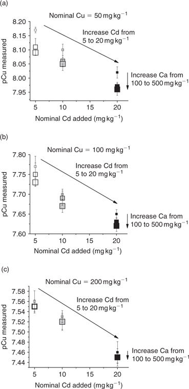
The variation of pCu as a function of the nominal Cd and Ca added is represented for the three soils in Fig. 2.
|
The competition between Cd, Ca and Cu is illustrated in these three graphs. An increase in the Cd (or Ca) treatment will increase the free Cu activities in the soil solutions. The relation is true for the three different soils as well as for the three Cu treatments. The results for each soil with each Cu treatment are not represented but the shapes of the graphs are identical. An increase of Cd additions from 5 to 20 mg kg–1 decreased the pCu to ~0.2 pCu units; this is equivalent to an increase by a factor of 1.6 in terms of activities. An increase of Ca additions from 100 to 500 mg kg–1 decreased the pCu less than 0.1 pCu units, meaning an increase by a factor of 1.25 in terms of activities. However, in contrast to studies in aqueous media where the pH can be controlled relatively carefully, the treatments of the soils with Cd and Ca decreased soil pH. This can be attributed to competition between these cations and the protons, but decreasing pH will certainly affect Cu speciation in the soil solutions. These two factors are difficult to dissociate. However, in a first qualitative approach, by comparing the relative competitive effects of Ca and Cd on the speciation of Cu, we observed that for a smaller addition of Cd, the impact on free Cu2+ was larger (Fig. 2).
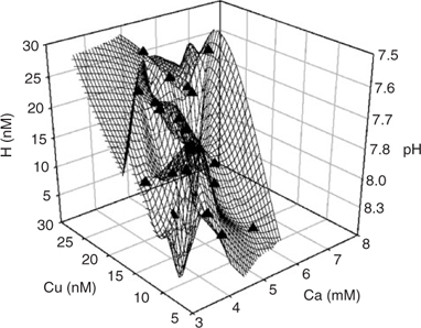
A 3-D representation of the parameters of interest (Ca, Cu and H) is found in Fig. 3. In this case, we plotted the activities of three cations instead of the negative logarithmic values because Eqn 5 was used for deducing the different parameters and this it is based on activities. Visually, we could observe a relation between the three parameters that seems to indicate an increase in the activity of a cation with increasing concentration of one or both of the other two species.
|
The shapes of the graphs are qualitatively identical for the two other soils (not shown here) and for each combination of the three cations.
Multiple regressions – a quantitative approach
To obtain the different affinity constants between the target cations and the active soil surfaces, a multiple linear regression was imposed with the pCu concentration as dependent value (response variable). Using the 27 samples of each soil independently, the regression coefficients, namely A, B, C, D and E, could be deduced. For each soil, six samples not initially integrated into the statistical determination of the regression coefficients were used to validate the linear regressions. The results for each soil are summarised independently in the three following equations. In all cases, an analysis of covariance was made and the explanatory variables (Ca2+, Cd2+, H+ and Cutot) appeared to be uncorrelated.
The relation obtained with the clay soil (Angus) is:
where R2 = 0.897, R2 adjusted = 0.871, P < 0.001.
The relation obtained with the sandy soil (Mascouche) is:
where R2 = 0.820, R2 adjusted = 0.788, P < 0.001.
The relation obtained with the sandy-organic soil (Valbo) is:
where R2 = 0.857, R2 adjusted = 0.830, P < 0.001.
In the three equations, the adjusted correlation coefficients as well as the significance values were excellent. The errors on the regression coefficients were quite high, between 11 and 50%, except for the constant parameter (E) in the Angus soil that had a 90% error value.
The relations between the pCu values predicted by these equations and the measured pCu values (not represented here) reveal that all the predicted pCu values were within a factor of 2 of the observed values and the majority of the predicted pCu values for the validation samples (not included in the determination of the regression coefficients) were also within that range. This suggests that the model is very robust for the three kinds of soils used in the experiment. However, the model can only be validated for our pH and pCu ranges and cannot be extrapolated outside these ranges.
The standardised coefficients allowed us to evaluate the relative influence of each parameter. It seems clear that the pCu concentration in soil solution is principally influenced by the total copper concentration (explains up to 50% of variance). The other components have statistically significant yet much lower contributions to explaining the pCu concentrations (explaining from 2 to 25% of variance).
In an attempt to evaluate differences among our soils, the same exercise was repeated here, but all the samples were considered in the linear regression. The resulting linear regression is represented by the following equation:
where R2 = 0.836, R2 adjusted = 0.827, P < 0.001.
The correlation coefficient and the significance value were also excellent and the errors on each regression coefficient were rather large, between 9 and 50% in this case.
The comparison of the pCu values predicted by Eqn 10 and the measured pCu (not represented here) showed that the majority of the predicted pCu were within a factor of 2 of the observed values. Moreover, the relation between the predicted and the measured pCu was excellent for two soils but presented some divergences with the clay soil (Angus), principally for the validation samples. We could explain this because clay–sand and soil organic matter (SOM) allow two different kinds of adsorption sites with different affinity constants. The determination of the different affinity constants for each soil will allow us to better evaluate this hypothesis.
As expected, the pCu concentration was principally controlled by the total copper concentration (explaining 45% of the variance) but this time the pH (explaining 30% of the variance) seemed to have a higher effect than Ca or Cd. This is in accordance with numerous papers on copper speciation in soil solution.[ 16 , 62 , 63 ] It is important to underline the significance of the pH term, given the small spread of pH values in our dataset.
The affinity constants of Ca, Cd and H were evaluated from Eqn 5 using the two approaches, for each soil individually and for all soil data combined, thus providing the individual regression coefficients A, B, C, D and E. The affinity constant for Cu was determined, in a second step, using Eqn 3 and all the samples of interest.
The resulting values are summarised in Table 2.
|
The errors on each log K value were deduced using the errors on each regression coefficient and the error propagation relations, except for log KCu for which the error came from the standard deviation of the values deduced for all the samples. The relative errors values for log K were between 2 and 9%, very encouraging for a conceptual model with a limited dataset. Moreover, the K values had the same order of magnitude as the values obtained in different TBLM studies,[ 45 , 46 ] and always in the same increasing order that is observed in BLM studies:[ 44 , 64 ] Ca << H < Cd < Cu. The affinity constants obtained for each cation in the different soils are quite similar and this suggests that it might not be necessary to differentiate the affinity constants in different soils. One possible explanation for this is that the reactivity of the soil surfaces is controlled by the heterogeneous coatings on those surfaces made up of natural organic matter, silica and metallic oxides. This coating might be similar in mineral soils of different origins and the textural class would then control the reactive surface area (measured as effective CEC) but with little influence on the selectivity of that surface. The affinity constant for Ca has the largest variability. However, the error in these values is very high owing to the error propagation and the very low affinity constant values. The affinity constants obtained with all the soils are given in Table 2. The increasing order from Ca to Cu is always observed.
Simulation treatment with MINEQL: the modelling approach
In each sample, the activities of free Cu were calculated using the chemical equilibrium software MINEQL+.[
53
] The program gives the concentration of the target species from the metal ligand stoichiometry, the protonation constant and the measured stability constants. The constant parameters used for each sample were: temperature: T = 25°C (fixed), ionic strength: I = 0.01 M (fixed),
log PCO2 = –2.5 (average between open atmosphere, log PCO2 = –3.5 and atmosphere in soil,
log PCO2 = –1.5) and the concentration of the following species (Al3+, Cd2+,
Cl–, Fe3+, K+, Mg2+, Mn2+, Na+, NO3
–, Pb2+, PO4
3–, SO4
2–, Zn2+ and active soil surface concentration). The total concentrations of the target species involved (Catot, Cdtot and Cutot) were integrated, for each sample, as the exchangeable concentrations measured by BaCl2 displacement.[
58
] The experimentally measured pH values were then integrated. Moreover, by creating a new ligand ‘Soil’ in the MINEQL+ software
(with the affinity constants for each cation expressed as:  etc.…) and a new organic ligand X (with α = [X] × KCu–X
and so, giving an arbitrary value to [X], log KCu–X
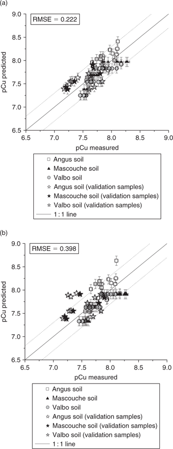
can be evaluated), we could obtain the speciation of the different solutions studied and compare the results with experimental measurements. The relation between the experimental pCu and modelled pCu is represented in Fig. 4. In the case of Fig. 4a, the affinity constants integrated in the software are the values deduced for each soil independently, and in the case of Fig. 4b, the affinity constants are the values obtained with the whole dataset.
etc.…) and a new organic ligand X (with α = [X] × KCu–X
and so, giving an arbitrary value to [X], log KCu–X
can be evaluated), we could obtain the speciation of the different solutions studied and compare the results with experimental measurements. The relation between the experimental pCu and modelled pCu is represented in Fig. 4. In the case of Fig. 4a, the affinity constants integrated in the software are the values deduced for each soil independently, and in the case of Fig. 4b, the affinity constants are the values obtained with the whole dataset.
|
The results observed in Fig. 4a are very encouraging because all the predictions are within a factor of 2 of the measured values. All the validation samples are included in this range too. The errors bars represented on the graph are: on the x-axis, the standard deviation on the three pCu measurements, and on the y-axis, the standard deviation obtained with a Monte Carlo simulation applied to the affinity constants. However, it is fastidious to use this method for integration into the MINEQL+ software; the standard deviation values of 0.1 pCu units obtained in the three samples was assumed to be representative of the other samples.
In Fig. 4b, the pCu values are predicted using MINEQL+ with the affinity constants deduced from all the soil data. This figure suggests that using an average value for the affinity constant between a cation and diverse soil surfaces is a good approximation. In fact, the majority of the pCu predictions were within a factor of 2 of the measured pCu except for some validation samples from the Angus soil (calcareous clay soil).
For the two distinct approaches, an evaluation of the model performance using the root mean square error (RMSE) was made[ 34 ]
with xi , the measured value for the data point i; xip , its predicted value; n, the number of data points; and l, the number of parameters. A small value of RMSE implies a good data fit of the model and the values obtained in Fig. 4 indicate that the model was adequate to describe the speciation of Cu in the soil solution studied. Moreover, the values of RMSE were lower than or of the same order of magnitude as other values published (0.16–0.35,[ 33 ] 0.54–1.52,[ 34 ] 0.28–0.40[ 65 ]) by various authors modelling metal speciation in soil solution with other conceptual models.
Validation of the method
For the validation of the model concept and the affinity constant values, nine other soils with different physical and chemical properties were analysed for the same parameters as the three first soils. Table 3 represents the main physicochemical properties of these soils.

|
The relation between the observed and predicted pCu following Eqns 7, 8, 9 and 10 (not represented here) reveals that each soil is better represented by one equation (Eqn 7, 8 or 9) but it is also well represented by the overall equation (Eqn 10). Moreover, the equation representing each soil seems to be in agreement with the texture of the soil. For example, the series of 7–1, 8–1 and 10–1 soils (grass cover) is better represented by the Valbo equation (sandy organic soil).
An example of the input data used for a pCu calculation is given for the Site 2B sample in the Table 4.
|
The pCu value obtained (pCu = 8.86) was then plotted v. the measured pCu value (pCu = 8.81) as well as all the other pCu values predicted by MINEQL+ with the average affinity constants v. the observed pCu (Fig. 5).
|
So, except for one soil (cor-8), all the predicted pCu were within a factor of 2 of the measured pCu. The value of RMSE (cor-8 data points are not taken into account for its calculation) is very encouraging for the validity of the model concept and for the confidence of the affinity constants for the cations of interest in the present research. The one soil presenting a rather large disparity between the predicted and the measured pCu has an acidic pH (pH = 5.2) and we attribute this divergence to the presence of Al at this pH. Under acidic soil conditions, there is a drastic increase in the solubility of Al, and Al will then occupy a significant portion of the exchangeable pool. The free Al3+ or its hydroxyl ions (Al(OH)2+ and Al(OH)2 +) will certainly compete with other cations on the active soil surfaces of the soils. The affinity constant for Al would need to be determined and integrated into the model if one is to use this approach in acidic soils. The current model seems to be robust for different kind of soils with pH > 5.5.
Conclusions
The model approach described in the present paper allows the determination of affinity constants between different cations and the active soil surfaces. The objectives were to generate a simple model within which affinity constants could be incorporated and then verify the robustness of the model in its application to several soils with different physico–chemical properties. The model works using simple soil chemistry measurements (soil pH and effective CEC) and currently only four soil ligand affinity constants. The affinity constants we obtained follow an increasing order (Ca << H < Cd < Cu) similar to that observed in the BLM and other SCMs. Moreover, the integration of these parameters in the chemical equilibrium modelling software MINEQL+ allows the speciation of the metals of interest by integrating initial characteristics of the soil (pH, CEC, total metal concentrations in soil extracts, ionic strength and CO2 pressure). The relation between the measured and predicted pCu are very encouraging when using the affinity constants for each soil or even using affinity constants obtained with the whole dataset. These results suggest that an average affinity constant value between each cation and active soil surfaces allows a reasonable evaluation of metal speciation. However, the model shows some limitations under acidic soil conditions and this is attributed to the presence of aluminium, which will compete for sorption on the active surfaces of soils and will require the determination and integration of a soil affinity constant for Al.
Acknowledgements
The authors gratefully acknowledge the support of the Natural Sciences and Engineering Research Council Metals in the Human Environment (NSERC-MITHE) research network. A complete list of sponsors is available at www.mithe-rn.org.
[1]
A. Y. Renoux ,
S. Rocheleau ,
M. Sarrazin ,
G. I. Sunahara ,
J. F. Blais ,
Assessment of a sewage sludge treatment on cadmium, copper and zinc bioavailability in barley, ryegrass and earthworms.
Environ. Pollut. 2007
, 145, 41.
| Crossref | GoogleScholarGoogle Scholar | PubMed |

[2]
F. Degryse ,
E. Smolders ,
R. Merckx ,
Labile Cd complexes increase Cd availability to plants.
Environ. Sci. Technol. 2006
, 40, 830.
| Crossref | GoogleScholarGoogle Scholar | PubMed |
[3]
J. I. Lorenzo ,
O. Nieto ,
R. Beiras ,
Effect of humic acids on speciation and toxicity of copper to Paracentrotus lividus larvae in seawater.
Aquat. Toxicol. 2002
, 58, 27.
| Crossref | GoogleScholarGoogle Scholar | PubMed |
[4]
G. J. Nierop ,
B. Jansen ,
J. A. Vrugt ,
J. M. Verstraten ,
Copper complexation by dissolved organic matter and uncertainty assessment of their stability constants.
Chemosphere 2002
, 49, 1191.
| Crossref | GoogleScholarGoogle Scholar | PubMed |
[5]
H. Ernstberger ,
W. Davison ,
H. Zhang ,
A. Tye ,
S. Young ,
Measurement and dynamic modeling of trace metal mobilization in soils using DGT and DIFS.
Environ. Sci. Technol. 2002
, 36, 349.
| Crossref | GoogleScholarGoogle Scholar | PubMed |
[6]
H. Ernstberger ,
H. Zhang ,
A. Tye ,
S. Young ,
W. Davison ,
Desorption kinetics of Cd, Zn, and Ni measured in soils by DGT.
Environ. Sci. Technol. 2005
, 39, 1591.
| Crossref | GoogleScholarGoogle Scholar | PubMed |
[7]
F. Degryse ,
E. Smolders ,
I. Oliver ,
H. Zhang ,
Relating soil solution Zn concentration to diffusive gradients in thin films measurements in contaminated soils.
Environ. Sci. Technol. 2003
, 37, 3958.
| Crossref | GoogleScholarGoogle Scholar | PubMed |
[8]
J. Rachou ,
S. Sauvé ,
W. H. Hendershot ,
Effects of pH on fluxes of cadmium in soils measured by using diffusive gradients in thin films.
Commun. Soil Sci. Plant Anal. 2004
, 35, 2655.
| Crossref | GoogleScholarGoogle Scholar |
[9]
J. Rachou ,
W. H. Hendershot ,
S. Sauvé ,
Diffusive gradients in thin films (DGT) – induced fluxes of cadmium in soils: effects of organic matter.
Commun. Soil Sci. Plant Anal. 2007
, 38, 1619.
| Crossref | GoogleScholarGoogle Scholar |
[10]
H. Zhang ,
W. Davison ,
A. M. Tye ,
N. M. J. Crout ,
S. D. Young ,
Kinetics of zinc and cadmium release in freshly contaminated soils.
Environ. Toxicol. Chem. 2006
, 25, 664.
| Crossref | GoogleScholarGoogle Scholar | PubMed |
[11]
W. Li ,
H. Zhao ,
P. R. Teasdale ,
R. John ,
F. Wang ,
Metal speciation measurement by diffusive gradients in thin films technique with different binding phases.
Anal. Chim. Acta 2005
, 533, 193.
| Crossref | GoogleScholarGoogle Scholar |
[12]
A. Avdeef ,
J. Zabronsky ,
H. H. Stuting ,
Calibration of copper ion selective electrode response to Pcu-19.
Anal. Chem. 1983
, 55, 298.
| Crossref | GoogleScholarGoogle Scholar |
[13]
S. E. Cabaniss ,
M. S. Shuman ,
Combined ion selective electrode and fluorescence quenching detection for copper–dissolved organic matter titrations.
Anal. Chem. 1986
, 58, 398.
| Crossref | GoogleScholarGoogle Scholar |
[14]
J. Gulens ,
Assessment of the research on the preparation, response and application of solid-state copper ion-selective electrodes.
Ion-Sel. Electrode R. 1987
, 9, 127.
[15]
S. Sauvé ,
M. B. McBride ,
W. H. Hendershot ,
Ion-selective electrode measurements of copper(II) activity in contaminated soils.
Arch. Environ. Contam. Toxicol. 1995
, 29, 373.
| Crossref | GoogleScholarGoogle Scholar |
[16]
S. Sauvé ,
M. B. McBride ,
W. A. Norvell ,
W. H. Hendershot ,
Copper solubility and speciation of in situ contaminated soils: effects of copper level, pH and organic matter.
Water Air Soil Pollut. 1997
, 100, 133.
| Crossref | GoogleScholarGoogle Scholar |
[17]
E. M. Logan ,
I. D. Pulford ,
G. T. Cook ,
A. B. MacKenzie ,
Complexation of Cu2+ and Pb2+ by peat and humic acid.
Eur. J. Soil Sci. 1997
, 48, 685.
| Crossref | GoogleScholarGoogle Scholar |
[18]
A. T. Lombardi ,
T. M. R. Hidalgo ,
A. A. H. Vieira ,
Copper complexing properties of dissolved organic materials exuded by the freshwater microalgae Scenedesmus acuminatus (Chlorophyceae).
Chemosphere 2005
, 60, 453.
| Crossref | GoogleScholarGoogle Scholar | PubMed |
[19]
J. Rachou ,
C. Gagnon ,
S. Sauvé ,
Use of an ion-selective electrode for free copper measurements in low salinity and low ionic strength matrices.
Environ. Chem. 2007
, 4, 90.
| Crossref | GoogleScholarGoogle Scholar |
[20]
E. P. Achterberg ,
C. Braungardt ,
Stripping voltammetry for the determination of trace metal speciation and in-situ measurements of trace metal distributions in marine waters.
Anal. Chim. Acta 1999
, 400, 381.
| Crossref | GoogleScholarGoogle Scholar |
[21]
H. P. van Leeuwen ,
S. Jansen ,
Dynamic aspects of metal speciation by competitive ligand exchange-adsorptive stripping voltammetry (CLE-AdSV).
J. Electroanal. Chem. 2005
, 579, 337.
| Crossref | GoogleScholarGoogle Scholar |
[22]
K. N. Buck ,
K. W. Bruland ,
Copper speciation in San Francisco Bay: a novel approach using multiple analytical windows.
Mar. Chem. 2005
, 96, 185.
| Crossref | GoogleScholarGoogle Scholar |
[23]
S. Meylan ,
N. Odzak ,
R. Behra ,
L. Sigg ,
Speciation of copper and zinc in natural freshwater: comparison of voltammetric measurements, diffusive gradients in thin films (DGT) and chemical equilibrium models.
Anal. Chim. Acta 2004
, 510, 91.
| Crossref | GoogleScholarGoogle Scholar |
[24]
N. Serrano ,
J. M. Diaz-Cruz ,
C. Arino ,
M. Esteban ,
Comparison of constant-current stripping chronopotentiometry and anodic stripping voltammetry in metal speciation studies using mercury drop and film electrodes.
J. Electroanal. Chem. 2003
, 560, 105.
| Crossref | GoogleScholarGoogle Scholar |
[25]
C. R. Janssen ,
D. G. Heijerick ,
K. A. C. De Schamphelaere ,
H. E. Allen ,
Environmental risk assessment of metals: tools for incorporating bioavailability.
Environ. Int. 2003
, 28, 793.
| Crossref | GoogleScholarGoogle Scholar | PubMed |
[26]
[27]
N. Semerci ,
F. Cecen ,
Importance of cadmium speciation in nitrification inhibition.
J. Hazard. Mater. 2007
, 147, 503.
| Crossref | GoogleScholarGoogle Scholar | PubMed |
[28]
J. W. Guthrie ,
N. M. Hassan ,
M. S. A. Salam ,
I. I. Fasfous ,
C. A. Murimboh ,
C. L. Murimboh ,
C. L. Chakrabarti ,
D. C. Grégoire ,
Complexation of Ni, Cu, Zn, and Cd by DOC in some metal-impacted freshwater lakes: a comparison of approaches using electrochemical determination of free-metal-ion and labile complexes and a computer speciation model, WHAM V and VI.
Anal. Chim. Acta 2005
, 528, 205.
| Crossref | GoogleScholarGoogle Scholar |
[29]
B. Cloutier-Hurteau ,
S. Sauvé ,
F. Courchesne ,
Comparing WHAM 6 and MINEQL+ 4.5 for the chemical speciation of Cu2+ in the rhizosphere of forest soils.
Environ. Sci. Technol. 2007
, 41, 8104.
| Crossref | GoogleScholarGoogle Scholar | PubMed |
[30]
C. A. M. van Gestel ,
G. Hoogerwerf ,
Influence of soil pH on the toxicity of aluminium for Eisenia andrei (Oligochaeta: Lumbricidae) in an artificial soil substrate.
Pedobiologia 2001
, 45, 385.
| Crossref | GoogleScholarGoogle Scholar |
[31]
C. Rensing ,
R. M. Maier ,
Issues underlying use of biosensors to measure metal bioavailability.
Ecotoxicol. Environ. Saf. 2003
, 56, 140.
| Crossref | GoogleScholarGoogle Scholar | PubMed |
[32]
D. J. Walker ,
R. Clemente ,
M. P. Bernal ,
Contrasting effects of manure and compost on soil pH, heavy metal availability and growth of Chenopodium album L. in a soil contaminated by pyritic mine waste.
Chemosphere 2004
, 57, 215.
| Crossref | GoogleScholarGoogle Scholar | PubMed |
[33]
J. D. MacDonald ,
W. H. Hendershot ,
Modelling trace metal partitioning in forest floors of northern soils near metal smelters.
Environ. Pollut. 2006
, 143, 228.
| Crossref | GoogleScholarGoogle Scholar | PubMed |
[34]
Y. Ge ,
D. MacDonald ,
S. Sauvé ,
W. Hendershot ,
Modeling of Cd and Pb speciation in soil solutions by WinHumicV and NICA-Donnan model.
Environ. Model. Softw. 2005
, 20, 353.
| Crossref | GoogleScholarGoogle Scholar |
[35]
S. Goldberg ,
S. J. Traina ,
Chemical modeling of anion competition on oxides using the constant capacitance model mixed-ligand approach.
Soil Sci. Soc. Am. J. 1987
, 51, 929.
[36]
X. Wen ,
Q. Du ,
H. Tang ,
Surface complexation model for the heavy metal adsorption on natural sediment.
Environ. Sci. Technol. 1998
, 32, 870.
| Crossref | GoogleScholarGoogle Scholar |
[37]
J. Choi ,
Geochemical modeling of cadmium sorption to soil as a function of soil properties.
Chemosphere 2006
, 63, 1824.
| Crossref | GoogleScholarGoogle Scholar | PubMed |
[38]
J. P. Gustafsson ,
Modeling the acid-base properties and metal complexation of humic substances with the Stockholm humic model.
J. Colloid Interface Sci. 2001
, 244, 102.
| Crossref | GoogleScholarGoogle Scholar |
[39]
M. F. Benedetti ,
W. H. Van Riemsdijk ,
L. K. Koopal ,
Humic substances considered as a heterogeneous Donnan gel phase.
Environ. Sci. Technol. 1996
, 30, 1805.
| Crossref | GoogleScholarGoogle Scholar |
[40]
P. R. Paquin ,
R. C. Santore ,
K. B. Wu ,
C. D. Kavvadas ,
D. M. Di Toro ,
The biotic ligand model: a model of the acute toxicity of metals to aquatic life.
Environ. Sci. Policy 2000
, 3, 175.
| Crossref | GoogleScholarGoogle Scholar |
[41]
W. R. Arnold ,
R. C. Santore ,
J. S. Cotsifas ,
Predicting copper toxicity in estuarine and marine waters using the biotic ligand model.
Mar. Pollut. Bull. 2005
, 50, 1634.
| Crossref | GoogleScholarGoogle Scholar | PubMed |
[42]
P. R. Paquin ,
J. W. Gorsuch ,
S. Apte ,
G. E. Batley ,
K. C. Bowles ,
P. G. C. Campbell ,
C. G. Delos ,
D. M. Di Toro ,
R. L. Dwyer ,
F. Galvez ,
R. W. Gensemer ,
G. G. Goss ,
C. Hogstrand ,
C. R. Janssen ,
J. C. McGeer ,
R. B. Naddy ,
R. C. Playle ,
R. C. Santore ,
U. Schneider ,
W. A. Stubblefield ,
C. M. Wood ,
K. B. Wu ,
The biotic ligand model: a historical overview.
Comp. Biochem. Physiol. Part C: Toxicol. Pharmacol. 2002
, 133, 3.
| Crossref | GoogleScholarGoogle Scholar |
[43]
P. M. C. Antunes ,
E. J. Berkelaar ,
D. Boyle ,
B. A. Hale ,
W. Hendershot ,
A. Voigt ,
The biotic ligand model for plants and metals: technical challenges for field application.
Environ. Toxicol. Chem. 2006
, 25, 875.
| Crossref | GoogleScholarGoogle Scholar | PubMed |
[44]
K. A. C. De Schamphelaere ,
C. R. Janssen ,
A biotic ligand model predicting acute copper toxicity for Daphnia magna: the effects of calcium, magnesium, sodium, potassium, and pH.
Environ. Sci. Technol. 2002
, 36, 48.
| Crossref | GoogleScholarGoogle Scholar | PubMed |
[45]
S. Thakali ,
H. E. Allen ,
D. M. Di Toro ,
A. A. Ponizovsky ,
C. P. Rooney ,
F. J. Zhao ,
S. P. McGrath ,
A terrestrial biotic ligand model. 1. Development and application to Cu and Ni toxicities to barley root elongation in soils.
Environ. Sci. Technol. 2006
, 40, 7085.
| Crossref | GoogleScholarGoogle Scholar | PubMed |
[46]
S. Thakali ,
H. E. Allen ,
D. M. Di Toro ,
A. A. Ponizovsky ,
C. P. Rooney ,
F. J. Zhao ,
S. P. McGrath ,
P. Criel ,
H. Van Eeckhout ,
C. R. Janssen ,
K. Oorts ,
E. Smolders ,
Terrestrial biotic ligand model. 2. Application to Ni and Cu toxicities to plants, invertebrates, and microbes in soil.
Environ. Sci. Technol. 2006
, 40, 7094.
| Crossref | GoogleScholarGoogle Scholar | PubMed |
[47]
M. Koster ,
A. de Groot ,
M. Vijver ,
W. Peijnenburg ,
Copper in the terrestrial environment: verification of a laboratory-derived terrestrial biotic ligand model to predict earthworm mortality with toxicity observed in field soils.
Soil Biol. Biochem. 2006
, 38, 1788.
| Crossref | GoogleScholarGoogle Scholar |
[48]
P. M. C. Antunes ,
B. A. Hale ,
A. C. Ryan ,
Toxicity versus accumulation for barley plants exposed to copper in the presence of metal buffers: progress towards development of a terrestrial biotic ligand model.
Environ. Toxicol. Chem. 2007
, 26, 2282.
| Crossref | GoogleScholarGoogle Scholar | PubMed |
[49]
N. T. T. M. Steenbergen ,
F. Iaccino ,
M. de Winkel ,
L. Reijnders ,
W. J. G. M. Peijnenburg ,
Development of a biotic ligand model and a regression model predicting acute copper toxicity to the earthworm Aporrectodea caliginosa.
Environ. Sci. Technol. 2005
, 39, 5694.
| Crossref | GoogleScholarGoogle Scholar | PubMed |
[50]
D. G. Heijerick ,
K. A. C. De Schamphelaere ,
C. R. Janssen ,
Biotic ligand model development predicting Zn toxicity to the alga Pseudokirchneriella subcapitata: possibilities and limitations.
Comp. Biochem. Phys. C 2002
, 133, 207.
[51]
K. A. C. De Schamphelaere ,
D. G. Heijerick ,
C. R. Janssen ,
Refinement and field validation of a Biotic Ligand Model predicting acute copper toxicity to Daphnia magna.
Comp. Biochem. Phys. C 2002
, 133, 243.
[52]
R. C. Santore ,
R. Mathew ,
P. R. Paquin ,
D. Di Toro ,
Application of the biotic ligand model to predicting zinc toxicity to rainbow trout, fathead minnow, and Daphnia magna.
Comp. Biochem. Phys. C 2002
, 133, 271.
[53]
W. D. Schecher ,
D. C. McAvoy ,
MINEQL+: a software environment for chemical equilibrium modeling.
Comput. Environ. Urban Syst. 1992
, 16, 65.
| Crossref | GoogleScholarGoogle Scholar |
[54]
[55]
L. Weng ,
E. J. M. Temminghoff ,
W. H. Van Riemsdijk ,
Contribution of individual sorbents to the control of heavy metal activity in sandy soil.
Environ. Sci. Technol. 2001
, 35, 4436.
| Crossref | GoogleScholarGoogle Scholar | PubMed |
[56]
L. A. Miller ,
K. W. Bruland ,
Competitive equilibration techniques for determining transition metal speciation in natural waters: evaluation using model data.
Anal. Chim. Acta 1997
, 343, 161.
| Crossref | GoogleScholarGoogle Scholar |
[57]
S. Sauvé ,
W. A. Norvell ,
M. McBride ,
W. Hendershot ,
Speciation and complexation of cadmium in extracted soil solutions.
Environ. Sci. Technol. 2000
, 34, 291.
| Crossref | GoogleScholarGoogle Scholar |
[58]
[59]
[60]
[61]
[62]
Y. Ge ,
P. Murray ,
W. H. Hendershot ,
Trace metal speciation and bioavailability in urban soils.
Environ. Pollut. 2000
, 107, 137.
| Crossref | GoogleScholarGoogle Scholar | PubMed |
[63]
S. Sauvé ,
A. Dumestre ,
M. McBride ,
W. Hendershot ,
Derivation of soil quality criteria using predicted chemical speciation of Pb2+ and Cu2+.
Environ. Toxicol. Chem. 1998
, 17, 1481.
| Crossref | GoogleScholarGoogle Scholar |
[64]
R. C. Playle ,
Using multiple metal-gill binding models and the toxic unit concept to help reconcile multiple-metal toxicity results.
Aquat. Toxicol. 2004
, 67, 359.
| Crossref | GoogleScholarGoogle Scholar | PubMed |
[65]
L. Weng ,
E. J. M. Temminghoff ,
S. Lofts ,
E. Tipping ,
W. H. Van Riemsdijk ,
Complexation with dissolved organic matter and solubility control of heavy metals in a sandy soil.
Environ. Sci. Technol. 2002
, 36, 4804.
| Crossref | GoogleScholarGoogle Scholar | PubMed |