

A perspective on time: loss frequencies, time scales and lifetimes
Michael J. Prather A B and Christopher D. Holmes AA Earth System Science Department, University of California–Irvine, Irvine, CA 92697-3100, USA.
B Corresponding author. Email: mprather@uci.edu
Environmental Chemistry 10(2) 73-79 https://doi.org/10.1071/EN13017
Submitted: 24 January 2013 Accepted: 9 April 2013 Published: 30 May 2013
Journal Compilation © CSIRO Publishing 2013 Open Access CC BY-NC-ND
Environmental context. The need to describe the Earth’s system or any of its components with a quantity that has units of time is ubiquitous. These quantities are used as metrics of the system to describe the response to a perturbation, the cumulative effect of an action or just the budget in terms of sources and sinks. Given a complex, non-linear system, there are many different ways to derive such quantities, and careful definitions are needed to avoid mistaken approximations while providing useful parameters describing the system.
Abstract. Diagnostic quantities involving time include loss frequency, decay times or time scales and lifetimes. For the Earth’s system or any of its components, all of these are calculated differently and have unique diagnostic properties. Local loss frequency is often assumed to be a simple, linear relationship between a species and its loss rate, but this fails in many important cases of atmospheric chemistry where reactions couple across species. Lifetimes, traditionally defined as total burden over loss rate, are mistaken for a time scale that describes the complete temporal behaviour of the system. Three examples here highlight: local loss frequencies with non-linear chemistry (tropospheric ozone); simple atmospheric chemistry with multiple reservoirs (methyl bromide) and fixed chemistry but evolving lifetimes (methyl chloroform). These are readily generalised to other biogeochemistry and Earth system models.
Additional keywords: chemical modes, eigenvalues, global warming potentials.
Introduction
The description of atmospheric chemistry and composition, or other components of the Earth’s system, using a scalar with units of time or inverse time is widespread.[1–7] These quantities are often used as metrics of the system to describe the duration or decay of a perturbation, or even the cumulative effect of an action as in ozone depletion potential or global warming potential.[8–12] There are many different ways to derive metrics of time, and they describe different properties of the system. Here we carefully define three of those metrics: loss frequency (LF) that is typically used in the continuity equation for loss of a species, time scale (TS) that can describe the e-fold of a perturbation to the system, and lifetime (LT) that is a budgetary term derived from integrated burden and loss. We demonstrate which properties of the system they describe. Three examples are taken from atmospheric chemistry and biogeochemistry, but they are readily generalised.
The confusion in deriving quantities with units of time to describe an Earth system is widespread. For example, the quantity designated ‘lifetime’ is sometimes calculated inconsistently with respect to the total burden of the species, and often used in place of the true decay time when evaluating environmental effects in assessments.[13,14] Local photochemical loss frequencies are not really system lifetimes, and are only one component of what determines the dynamical time scales of the system. A careful set of definitions and derivations is needed to ensure that we are reporting, publishing and comparing the same quantities. In cases where the chemical losses are much slower than the transport time scales that mix the atmosphere, the difference between lifetime and time scale is small (e.g. for CHF3), but for those long-lived gases with chemical feedbacks this does not hold (e.g. for N2O[15]). In the former case the steady-state lifetime for any surface emissions is very close to the e-fold time scale for decay of a perturbation. This simplification fails for short-lived species,[16–19] but the lifetime remains the correct integrating factor if one scales the pulse to the steady-state pattern. A correction from lifetime to perturbation lifetime is correctly applied when calculating the environmental effect of additional emissions, such as the global warming potentials for gases with chemical feedbacks like CH4 and N2O,[4,8,15,20,21] but the time scale of those effects cannot always be represented by a simple e-fold as in most assessments.[13,14,22,23] The use of metrics involving time is powerful, can be straightforward and follows directly from the different ways of defining them.
Definitions and derivations
The continuity equation describing the rate of change of a species (y) at a given location (x) and time (t) can be written as:
The production rate is often assumed to be independent of y and includes sources, in situ chemistry, transport and radiative terms, whereas the loss rate includes in situ chemistry, transport and other terms removing y (see Prather[1]). The loss rate is often presumed to be a linear function of y, and hence the loss frequency (LF), with units of inverse time (i.e. year–1), is calculated simply as LF = L/y. LF is the eigenvalue of a one-box, linear system.
For many important cases, such as the example of tropospheric O3 presented below, the linear form of Eqn 1 is substantially incorrect. For such non-linear systems the loss frequency may change as the system evolves, nevertheless a first-order accurate description of the system comes from the Taylor expansion of Eqn 1 about the current state (y).

This corrected loss frequency, LF = –∂([P – L](y))/∂y, is the partial derivative of the chemical terms and is evaluated at the current state (y) and for a one-box, non-linear system describes the decay (or growth) of a perturbation (Δy).
A time scale (TS) has units of time (e.g. year) and should describe the temporal behaviour of the system or perturbations to it, in the sense of an e-folding time for some component:

In this notation a negative time scale describes an unstable system. For a one-variable, one-box, constant-in-time, linear system, TS = 1/LF and Eqn 3 is the solution to Eqn 1.
Most systems described by Eqn 1, however, exhibit multiple time scales that couple chemistry and transport across the system. These times scales are the inverse eigenvalues of a coupled linear system, also called mode times,[1,20,24–27] and the temporal behaviour of a single species usually involves multiple time scales, where ∑j aj = 1.

A lifetime (LT) is an integrated quantity that characterises the overall budgets or throughput of the system (e.g. emissions, losses) and has units of time (e.g. year). It is derived from the integral species (Y ≡ ∫y, kg), production (P ≡ ∫p, kg year–1) and loss (L ≡ ∫loss = ∫LF·y, kg year–1) over the system. The instantaneous lifetime in atmospheric chemistry is defined as the integrated system-wide burden of a constituent divided by the integrated loss of that constituent (LT ≡ Y/L, year). In effect, the inverse lifetime is the weighted average of the loss frequencies (<LF>).
In general the lifetime is not a time scale of the system as defined in Eqns 3 and 4 but an amalgam of these time scales. An analogy would be the human lifetime: the time from birth to death contains a mix of times of growth, development and senescence, but one’s lifetime is an integral across these processes that cover very different types of activities. For the one-variable, one-box, constant-in-time, linear system, LT = TS = 1/LF.
Lifetimes can be defined for specific losses but always use the total burden. For example, if the total loss can be split among three processes, L = La + Lb + Lc, then the ‘a’ process lifetime, LTa ≡ Y/La, and the inverse lifetimes are additive. In general, none of these are time scales of the system.
The steady-state lifetime (LTSS) is a special case when production balances loss: i.e. dy/dt = 0 at the local scale, and P = L = YSS/LTSS on the global scale. It is special also in that this lifetime represents the cumulative environmental effects of a pulse[28]: the time integral of effects (e.g. ozone depletion, surface air quality, radiative forcing) following an emission pulse of a species exactly equals the steady-state pattern of effects from that emission pattern multiplied by the steady-state lifetime of the perturbing species for that emission pattern, assuming the perturbation and decay can be linearised. These effects generally occur over a wide range of time scales (both faster and slower) than the steady-state lifetime. This leads to the somewhat confusing result that although the system-wide Eqn 7, which is used in assessments:

does not accurately describe the decay of a perturbation Y(0), it still gives the exact integral of such a pulse and can be related to eigenvalue time scales (see Eqn 4).
In non-linear systems, the lifetime of a perturbation (Δ) to the burden (Y) can differ from the lifetime of the burden itself, i.e. LTY+Δ ≠ LTY ≠ LTΔ. The perturbation lifetime (LTΔ) describes the cumulative effect of a small pulse, and it differs from the base-state lifetime if the lifetime changes with burden. To derive LTΔ consider the losses in a perturbed system, L(Y + Δ), to be the sum of the base-state loss defined as burden over lifetime plus that from the perturbation:
where the sensitivity of lifetime to burden is s = ∂ ln(LT)/∂ ln(Y), and the feedback factor on steady-state lifetime is f = 1/(1 – s). For atmospheric CH4 the feedback factor is ~1.4; and for N2O, it is ~0.92.[4,13,29,30] The perturbation lifetime is used correctly in climate and ozone assessments as a measure of the cumulative effect of a pulse emission, but it is often mistaken for the time scale (e-fold decay) of the pulse (i.e. Eqns 7–8). Thus, if the perturbation lifetime (LTY × f) of CH4 is 12 years, then a pulse of CH4 decays with a mix of time scales both greater than and less than 12 years, but the integrated effect of such a pulse (Eqn 8) has a weighting factor of 12 years. See the example of CH3Br and ozone depletion below. The loss frequency and time scales are inherent properties of the system, but the lifetime and its variants depend on how the system is being forced with sources.
Another quantity with units of time, the age-of-air in the stratosphere[31,32] or troposphere,[33] refers to the mean age (e.g. year) of an air mass since contact with some defined location (e.g. tropopause or surface). It is an integrative quantity like lifetime, only in this case the integral is over all transport paths that air could have taken since the point of last contact to reach that location. Age-of-air is traditionally defined for conserved tracers; but a photochemical age-of-air could include chemical aging of the tracer in transit; and that is what we actually calculate when simulating for example the abundance of chloroflourocarbons (CFCs) in the stratosphere. Age-of-air, like lifetime, does not describe local frequencies nor the time scales of the system. For example, the age-of-air in the upper stratosphere and mesosphere is typically 40 % or more larger that the e-fold time scale for removal of a conserved tracer from the stratosphere.[6]
Case studies
Loss frequencies, linearisation and tropospheric O3
Tropospheric ozone (O3) provides a great example of the problems in deriving loss frequencies. The photochemistry of O3 is coupled through families of radicals (e.g. HOx, NOy), and the simplistic linear assumptions often used to calculate the loss frequency or time scales of O3 are often significantly in error. Several studies have derived eigenvalues and modes for the HOx–NOy–O3 chemistry from near surface to the mesosphere.[34–37] An example of clean-air O3 chemistry in summertime mid-latitudes at the surface is given in Table 1. Here a single 24-h day is integrated with [O3] fixed for a reference case (O3 = 30 ppb, 1 ppb = 1 nmol mol–1), and 24-h average rates are reported. Here we use upper-case P and L because this is a one-box system where y = Y and p = P. Partial derivatives with respect to O3 are calculated as finite differences with a +10 % perturbation. Initial conditions of other species are typical of an unpolluted site (see Table 1). The major production rates (P1) and loss rates (L2, L3) are large (±650 ppb day–1) and approximately cancel. By carefully adding up all rates that directly include O3 production or loss (e.g. rates L7, L8 and others), we calculate a net [P – L]O3 of –1.002 ppb day–1. Note that to achieve three-place accuracy on the net [P – L], we must calculate the main terms (P1, L2) to an accuracy of six decimal places.
|
The O3 loss frequency is often calculated as loss rate divided by abundance (Eqn 1), and in Table 1 we compare these estimates with the more accurate linearisation (Eqn 2). Defining an O3 loss frequency from reactions L2 and L3 gives a large value, LF0 = 1/(0.05 days), which is unrealistic in terms of the observed fluctuations of O3. Recognising that rate 1 (O + O2 + M = O3 + M) followed by rate 2 (O3 + hν = O + O2) does not change O3, the scientific community proposed that the O3 continuity Eqn 1 be solved for the odd-oxygen (Ox) family consisting of O3 plus both forms of atomic oxygen (ground state O(3P) and metastable O(1D)). In the stratosphere this definition of Ox reasonably describes the time scales of the Chapman ozone mechanism.[1] In the troposphere, the second largest loss rate L3 (O3 + NO = NO2 + O2) is usually followed by photolysis and reformation of Ox (NO2 + hν = NO + O), and hence NO2 might also be considered as Ox. The loss frequency defined from the three largest rates of Ox loss (L6 + L7 + L8), gives a more reasonable estimate of the time scales for O3, LF1 = 1/(10.3 days). A parallel approach based on Ox assumes that the production of NO2 from peroxy radicals (POx = P4 + P5) is fixed, independent of O3, and that the sum of the remaining O3 production and loss terms represent a loss that is linear in O3 (LOx = POx – net[P – L]O3 = LF2 × O3). For the clean-air case in Table 1, LF2 = 1/(11.0 days).
The concept of Ox is used today when calculating O3 tendencies in some chemistry transport models, but including NO2 in the Ox family adds complications in tracer transport, for example, does peroxyacetyl nitrate (PAN), which forms from and thermally decomposes to NO2 in the boundary layer, count as Ox? In general it is difficult to account for the true [P – L] of O3 (–1.00 ppb day–1) using the definition of Ox. For the example here, 18 % of the net production (+0.18 ppb day–1) occurs through small rates that are hard to identify as they depend on the ambiguous definition of Ox, particularly through the NOx reactions.
Linearisation of LOx is calculated numerically by increasing O3 from 30 to 33 ppb and gives LF3 = 0.110 day–1, which is significantly larger than LF1 = 0.097 day–1 because the abundances of HO2 and OH increase with O3. A full linearisation of [P – L]O3 (Eqn 2) gives LF4 = 0.132 day–1, a further increase in the loss frequency because the Ox production rate P4 decreases by 6 % for a 10 % increase in O3.
In summary, all of the Ox-based loss frequencies can greatly underestimate the true loss frequency for an O3 perturbation. The difference between LF2 and LF4, ~40 % in the clean boundary layer, becomes significant when we use this loss frequency to evaluate O3 as a tagged tracer, such as following the stratospheric influx of O3 to the surface[38,39] or estimating the long-range transport of pollution. In both cases the decay of the tagged O3 is underestimated. In the opposite sense, the use of tagged tracers for CO[40] can overestimate the decay rate because the added CO reduces OH abundances and thus its own loss frequency. Table 1 is only an example; accurate simulation of O3 perturbations with a chemistry transport model would require linearisation of the chemical system (tangent linear model) at each time step at each location.
From lifetimes to time scales with CH3CCl3
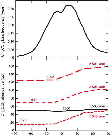
The trace gas CH3CCl3 (methyl chloroform, 1,1,1-trichloroethane) provides a case study in which the lifetime of the gas shifts as its atmospheric distribution evolves in response to changing emissions and atmospheric accumulation. Methyl chloroform is an industrially produced ozone-depleting halocarbon. Its abundance peaked in the early 1990s with a tropospheric mean of ~140 ppt (1 ppt = 1 pmol mol–1) and a North Pole to South Pole gradient of ~40 ppt due to the predominant northern sources. The latitudinal distribution from four different years (1972, 1980, 1992 and 2000) are shown in Fig. 1 (bottom). For the latter three periods these are derived from observations.[41–43] The absolute north–south gradient (ppt) is determined by the annual emissions and the rate of north–south transport. For this example we assume that it is the same from 1972 to 1992 as the mean tropospheric abundance increases. After 2000, the peak tropical loss results in a tropical depression of ~5 % in abundance that persists for the next decade as the CH3CCl3 decays at a near-uniform rate of ~0.18 year–1,[42] Over the entire period we assume that tropospheric OH remains unchanged and calculate the CH3CCl3 loss frequencies from the University of California–Irvine chemistry-transport model (CTM).[44] This annual, tropospheric, zonal mean loss frequency (Fig. 1, top) ranges from 0.01 to 0.32 year–1.
|
Combining latitudinal distribution with latitudinal loss frequency and weighting by air mass, we can calculate a lifetime against tropospheric loss for these four years. Results are given for each latitudinal profile in Fig. 1, see notes in caption. In the early years, the lifetime is largest (5.545 years) because a greater fraction of the CH3CCl3 burden is at high northern latitudes, whereas the loss frequency peaks in the tropics. As the total burden grows, a greater fraction is in the tropics and the lifetime drops (to 5.508 years in 1980 and 5.501 years in 1992). In the final stage, CH3CCl3 decays everywhere with a single e-fold, the lifetime becomes constant (5.535 years), and it is longer again because the small minimum in abundance matches the peak loss frequency in the tropics. At steady-state with the 1992 northern industrial emissions, the CH3CCl3 abundance would asymptote to ~175 ppt with a lifetime of 5.50 years (not shown). In the final phase, the lifetime (5.535 years) is also a time scale of the system, describing the decay of the longest lived chemical mode of the system, see discussion of CH3Br below. Although the differences in lifetime here are small, they serve to illustrate that even with fixed chemical loss frequencies and transport (and hence fixed time scales), the lifetime depends on the distribution of the species, which is driven by the history of emissions, as noted in the supplement of Montzka et al.[41]
Time scales coupling reservoirs with CH3Br and ozone depletion
Methyl bromide (CH3Br) presents an interesting case study of loss frequencies, time scales and lifetimes because the chemistry can be treated as fully linear but the interplay of different reservoirs (stratosphere, troposphere, ocean mixed layer) creates non-intuitive results. Methyl bromide is a naturally occurring gas with oceanic sources.[45] Its production and use in agriculture and fumigation has increased its atmospheric abundance, and the bromine radicals it releases in the stratosphere (BrY) cause ozone depletion. Formal treatment of the CH3Br system identified lifetimes and time scales that were not directly recognisable from the local loss frequencies.[46] Here, we revisit that work but collapse the 1-D chemistry diffusion problem into a three-box model with chemical model and exchange coefficients as summarised in Table 2. On the far right column of Table 2 is shown the mole fraction of CH3Br in the three reservoirs at steady-state with troposphere-only sources (scaled to 1 ppt in the troposphere). The ocean layer is equivalent to 2.9 % of the atmosphere, based on a 100-m mixed layer and the solubility of CH3Br.

|
The eigenvalue decomposition of the system with six degrees of freedom is given in Table 3. Because BrY does not feedback on CH3Br in this simplified system, there are only three CH3Br eigenvalues. These three time scales of 3.2, 0.92 and 0.018 years differ substantially from the inverse loss frequencies for CH3Br because the exchange rates between reservoirs play a key role in determining the time scales of the system. The coefficients for each time scale following a single pulse of 1 ppt CH3Br in the troposphere are given in Table 3. The abundance of CH3Br in the troposphere (trp) and stratosphere (str) follow three exponential decay curves

|
Note that trp-CH3Br decays rapidly with 0.92 years e-fold, but then ~1 % decays with the much longer 3.2 years e-fold that is tied to the decay of str-CH3Br. The str-CH3Br abundance builds initially as the CH3Br reaches the stratosphere and then decays with the single longest-lived chemical mode time for CH3Br of 3.2 years. Stratospheric BrY, effectively a proxy for ozone depletion, has more complex behaviour due to the time scale for stratosphere–troposphere exchange.
Note the str-BrY takes longer than str-CH3Br to reach its peak, and then it takes much longer to decay with a time scale of 5.6 years. These are the true time scales of the system, and not readily predicted from the loss frequencies alone.
The steady-state lifetimes derived from the budgets are given in Table 4 for three different cases with tropospheric CH3Br abundances of 10 ppt: (a) a hypothetical, troposphere-only source giving an ocean saturation level of 46 % (i.e., 4.6 ppt); (b) a hypothetical, ocean-only source giving an ocean saturation level of 177 % and (c) a mix of both sources to yield a net neutral ocean saturation of 100 %. During the peak of anthropogenic emissions in the 1990s, ocean saturation was about 85 %,[45,47] and following mitigation the abundance dropped to ~8 ppt with average ocean saturation of 100 %.[48] Note that this drop of 20 % in CH3Br tropospheric abundance requires reduction of more than 50 % in tropospheric emissions. The steady-state lifetime, 1.03 years in case A and 0.50 in case B, is straightforward. In case C the combination gives an intermediate lifetime of 0.70 years. Thus we have a clear and obvious case where the lifetime depends on the source.

|
The steady-state lifetime and pattern for a tropospheric source are important numbers in that they describe exactly the integral of exposure (e.g. ppt-year) following a single tropospheric pulse.[1,28] First, take a 1-ppt tropospheric pulse (i.e. 0.872 ppt-atm) and distribute the same burden in the steady-state pattern. This gives 0.910 ppt of CH3Br in the troposphere (with the remainder in the stratosphere and ocean) and 0.404 ppt BrY in the stratosphere. Multiplying each of these by the steady-state lifetime for tropospheric sources, 1.029 years, we get 0.936 ppt-year for trp-CH3Br and 0.416 ppt-year for str-BrY, which is exactly (with enough decimal places) the integral from zero to infinity of Eqns 11 and 13 respectively. It is important to note that the ozone depletion persists for more than 5 years although the lifetime of the CH3Br source is only ~1 year. Thus the CH3Br lifetime is the correct integrating factor for effects following the release but it fails to describe the time scales of those effects.
Conclusions
Loss frequency is often used as a simple scaling factor, relating the local loss rate of a species to its abundance. In general with coupled, multi-species systems, the simple linear scaling fails, but an effective loss frequency can be calculated for a perturbation to a species with a linearisation of the system (e.g. tropospheric O3). Lifetimes, which are defined in terms of integrated budgets, depend on the method of external forcing. The lifetime of a trace gas can change even when the chemical reactivity of the atmosphere is unchanged (e.g. CH3CCl3). For a perturbation forced by a specific emission pattern, the product of the steady-state pattern and the lifetime are an exact integral of a pulse of that emission, including any consequent environmental effects[28] (e.g. CH3Br and O3 depletion). This method of defining lifetime works even for trace gases with known chemical feedbacks or indirect effects such as N2O, CH4, CO and NOx as long as one uses the perturbation lifetime.[8,13,49,50] Even for relatively simple systems, time scales reflect the multitude of degrees of freedom (e.g. CH3Br); however, proper diagnosis even in 3-D models can identify the correct response to perturbations.[5,30,51] The often-made simplifying assumption – that these three metrics are the same – may be appealing if one is sure that the errors are small, but the lack of rigor may propagate to systems where much larger, unrecognised errors will occur.
Acknowledgements
This research was supported by the NASA Modelling, Analysis, and Prediction Program (NNX09AJ47G), the Office of Science (BER) of the US Department of Energy (DE-SC0007021), and the Kavli Chair in Earth System Science.
References
[1] M. J. Prather, Lifetimes and time scales in atmospheric chemistry. Philos. Trans. Roy. Soc. A 2007, 365, 1705.| Lifetimes and time scales in atmospheric chemistry.Crossref | GoogleScholarGoogle Scholar | 1:CAS:528:DC%2BD2sXot1Kks70%3D&md5=e54541971e6e3fb921ce4f9c5b6d6c9eCAS |
[2] B. Bolin, H. Rodhe, Note on concepts of age distribution and transit-time in natural reservoirs. Tellus 1973, 25, 58.
| Note on concepts of age distribution and transit-time in natural reservoirs.Crossref | GoogleScholarGoogle Scholar |
[3] C. E. Junge, Residence time and variability of tropospheric trace gases. Tellus 1974, 26, 477.
| Residence time and variability of tropospheric trace gases.Crossref | GoogleScholarGoogle Scholar | 1:CAS:528:DyaE2MXjtlGluw%3D%3D&md5=c540c3c28bab4bc3ba6e8c874ff5606dCAS |
[4] M. J. Prather, Lifetimes and eigenstates in atmospheric chemistry. Geophys. Res. Lett. 1994, 21, 801.
| Lifetimes and eigenstates in atmospheric chemistry.Crossref | GoogleScholarGoogle Scholar | 1:CAS:528:DyaK2cXmtV2mtbY%3D&md5=d878f31a92ef51b0af42290985a8f81eCAS |
[5] R. G. Derwent, W. J. Collins, C. E. Johnson, D. S. Stevenson, Transient behaviour of tropospheric ozone precursors in a global 3-D CTM and their indirect greenhouse effects. Clim. Change 2001, 49, 463.
| Transient behaviour of tropospheric ozone precursors in a global 3-D CTM and their indirect greenhouse effects.Crossref | GoogleScholarGoogle Scholar | 1:CAS:528:DC%2BD3MXks1KqsrY%3D&md5=f7a73ce9d33fadc4726e8de8cf62370dCAS |
[6] D. H. Ehhalt, F. Rohrer, S. Schauffler, M. J. Prather, On the decay of stratospheric pollutants: diagnosing the longest-lived eigenmode. J. Geophys. Res. – Atmos. 2004, 109, D08102.
| On the decay of stratospheric pollutants: diagnosing the longest-lived eigenmode.Crossref | GoogleScholarGoogle Scholar |
[7] B. C. O’Neill, S. R. Gaffin, F. N. Tubiello, M. Oppenheimer, Reservoir timescales for anthropogenic CO2 in the atmosphere. Tellus B Chem. Phys. Meterol. 1994, 46, 378.
| Reservoir timescales for anthropogenic CO2 in the atmosphere.Crossref | GoogleScholarGoogle Scholar |
[8] J. S. Fuglestvedt, I. S. A. Isaksen, W. C. Wang, Estimates of indirect global warming potentials for CH4, CO and NOx. Clim. Change 1996, 34, 405.
| Estimates of indirect global warming potentials for CH4, CO and NOx.Crossref | GoogleScholarGoogle Scholar | 1:CAS:528:DyaK2sXoslGktQ%3D%3D&md5=c5a0445d931ec46f179bd3c41a77a1e2CAS |
[9] J. S. Daniel, S. Solomon, D. L. Albritton, On the evaluation of halocarbon radiative forcing and global warming potentials. J. Geophys. Res. – Atmos. 1995, 100, 1271.
| On the evaluation of halocarbon radiative forcing and global warming potentials.Crossref | GoogleScholarGoogle Scholar | 1:CAS:528:DyaK2MXktlaqs74%3D&md5=7521ec50cf5e49d1ff87f2189f9826caCAS |
[10] S. Solomon, D. L. Albritton, Time-dependent ozone depletion potentials for short-term and long-term forecasts. Nature 1992, 357, 33.
| Time-dependent ozone depletion potentials for short-term and long-term forecasts.Crossref | GoogleScholarGoogle Scholar | 1:CAS:528:DyaK38XktFemtbg%3D&md5=a4c0ddd6ec41eb347a4b6ffda5c8985aCAS |
[11] D. J. Wuebbles, Weighing functions for ozone depletion and greenhouse-gas effects on climate. Annu. Rev. Energy Environ. 1995, 20, 45.
| Weighing functions for ozone depletion and greenhouse-gas effects on climate.Crossref | GoogleScholarGoogle Scholar |
[12] D. L. Albritton, R. G. Derwent, I. S. A. Isaksen, M. Lal, D. J. Wuebbles, Trace gas radiative forcing indices, in Climate Change 1994, Intergovernmental Panel on Climate Change (Eds J. T. Houghton, L. G. Meira-Filho, J. Bruce, H. Lee, B. A. Callander, E. Haites, N. Harris, K. Maskell) 1995, pp. 202–231 (Cambridge University Press: Cambridge UK).
[13] P. Forster, V. Ramaswamy, P. Artaxo, T. Berntsen, R. Betts, D. W. Fahey, J. Haywood, J. Lean, D. C. Lowe, G. Myhre, J. Nganga, R. Prinn, G. Raga, M. Schulz, R. Van Dorland, Changes in atmospheric constituents and in radiative forcing in Climate Change 2007: The Physical Science Basis Fourth Assessment Report of the Intergovernmental Panel on Climate Change (Eds S. Solomon, D. Qin, M. Manning) 2007, pp. 129–234 (Cambridge University Press: Cambridge UK).
[14] Scientific Assessment of Ozone Depletion: 2010 2010 (World Meteorological Organization: Geneva, Switzerland).
[15] M. J. Prather, J. Hsu, Coupling of nitrous oxide and methane by global atmospheric chemistry. Science 2010, 330, 952.
| Coupling of nitrous oxide and methane by global atmospheric chemistry.Crossref | GoogleScholarGoogle Scholar | 1:CAS:528:DC%2BC3cXhtl2isbvK&md5=6d926a53e8bb247efbd24fb509c5b3e0CAS | 21071666PubMed |
[16] S. C. Olsen, B. J. Hannegan, X. Zhu, M. J. Prather, Evaluating ozone depletion from very short-lived halocarbons. Geophys. Res. Lett. 2000, 27, 1475.
| Evaluating ozone depletion from very short-lived halocarbons.Crossref | GoogleScholarGoogle Scholar | 1:CAS:528:DC%2BD3cXjvVGhs7s%3D&md5=a3094db51e07dc953c317694718da419CAS |
[17] C. H. Bridgeman, J. A. Pyle, D. E. Shallcross, A three-dimensional model calculation of the ozone depletion potential of 1-bromopropane (1-C3H7Br). J. Geophys. Res. – Atmos. 2000, 105, 26 493.
| A three-dimensional model calculation of the ozone depletion potential of 1-bromopropane (1-C3H7Br).Crossref | GoogleScholarGoogle Scholar | 1:CAS:528:DC%2BD3cXovVGrs7g%3D&md5=15aedc51c7dd190b8a134beb353911d8CAS |
[18] D. J. Wuebbles, K. O. Patten, M. T. Johnson, R. Kotamarthi, New methodology for Ozone depletion potentials of short-lived compounds: n-propyl bromide as an example. J. Geophys. Res. – Atmos. 2001, 106, 14 551.
| New methodology for Ozone depletion potentials of short-lived compounds: n-propyl bromide as an example.Crossref | GoogleScholarGoogle Scholar | 1:CAS:528:DC%2BD3MXlvVGqtrk%3D&md5=7cd5ee31c111ef7ff7c78d1b2217c81aCAS |
[19] A. Mellouki, R. K. Talukdar, A. M. Schmoltner, T. Gierczak, M. J. Mills, S. Solomon, A. R. Ravishankara, Atmospheric lifetimes and ozone depletion potentials of methyl-bromide (CH3Br) and dibromomethane (CH2Br2). Geophys. Res. Lett. 1992, 19, 2059.
| Atmospheric lifetimes and ozone depletion potentials of methyl-bromide (CH3Br) and dibromomethane (CH2Br2).Crossref | GoogleScholarGoogle Scholar | 1:CAS:528:DyaK3sXitFKqsrc%3D&md5=607c37d8ece6a706919670a32571baf1CAS |
[20] M. J. Prather, Time scales in atmospheric chemistry: theory, GWPs for CH4 and CO, and runaway growth. Geophys. Res. Lett. 1996, 23, 2597.
| Time scales in atmospheric chemistry: theory, GWPs for CH4 and CO, and runaway growth.Crossref | GoogleScholarGoogle Scholar | 1:CAS:528:DyaK28XmsFWis74%3D&md5=01fec7d1a15bbe8a3a6ab26b29636f77CAS |
[21] F. Raes, H. Liao, W. T. Chen, J. H. Seinfeld, Atmospheric chemistry–climate feedbacks. J. Geophys. Res. – Atmos. 2010, 115, D12121.
| Atmospheric chemistry–climate feedbacks.Crossref | GoogleScholarGoogle Scholar |
[22] M. J. Prather, D. Ehhalt, F. Dentener, R. Derwent, E. Dlugokencky, E. Holland, I. Isaksen, J. Katime, V. Kirchhoff, P. Matson, P. Midgley, M. Wang, Atmospheric chemistry and greenhouse gases, in Climate Change 2001: The Scientific Basis Third Assessment Report of the Intergovernmental Panel on Climate Change (Eds J. T. Houghton, Y. Ding, D. J. Griggs) 2001, pp. 239–287 (Cambridge University Press: Cambridge UK).
[23] Scientific Assessment of Ozone Depletion: 2006 2006 (World Meteorological Organization: Geneva, Switzerland).
[24] M. R. Manning, Characteristic modes of isotopic variations in atmospheric chemistry. Geophys. Res. Lett. 1999, 26, 1263.
| Characteristic modes of isotopic variations in atmospheric chemistry.Crossref | GoogleScholarGoogle Scholar | 1:CAS:528:DyaK1MXjslCltLw%3D&md5=a7da11fb08006511a805b98d7b387b8dCAS |
[25] B. F. Farrell, P. J. Ioannou, Perturbation dynamics in atmospheric chemistry. J. Geophys. Res. – Atmos. 2000, 105, 9303.
| Perturbation dynamics in atmospheric chemistry.Crossref | GoogleScholarGoogle Scholar | 1:CAS:528:DC%2BD3cXjtFSgtLs%3D&md5=7fd92b60f5b19c93e54bff60778db7c6CAS |
[26] K. R. Lassey, D. C. Lowe, M. R. Manning, The trend in atmospheric methane δ13C implications for isotopic constraints on the global methane budget. Global Biogeochem. Cycles 2000, 14, 41.
| The trend in atmospheric methane δ13C implications for isotopic constraints on the global methane budget.Crossref | GoogleScholarGoogle Scholar | 1:CAS:528:DC%2BD3cXhvVGnu78%3D&md5=63026e8f6743a144148d971cc70b4df8CAS |
[27] J. Y. Xu, A. K. Smith, Evaluation of processes that affect the photochemical timescale of the sodium layer. J. Atmos. Sol. Terr. Phys. 2005, 67, 1216.
| Evaluation of processes that affect the photochemical timescale of the sodium layer.Crossref | GoogleScholarGoogle Scholar | 1:CAS:528:DC%2BD2MXpslahtLo%3D&md5=d2eff39c8c3084b0493e7ff85d2583f7CAS |
[28] M. J. Prather, Lifetimes of atmospheric species: integrating environmental impacts. Geophys. Res. Lett. 2002, 29, 2063.
| Lifetimes of atmospheric species: integrating environmental impacts.Crossref | GoogleScholarGoogle Scholar |
[29] M. J. Prather, Time scales in atmospheric chemistry: coupled perturbations to N2O, NOy, and O3. Science 1998, 279, 1339.
| Time scales in atmospheric chemistry: coupled perturbations to N2O, NOy, and O3.Crossref | GoogleScholarGoogle Scholar | 1:CAS:528:DyaK1cXhtleqsbs%3D&md5=01309eed97c3d33d7ff3532050a2fc67CAS | 9478891PubMed |
[30] J. Hsu, M. J. Prather, Global long-lived chemical modes excited in a 3-D chemistry transport model: stratospheric N2O, NOy, O3 and CH4 chemistry. Geophys. Res. Lett. 2010, 37, L07805.
| Global long-lived chemical modes excited in a 3-D chemistry transport model: stratospheric N2O, NOy, O3 and CH4 chemistry.Crossref | GoogleScholarGoogle Scholar |
[31] T. M. Hall, D. W. Waugh, Stratospheric residence time and its relationship to mean age. J. Geophys. Res. 2000, 105, 6773.
| Stratospheric residence time and its relationship to mean age.Crossref | GoogleScholarGoogle Scholar | 1:CAS:528:DC%2BD3cXisVakurs%3D&md5=745002d9aca910894e79fb769758dd45CAS |
[32] T. M. Hall, R. A. Plumb, Age as a diagnostic of stratospheric transport. J. Geophys. Res. – Atmos. 1994, 99, 1059.
| Age as a diagnostic of stratospheric transport.Crossref | GoogleScholarGoogle Scholar | 1:CAS:528:DyaK2cXltFKgt7s%3D&md5=848a27cca54c090028d1304f32c74a7bCAS |
[33] M. J. Prather, X. Zhu, Q. Tang, J. N. Hsu, J. L. Neu, An atmospheric chemist in search of the tropopause. J. Geophys. Res. – Atmos. 2011, 116, D04306.
| An atmospheric chemist in search of the tropopause.Crossref | GoogleScholarGoogle Scholar |
[34] L. Jaeglé, D. J. Jacob, W. H. Brune, P. O. Wennberg, Chemistry of HOx radicals in the upper troposphere. Atmos. Environ. 2001, 35, 469.
| Chemistry of HOx radicals in the upper troposphere.Crossref | GoogleScholarGoogle Scholar |
[35] G. Sonnemann, B. Fichtelmann, Subharmonics, cascades of period doubling, and chaotic behavior of photochemistry of the mesopause region. J. Geophys. Res. – Atmos. 1997, 102, 1193.
| Subharmonics, cascades of period doubling, and chaotic behavior of photochemistry of the mesopause region.Crossref | GoogleScholarGoogle Scholar | 1:CAS:528:DyaK2sXhtFGlsr4%3D&md5=c1ab86e3ca540daa77d8debea67a6f99CAS |
[36] J. G. Esler, An integrated approach to mixing sensitivities in tropospheric chemistry: a basis for the parameterization of subgrid-scale emissions for chemistry transport models. J. Geophys. Res. – Atmos. 2003, 108, 4632.
| An integrated approach to mixing sensitivities in tropospheric chemistry: a basis for the parameterization of subgrid-scale emissions for chemistry transport models.Crossref | GoogleScholarGoogle Scholar |
[37] N. Bell, D. E. Heard, M. J. Pilling, A. S. Tomlin, Atmospheric lifetime as a probe of radical chemistry in the boundary layer. Atmos. Environ. 2003, 37, 2193.
| Atmospheric lifetime as a probe of radical chemistry in the boundary layer.Crossref | GoogleScholarGoogle Scholar | 1:CAS:528:DC%2BD3sXivVCrs70%3D&md5=535f0a90d234a239ef37cee2b24ce78aCAS |
[38] O. Wild, M. J. Prather, H. Akimoto, J. K. Sundet, I. S. A. Isaksen, J. H. Crawford, D. D. Davis, M. A. Avery, Y. Kondo, G. W. Sachse, S. T. Sandholm, Chemical transport model ozone simulations for spring 2001 over the western Pacific: regional ozone production and its global impacts. J. Geophys. Res. – Atmos. 2004, 109, D15S02.
[39] V. Grewe, The origin of ozone. Atmos. Chem. Phys. 2006, 6, 1495.
| The origin of ozone.Crossref | GoogleScholarGoogle Scholar | 1:CAS:528:DC%2BD28Xot1Ohtbs%3D&md5=b6dc464664bbcef37a9160254d5d1e35CAS |
[40] J. F. Lamarque, P. G. Hess, Model analysis of the temporal and geographical origin of the CO distribution during the TOPSE campaign. J. Geophys. Res. – Atmos. 2003, 108, 8354.
| Model analysis of the temporal and geographical origin of the CO distribution during the TOPSE campaign.Crossref | GoogleScholarGoogle Scholar |
[41] S. A. Montzka, C. M. Spivakovsky, J. H. Butler, J. W. Elkins, L. T. Lock, D. J. Mondeel, New observational constraints for atmospheric hydroxyl on global and hemispheric scales. Science 2000, 288, 500.
| New observational constraints for atmospheric hydroxyl on global and hemispheric scales.Crossref | GoogleScholarGoogle Scholar | 1:CAS:528:DC%2BD3cXivVKhur0%3D&md5=71157fb72dc600940c4d977880d2fa6eCAS | 10775106PubMed |
[42] S. A. Montzka, M. Krol, E. Dlugokencky, B. Hall, P. Jockel, J. Lelieveld, Small interannual variability of global atmospheric hydroxyl. Science 2011, 331, 67.
| Small interannual variability of global atmospheric hydroxyl.Crossref | GoogleScholarGoogle Scholar | 1:CAS:528:DC%2BC3MXpslan&md5=cade4d8831c263e6f1b018938ee1a993CAS | 21212353PubMed |
[43] M. Rigby, R. G. Prinn, S. O’Doherty, S. A. Montzka, A. McCulloch, C. M. Harth, J. Mühle, P. K. Salameh, R. F. Weiss, D. Young, P. G. Simmonds, B. D. Hall, G. S. Dutton, D. Nance, D. J. Mondeel, J. W. Elkins, P. B. Krummel, L. P. Steele, P. J. Fraser, Re-evaluation of the lifetimes of the major CFCs and CH3CCl3 using atmospheric trends. Atmos. Chem. Phys. Discuss. 2012, 12, 24 469.
| Re-evaluation of the lifetimes of the major CFCs and CH3CCl3 using atmospheric trends.Crossref | GoogleScholarGoogle Scholar |
[44] C. D. Holmes, M. J. Prather, O. A. Sovde, G. Myhre, Future methane, hydroxyl, and their uncertainties: key climate and emission parameters for future predictions. Atmos. Chem. Phys. 2013, 13, 285.
| Future methane, hydroxyl, and their uncertainties: key climate and emission parameters for future predictions.Crossref | GoogleScholarGoogle Scholar |
[45] S. A. Yvon-Lewis, J. H. Butler, The potential effect of oceanic biological degradation on the lifetime of atmospheric CH3Br. Geophys. Res. Lett. 1997, 24, 1227.
| The potential effect of oceanic biological degradation on the lifetime of atmospheric CH3Br.Crossref | GoogleScholarGoogle Scholar | 1:CAS:528:DyaK2sXjvFegsb8%3D&md5=91adeffb88bd3c4744af192f80233e72CAS |
[46] M. J. Prather, Timescales in atmospheric chemistry: CH3Br, the ocean, and ozone depletion potentials. Global Biogeochem. Cycles 1997, 11, 393.
| Timescales in atmospheric chemistry: CH3Br, the ocean, and ozone depletion potentials.Crossref | GoogleScholarGoogle Scholar | 1:CAS:528:DyaK2sXls1Krurs%3D&md5=f9b84c83141f468ca66174092c821186CAS |
[47] J. H. Butler, Scientific uncertainties in the budget of atmospheric methyl bromide. Atmos. Environ. 1996, 30, R1.
[48] L. Hu, S. A. Yvon-Lewis, Y. Liu, T. S. Bianchi, The ocean in near equilibrium with atmospheric methyl bromide. Global Biogeochem. Cycles 2012, 24, 1227.
[49] J. S. Daniel, S. Solomon, On the climate forcing of carbon monoxide. J. Geophys. Res. – Atmos. 1998, 103, 13 249.
| On the climate forcing of carbon monoxide.Crossref | GoogleScholarGoogle Scholar | 1:CAS:528:DyaK1cXktleksLg%3D&md5=c9a617d976dc2ce49c591bd97856437eCAS |
[50] K. P. Shine, T. K. Berntsen, J. S. Fuglestvedt, R. Sausen, Scientific issues in the design of metrics for inclusion of oxides of nitrogen in global climate agreements. Proc. Natl. Acad. Sci. USA 2005, 102, 15 768.
| Scientific issues in the design of metrics for inclusion of oxides of nitrogen in global climate agreements.Crossref | GoogleScholarGoogle Scholar | 1:CAS:528:DC%2BD2MXht1Wru7jL&md5=3d3f19776c7b197d91d9a4bf6a86d2beCAS |
[51] O. Wild, M. J. Prather, Excitation of the primary tropospheric chemical mode in a global three-dimensional model. J. Geophys. Res. – Atmos. 2000, 105, 24 647.
| Excitation of the primary tropospheric chemical mode in a global three-dimensional model.Crossref | GoogleScholarGoogle Scholar | 1:CAS:528:DC%2BD3cXotVyrtbk%3D&md5=23db02003de0c0627ea5550925578685CAS |
[52] C. D. Holmes, M. J. Prather, A. O. Søvde, G. Myhre, Future methane, hydroxyl, and their uncertainties: key climate and emission parameters for future predictions. Atmos. Chem. Phys. Discuss. 2012, 12, 20 931.
| Future methane, hydroxyl, and their uncertainties: key climate and emission parameters for future predictions.Crossref | GoogleScholarGoogle Scholar |
[53] M. J. Prather, C. D. Holmes, J. Hsu, Reactive greenhouse gas scenarios: systematic exploration of uncertainties and the role of atmospheric chemistry. Geophys. Res. Lett. 2012, 39, L09803.
| Reactive greenhouse gas scenarios: systematic exploration of uncertainties and the role of atmospheric chemistry.Crossref | GoogleScholarGoogle Scholar |