

Application of the Groenevelt–Grant soil water retention model to predict the hydraulic conductivity
C. D. Grant A D , P. H. Groenevelt B and N. I. Robinson CA School of Agriculture, Food and Wine, University of Adelaide, Waite Campus, DX650-614, PMB-1 Glen Osmond, SA 5064, Australia.
B School of Environmental Sciences, University of Guelph, Guelph, ON N1G 2W1, Canada.
C School of Chemistry, Physics and Earth Sciences, Flinders University, GPO Box 2100, Adelaide, SA 5001, Australia.
D Corresponding author. Email: cameron.grant@adelaide.edu.au
Australian Journal of Soil Research 48(5) 447-458 https://doi.org/10.1071/SR09198
Submitted: 3 November 2009 Accepted: 24 March 2010 Published: 6 August 2010
Abstract
We outline several formulations of the Groenevelt–Grant water retention model of 2004 to show how it can be anchored at different points. The model is highly flexible and easy to perform multiple differentiations and integrations on. Among many possible formulations of the model we choose one anchored solely at the saturated water content, θs, to facilitate comparison with the van Genuchten model of 1980 and to obtain a hydraulic conductivity function through analytical integration:
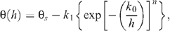
where, k0, k1, and n are fitting parameters. We divided this formulation by θs to obtain the relative water content, θr(h), and inverted the function to produce a form required for integration, namely:
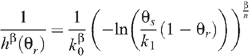
in which the parameter β is introduced to accommodate both the ‘Burdine’ and ‘Mualem’ models. The integrals are identified as incomplete gamma functions and are distinctly different from the incomplete beta functions embodied in the van Genuchten–Mualem models.
Rijtema’s data from 1969 for 20 Dutch soils are used to demonstrate the procedures involved. The water retention curves produced by our Groenevelt–Grant model are virtually indistinguishable from those produced by the van Genuchten model. Relative hydraulic conductivities produced by our Mualem and Burdine models produced closer estimates of Rijtema’s measured values than those produced by the van Genuchten–Mualem model for 19 of his 20 soils. This work provides an alternative to the widely used van Genuchten–Mualem approach and represents a preamble for the, as yet unsatisfactory, treatment of the tortuosity component of the unsaturated hydraulic conductivity function.
Additional keyword: incomplete gamma function.
Acknowledgment and historical note
We thank Dr Robert S. Murray, School of Earth & Environmental Sciences at the University of Adelaide, who generously covered the senior author’s lecture commitments during March and April 2006 while the co-authors of this paper were in Adelaide. We also thank the University of Adelaide for allowing the senior author to take study leave during 2007 and 2008 to continue this work in Guelph. In 1963, the second author started his career at the Instituut voor Cultuurtechniek en Waterhuishouding (ICW), the home base of Dr Peter E. Rijtema (1929–2006). There, over a period of four decades, Rijtema carried out original and visionary research and produced high-quality soil-water data, a set of which we have used in the present paper. Finally, we acknowledge helpful suggestions from reviewers of this paper on statistics to evaluate the model.
Assouline S
(2001) A model for soil relative hydraulic conductivity based on the water retention characteristic curve. Water Resources Research 37, 265–271. (cf. Assouline S 2004. Correction to ‘A model for soil relative hydraulic conductivity based on the water retention characteristic curve’. Water Resources Research 40, W02901.
| Crossref | GoogleScholarGoogle Scholar |
one form of the general model (Eqn 4) based on one anchor point only, viz. the point of saturation (θr = 1, hs = 0). There are situations, however, in which one may wish to use 2 or even 3 points for ‘anchoring’. If one considers 2 ‘anchor points’ for example, the fitting parameter k1 can be eliminated from the general model, leaving the 2 remaining parameters for optimisation. If one has confidence in the measured water content at the wilting point (θw), a good set of anchor points could then be the ‘permanent wilting point’ and the ‘point of saturation’, which produces the form:

Now by anchoring the model at the ‘point of saturation’ (θs, hs = 0 m), the wilting point (θw, hw = 150 m), as well as a third point, say the ‘oven-dry point’ (θod = 0, hod = 104.9 m), one can eliminate k0 by substituting the coordinates for the ‘oven dry point’ into Eqn 4 and re-arranging to obtain:

The k0n from Eqn A2 can then be substituted into an equation similar to Eqn A1 with the point of saturation replaced by the oven-dry point as the second anchor. This yields:
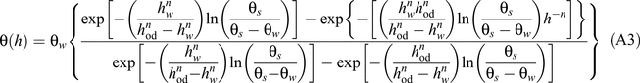
Equation A3 contains the 3 anchor points and the last remaining parameter, n.
Finally, by introducing the ‘point of irrigation’ as a fourth anchor point (e.g. the point (θir, hir,) at which irrigation is conventionally started), one may write a relation similar to Eqn A2 with the coordinates of the ‘permanent wilting point’ replaced by those of:

Combining Eqns A2 and A4 produces:
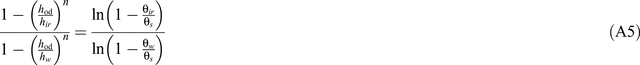
from which the parameter n can be solved numerically. This allows k0 to be solved from Eqn A2 or A4 and k1 to be solved from Eqn 5.