

Review of soil erosion modelling involving water with field applications
C. W. Rose A * and A. Haddadchi B *
A
B
Handling Editor: Stephen Anderson
Abstract
The literature associated with the topic of soil erosion processes is so vast that coverage must be restricted in some way. The major restriction adopted includes a focus on physically-based soil erosion modelling and its application in field studies including gully formation and sediment control methods. The choice of topics has also been biased towards those in which the authors have had some involvement, ensuring some emphasis on erosion studies in Australia and Southeast Asia.
Keywords: deposition, erosion mitigation strategies, field applications, gully erosion, physically-based models, sediment transport, soil conservation, soil erosion modelling.
Introduction
Viewed over geological time scales, the origin of that great variety of material we describe as ‘soil’ is the outcome of many interacting factors including physical, chemical and biological processes of many types. One such process, commonly dominantly physical in nature, but very varied in process terms, is referred to as ‘erosion’. Erosion is one of the very many naturally occurring processes involved in the creation or modification of soil and soil profiles, but too often accelerated by human activity.
Examples of the broad range of erosion processes include the glacial shearing of rock material, mass movement under gravity of whole soil volumes, the dynamic effects of impacting rainfall, overland flowing water and shearing winds. However ubiquitous, the term ‘soil erosion’ is commonly used in the particular context where such processes are perceived as damaging to the universal productive and life-sustaining role that soils fulfil, and where human activity plays a role in such degradation in landscapes or soil quality.
Increasing world population and its associated requirement for food, habitation and consumer products has resulted in many environmentally destructive or polluting activities. One consequence is that soil erosion and soil formation have become seriously out of balance (Pimentel et al. 1995). In addition to losing topsoil due to erosion, soil quality is generally degraded, which is of great concern globally, especially due to its direct effects on crop production (FAO 2019).
Soils provide the basis for most food eaten by humans. Soil is a potentially renewable resource, but retaining such potential depends on the manner in which this resource is managed. The productive potential of soil can be degraded by those forms of human land use that involve substantial soil exposure by any means, such as agricultural clean tillage and de-forestation. Accelerated soil erosion is now not only of significant concern to most societies due to its effect in reducing food production, but this concern is further stimulated by broader environmental/ethical perceptions of a responsibility to ‘care for country’, a term so enriched in meaning by aboriginal Australian conceptions. Pollution of waterways and oceans by nutrients and other chemicals is also a major concern commonly linked to soil erosion and sediment transport. Handelsman (2021) makes a compelling, well-informed case for the serious challenge to food security associated with present levels of soil erosion.
Evidence has also accumulated that the effects of a warming world climate, due to emissions of long-wave absorbing and emitting gases, amplifies climatic extremes, which can result in accelerated rates of soil erosion, therefore degrading productive soils at an increasing rate.
One response to such observed and potentially increasing threats has been to seek a better understanding of the suite of soil erosion related processes with the general aim of seeking to control them at sustainable levels by exploring better land management practices and policies. An increasing call has been made on physical theory to provide a conceptual framework for the interpretation of experimental data obtained in soil erosion investigations. This document seeks to provide a review of some of the important aspects of that endeavour, though focussed on the range of situations where rainfall and its associated or collected runoff processes are the erosive agents involved. Particular attention will be given to the role of physically-based models of the variety of erosion processes in agricultural and, to a lesser extent, riverine contexts.
As agricultural chemicals and biological pathogens bind preferentially to the finer clay and silt size fractions of soil, the ability of models to describe the size distribution of transported sediment will also receive special attention. This issue is also of consequence in describing sediment transport in riverine systems (Haddadchi and Rose 2022).
It may be noted that special (though by no means sole) attention is given in this review to experimentation or theory developments with which the authors have had a close association.
‘Soil’ from an erosion viewpoint
Observations and measurements made in field erosion plot measurements, such as those by Hashim et al. (1995) in Malaysia, demonstrate that eroded soil is transported both as a more mobile suspended load of particles that are finer than soil in the less mobile and coarser bedload fraction. The finer, more slowly settling, suspended load fraction was also found to be associated with higher concentrations of plant nutrients and organic carbon. Thus, soil erosion by overland flow is a segregating process.
What can be observed in an eroding field soil is the continuous formation of a shallow layer of deposited material; this layer can both grow and diminish in depth and extent as it sits on top of the more stable underlying soil matrix during any erosion event.
Aided by such field observations, it follows that from an erosion behaviour viewpoint, soil free of plant material can be considered to consist of at least the following four types of material:
A base layer of cohesive and coherent soil material, always present but commonly wholly or partially covered by a non-cohesive layer formed by sediment deposition. Due to its consolidated origin and cohesive nature, this cohesive layer offers significant resistance to its disruption by any erosion process it may experience. The erosion of such cohesive soil material, either by raindrop impact or by overland flow, requires the expenditure of a significant amount of energy to overcome the cohesive forces which hold together the components of this state of soil material. Erosion of soil from this cohesive layer by rainfall impact is usefully defined as ‘detachment’, and erosion due to flow-driven processes as ‘entrainment’, terminology used hereafter and introduced by Hairsine and Rose (1992a).
The disruption of cohesive soil material due dominantly to its chemical characteristics is commonly referred to as ‘dispersion’ or ‘slaking’ (Emerson and Greenland 1990). Note that this use of the term ‘dispersion’ is quite different from use of the same term in describing sediment transport in riverine or coastal systems due to hydraulic forces.
Another, quite different, form of soil material consists of the non-cohesive deposit of sediment that is continually being formed during erosion by the process of sediment deposition. Sediment in this deposited layer has characteristics that are importantly quite different to those of the original soil from which the material is derived, both in its negligible cohesive strength and in its size distribution. It follows that erosion from this deposited layer takes place at a quite different (and higher) rate than that from the original cohesive soil; thus a distinctive mass conservation equation for this layer of soil material must be written in modelling the processes involved.
Erosion of soil from this deposited layer of material by raindrop impact is usefully described as ‘re-detachment’, and its removal by overland flow driven erosion as ‘re-entrainment’ (Hairsine and Rose 1992a). The addition of ‘re’ is to emphasise the great difference in energy requirement involved in such erosion processes when acting on such weak material. In fact, the energy involved in eroding such deposited material is largely expended in lifting the eroded sediment up into the flow against its own downward acting immersed weight.
The distinction between the types of material mentioned in (a) and (b) is not always clearly made in the erosion literature, but the importance and significance of this distinction in modelling soil erosion processes is a feature of this review. As discussed in section ‘The models of Hairsine and Rose’, this distinction remains equally useful despite the geometrical complexity introduced by the common surface erosion feature of rilling.
A more structurally-complex granular or structured form of soil material is soil aggregates. The formation of cohesive soil aggregates can involve many types of processes including those which are chemical, physical, biological and microbiological in nature. The reduction of soil aggregates to simpler forms is commonly referred to as structural breakdown. Such breakdown can have substantial effects on the size distribution, and hence the settling velocity characteristics, of aggregated soil.
Another vitally important and varied range of soil ingredients consists of biological, organic, chemical and nutritional complexes, fungi and microorganisms. Such ingredients play many vital roles in organic matter breakdown and plant nutrition, also playing a dominant role in the formation and stability of soil aggregates. Such components are typically closely bonded to the fine clay and silt soil fractions.
It is significant that the lower settling velocity of finer, more nutrient-rich material can lead to their preferential loss in eroded sediment (Rose and Dalal 1988; Palis et al. 1990a, 1990b).
All these types of soil material are commonly vertically distributed in a complex spatial pattern or profile of characteristics, which are used to describe and classify the soil type at any location. Soil colour, consistency, structure and strength are among a substantial number of physical and chemical and organic characteristics employed in such categorisation.
The erosion process terminology introduced in this section, and shown in quotation marks, is not universally adopted; however, the distinctions made by these terms are important in understanding the various types of process modelling reviewed in this paper. This terminology, initiated by Hairsine and Rose (1992a, 1992b), is a unique feature of their approach to erosion modelling. The uniqueness of this modelling approach is in being able to reproduce certain characteristic features of sediment discharge relationships, such as hysteresis in sediment transport (Sander et al. 2011).
The sedimentation/deposition process in soil erosion contexts
The process whereby transported sediment falls through a water layer is commonly called ‘sedimentation’, and, on reaching the soil surface ‘deposition’ is said to have occurred. The sedimentation of soil components in water to reach the soil surface under their immersed weight is a process involved in all the forms of erosion considered in this review, which excludes mass movement of soil under gravity. The distribution of the velocities [vi (m s−1)] at which the components of any particular sediment sample settle out is called its ‘settling velocity characteristic’ (SVC). A SVC depends on the distribution of particle size, their density and shape. Settling velocity can also be affected by the presence and distribution of other depositing particles, since the settling velocity of any particular sediment sample can be reduced in sediment-laden flow due to interaction with other particles. This is commonly expressed as hindered settling velocity (Cuthbertson et al. 2008; Pal and Ghoshal 2013). The state of the fluid in which the particles are settling can also affect settling velocity (Lovell and Rose 1988).
A sediment’s SVC is a plot with ordinate expressing the cumulative percent settling velocity slower than, and the abscissa is settling velocity (m s−1). The average of the summed values of vi, namely , was termed the ‘depositability’ of the soil by Hairsine and Rose (1992a), an important term in their soil erosion theory. Fig. 1 provides two examples of settling velocity characteristics determined in a study of erosion in alluvial channels formed within a dispersive scarp source material. The SVC is shown both for the originating scarp material, and for the bed material of the alluvial gully formed within the scarp (Rose et al. 2015). These SVCs were obtained using the common method of wet sieving or laser-diffraction particle analysis, and interpreting this size-distribution data into fall velocity using the relationship of Cheng (1997).
Settling velocity characteristics of total sand bed material at gully outlet determined by wet sieving, and the average gully scarp material determined using Coulter particle analysis (from Rose et al. 2015).
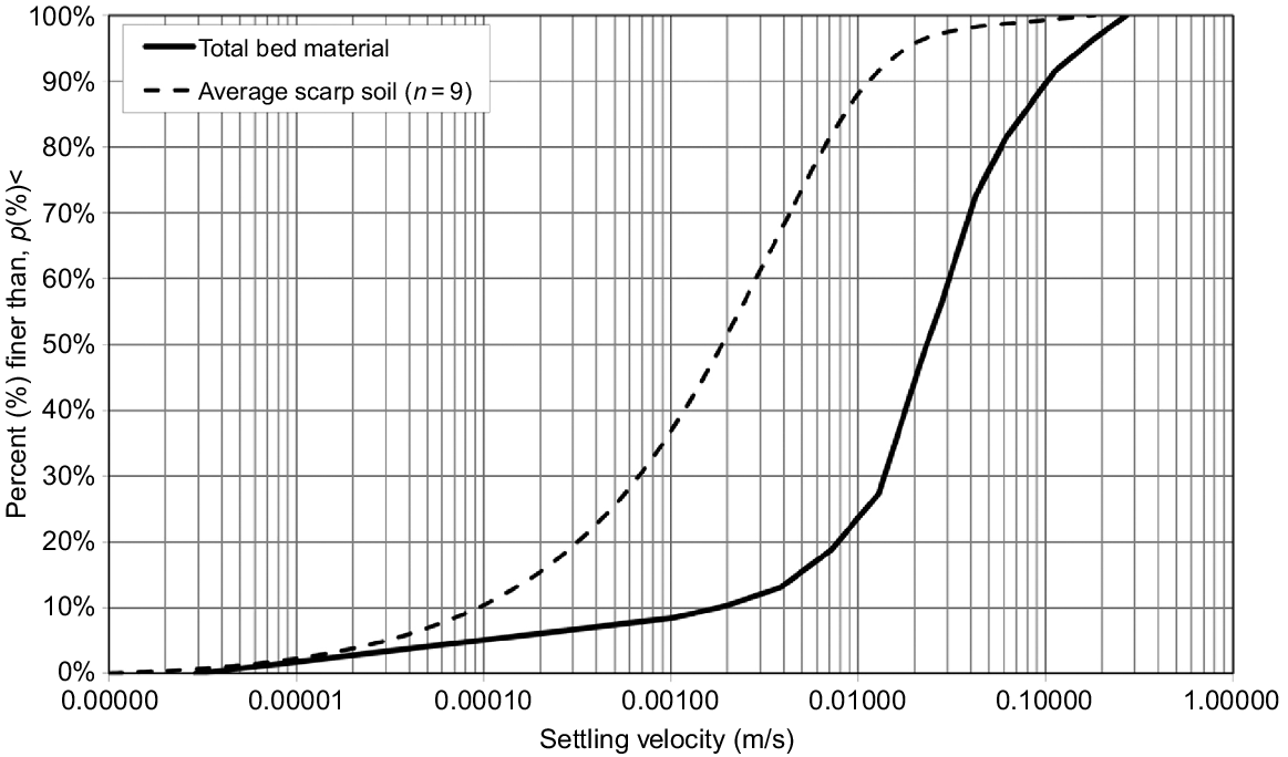
The settling velocity characteristic of sampled material can alternatively be measured using the pipette technique for finer silt and clay size material (Day 1965), or the general modified bottom withdrawal method of Lovell and Rose (1988). The SVC of a surface soil can be affected by how it is wetted and by sediment transportation processes. Such changes in SVCs during rainfall-driven erosion were examined by Hairsine et al. (1999), with structural breakdown due to rainfall impact found to be but one of the reasons for change with time in SVC of the discharged sediment. However, for soil material sampled in situations of flow-driven erosion (such as shown in Fig. 1), SVCs are generally relatively stable through an erosion event.
Denoted by ci, the spatially-averaged sediment concentration of particles (or aggregates) of settling velocity class is defined by fall velocity vi. Then by definition, the rate of deposition di of this class is given as follows:
which can be summed over the entire range of settling velocity classes to give the total rate of deposition, ∑di. If observations allow definition of a vertical profile of ci to be recorded – as in river observations, e.g. Haddadchi and Rose (2022) – then Eqn 1 can be improved by multiplying the right-hand size of the equation by a factor αi ≥ 1, where αici is the sediment concentration adjacent to the soil bed:
Comment on soil erosion model types
Following extensive measurement of soil and water loss from bounded ‘runoff plots’, especially in the USA, a methodology was developed to summarise the data obtained recognising the rainfall, plot characteristics, crop management and erosion control practices in place. This methodology, called the Universal Soil Loss Equation by Wischmeier (1970), while limited in its ability to describe erosion processes, provided a useful way of summarising data collected from runoff plots, and most importantly as a management tool to help farmers make decisions on what conservation to use to minimise erosion (Wischmeier and Smith 1978).
The more recent main stream of soil erosion models are in the form of deterministic differential equations combining the description of hydraulic and soil erosion processes involved, all within a framework of mass conservation of water and of each size class of sediment, as illustrated later in Eqn 3. However, in contrast to this main approach, Lisle et al. (1998) demonstrated that important insights into rainfall-driven erosion are revealed by a conceptually quite different and independently developed stochastic type of model to describe the processes involved. This approach recognised that the time spent by a particle in shallow rainfall-driven overland flow cannot be neglected in comparison to the time spent by the particle resting on the soil surface. This stochastic approach is shown in Rose et al. (1998) to be totally compatible with the previously developed deterministic model of Hairsine and Rose (1991), but also clarifies the associated dynamics of sediment size or settling velocity with sediment transport. That eroded sediment often ends up polluting streams and rivers, and is an issue of increasing concern and threat to water quality, and particle size plays an important role in such impacts. Finer particles commonly carry the majority of adsorbed chemicals such as plant nutrients or pollutants, settle more slowly and so travel further than coarser sediment components.
Another important outcome of the stochastic approach of Lisle et al. (1998) is that it clearly demonstrates the build-up of a deposited layer, which was described earlier, formed by sediment that was previously detached by rainfall impact. This layer grows in depth during the erosion process providing some protection or cover to the original soil bed from ongoing rainfall impact. This development of a ‘deposited layer’ was experimentally demonstrated by Heilig et al. (2001). The presence of this layer is shown in section ‘The models of Hairsine and Rose’ to have significant consequences, both for sediment concentration as well as its size distribution.
A general feature of most soil erosion models is to express both mass conservation of overland flow and suspended sediment concentration in one downslope dimension. To describe the hydraulics, a one-dimensional kinematic representation is commonly applied. This equation is then accompanied by an expression describing the mass conservation of transported suspended sediment concentration of the following form (e.g. Sander et al. 2011):
where h is flow depth (m), c is concentration of suspended sediment (kg m−3), t is time (s), q is volumetric flow per unit width (m2 s−1), x is downslope distance (m), Dr is net rate of soil removal by rainfall impact and Df is net rate of removal by overland flow; these rates being the difference between removal and deposition rates (which can therefore be positive or negative). Expressions for Dr commonly involve rainfall rate, rainfall kinetic energy or momentum.
Many erosion models treat the soil surface being eroded as though it exhibits a common and unchanging resistance with depth to whatever erosion mechanisms are operating on it. This assumption is made in the models EUROSEM (Morgan et al. 1998), LISEM (De Roo et al. 1996), KINEROS2 (Smith et al. 1995) and WEPP (Flanagan and Nearing 1995). In these widely used models, deposition is not represented as a continuous ongoing process operating in its own right. As a consequence of this assumption, Df in Eqn 2 is described using a term called ‘transport capacity’, a factor used by the above-mentioned authors to distinguish between situations of net erosion and net deposition. Such use of the term ‘transport capacity’, which does not make the physically necessary distinction between these two processes, means the term is not unique, and this leads to the difficulties and uncertainties in such model application as described by Polyakov and Nearing (2003). As further explained by Sander et al. (2007) and Sander et al. (2011) it should be a requirement of physically-based erosion modelling to distinguish between, and separately describe, erosion processes and sediment deposition as quite different physical processes, each depending on different physical characteristics.
Despite such uncertainties, the models listed in the above paragraph have been widely used with significant practical success and utility, especially WEPP, which has had the implementation support of the United States Department of Agriculture. Despite the physical limitations of the models listed, their use has been of considerable practical application in erosion assessment and control.
In contrast to the models listed in the preceding paragraphs, the unique erosion process multi-size class modelling approach of Hairsine and Rose (1991, 1992a, 1992b), often referred to as HR models, recognises that sediment deposition requires description as a quite separate process. It is this ongoing process of deposition that forms the dynamic layer of deposited material described earlier, which has distinctly different and much weaker physical characteristics than the original soil matrix. This insight holds true whether the erosion mechanism involved is rainfall impact or overland flow, or a combination of both erosion processes. In either erosion context the soil removed settles back to the soil surface, no longer in its original cohesive state, but in a state which offers no significant cohesive resistance to any further removal. It then follows that the erosive power exerted on the soil surface is partitioned between (a) removal of sediment from the upper cohesionless layer, in which energy is expended only in lifting such sediment up into the overlying water layer, and (b) removal of cohesive soil from the lower originating cohesive soil profile. Since separate rate equations are given for all the mechanisms involved in erosion dynamics, this approach does not require the flawed ‘transport capacity’ concept common to the models referred to earlier. Rather, in the HR approach, the ‘transport capacity’ emerges naturally as the unique outcome of equating separately described erosion and deposition processes.
The models of Hairsine and Rose
Close observation of field erosion processes provided an important basis for these models, conceived as being physically-based descriptions of observed processes. It was nevertheless recognised to be of great importance that model effectiveness be tested under the fully-controlled conditions which can be provided by a tilting flume-simulated rainfall facility, which gives complete control over inflow onto and rainfall application to uniform bodies of chosen soil types. It was the results of such controlled experimentation which enabled evaluation of the two important physically-defined, but unknown parameters in the models.
The observed formation of an upper cohesionless deposited layer is an important common feature of all the following three models: whether erosion is rainfall-driven (Hairsine and Rose 1991), driven by sheet flow (Hairsine and Rose 1992a) or is flow-driven with rills (Hairsine and Rose 1992b). The possibility of mass flow driven by gravity, as in landslides, is acknowledged but not considered in these models.
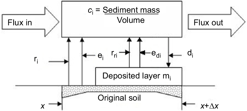
Fig. 2 shows the conceptual flow diagram of the HR models for general sediment size class i, including both rainfall-driven and flow-driven erosion processes. Note that the rate of deposition (di) contributing to the development of the deposited layer is explicitly represented as a quite separate physical process adding to the deposited layer. This recognition is in contrast to the implication of Eqn 3 where it is only net rates that are recognised.
Flow diagram illustrating the sediment fluxes occurring between the overlying sediment flux, the underlying compact soil bed and the covering deposited layer formed by deposition. Terms ei and edi represent the rainfall detachment rates from the original un-eroded soil surface and the deposited layer, respectively. Terms ri and rri are the entrainment and re-entrainment rates from the original and deposited layers, respectively (after Hairsine and Rose 1992a).
When the processes of flow-driven entrainment and re-entrainment are dominant, it is widely recognised that the source of erosive power is the excess of streampower (Ω) (or rate of working of the flow-induced shear stresses) over a threshold value Ω0 (or Ω−Ωo). It is found that only some fraction (F) of this excess streampower is effective in causing erosion, with the remaining fraction (commonly about 90%) lost to passive sources such as heat and noise. It is this available excess streampower that in turn is then fractionally distributed between the re-entrainment of sediment from the upper-lying deposited layer, and entrainment of sediment from the underlying original cohesive soil (a process assumed to occur independently of sediment size class).
The process of re-entrainment is shown as taking place from the covering cohesionless sediment layer (Fig. 2), a layer formed by the sediment size-selective process of deposition (as shown by Eqn 1). Mass conservation is expressed in the theory for each sediment size in the deposited layer as also ensured for each sediment size in the flow above the deposited layer (cf. Fig. 2). Hairsine and Rose (1992a) should be consulted for the conservation equations involved.
A most important outcome of recognising the presence of this deposited layer is that it sets an upper limit, termed the ‘transport limit’, to sediment concentration (ct). This limiting situation occurs when the deposited layer completely envelopes and protects the underlying original cohesive soil from erosion. The sediment concentration at this limit is therefore the highest that can possibly be experienced in the particular flow condition which applies. An expression for ct is quite simply derived by recognising that the energy expended per second in re-entrainment is given by the product of the immersed weight of sediment lifted, and the distance through which it is lifted, a distance taken to be the depth of water (D) above the deposited layer. The power required to support this re-entrainment comes from the effective fraction F of the local streampower Ω = ρgSDV, where S is land slope and V is velocity of flow; expressing this equality symbolically yields an expression for re-entrainment rate. At the transport limit this re-entrainment rate must be equal to the rate of deposition given by Eqn 1, this equality resulting in the following equation for the transport limit:
where vav is the average sediment settling velocity, and σ and ρ are the densities of sediment and water, respectively. In this context it is found to be a reasonable assumption to regard the threshold streampower (Ω0) as negligible compared to streampower (Ω).
If protection from flow-driven erosion of the underlying soil matrix provided by the upper deposited layer is not complete, then the resultant sediment concentration is dependent both on the degree of that protection, and also on the resistance to entrainment offered by the underlying compact soil layer – that is by the strength of the original soil matrix. The resultant sediment concentration achieved in this general situation is commonly referred to as ‘entrainment limiting’, though since its value depends on the degree of partial protection provided by the covering layer, which can vary, this is not a general ‘limiting’ value in the same definite sense as is the ‘transport limit’.
For dynamic erosion under steady sheet-flow, solutions of all the full relevant equations have been given by Hairsine and Rose (1992a), Sander et al. (2007) and Hogarth et al. (2011). A much simpler but approximate solution for the general ‘entrainment limiting’ conditions has been provided by Rose et al. (2007), together with experimental justification of its acceptable accuracy. In all erosion investigations, the physically defined parameters in the theory are commonly unable to be independently measured since no methods are available to do so. Therefore, these physically meaningful and useful parameters must be evaluated by optimisation to provide the best fit between model prediction and the experimental data.
The HR models describe the settling velocity of soil by a probability density function. This choice provides complete freedom to choose the number of size classes that are to be considered – a distinct advantage, since the settling velocity distribution of many soils can vary over several orders of magnitude. Being freely able to represent this possible wide size range is of great importance in modelling the transport of agricultural chemicals for example, since these are commonly bound to a wide range of finer soil fractions.
The theories of Hairsine and Rose in particular have been critically investigated experimentally using the Griffith University Tilting-Flume Simulated Rainfall Facility (GUTSR), described by Misra and Rose (1995). This facility allows a uniform layer of soil that is placed in a 6 m long tilting flume to be subject to combinations of (a) controlled inflow onto the top of the flume and (b) controlled simulated rainfall – either separately or in combination. Having such precise control of the erosion context and its consequences allows accurate and critical investigation of erosion processes, and comparison with their modelling representation.
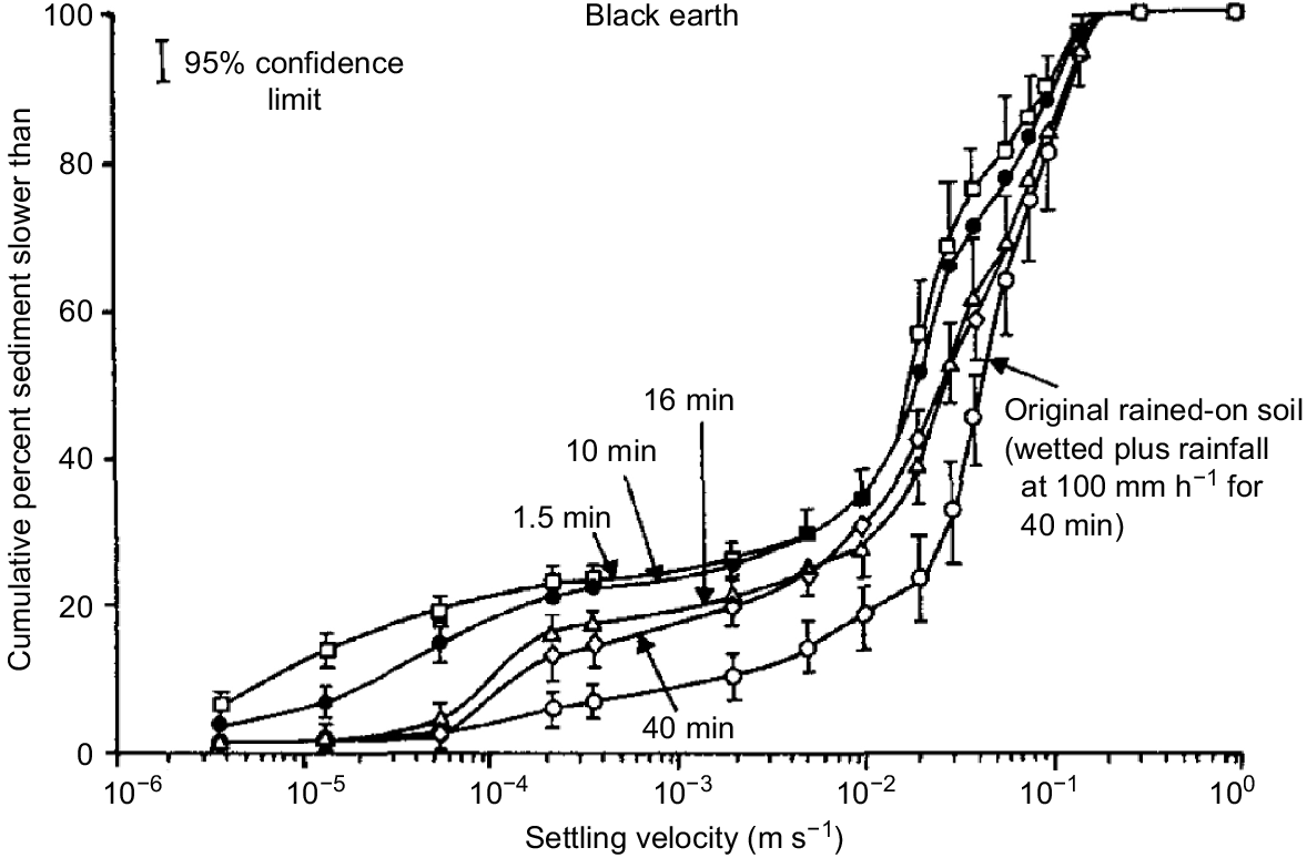
Flume experiments with rainfall-dominated erosion were reported by Proffitt et al. (1991), showing that, even under steady rainfall, sediment concentration declines with time. This decline was accompanied by a progressive coarsening of initially finer eroded sediment, with sediment settling-velocity characteristics finally approaching that of the original soil, a feature illustrated in Fig. 3. This progressive coarsening in sediment through time is due to the finer and slower settling sediment being transported more rapidly than coarser components. Since plant nutrients are commonly associated with the finer fractions, it is this sorting process which is a common source of the nutrient enrichment commonly observed in eroding sediment, an issue investigated for example by Palis et al. (1990a).
Mean settling velocity distribution of a rained-on Vertisol (or black earth), measured after selected periods of exposure to rainfall at a rate of 100 mm h−1. Also shown is the settling velocity of the original soil, which had been exposed to the same rainfall for 40 min (from Proffitt et al. 1993).
The results given by Proffitt et al. (1991) also support the previously mentioned gradual build-up of a layer of coarser deposited material; this layer increases in thickness until it may provide complete protection of the original soil from rainfall impact. This interpretation of the experimental data received modelling support from Sander et al. (1996) and Hairsine et al. (1999).
The GUTSR facility has also been employed in investigating the situation where soil erosion is due to overland flow alone, providing data to test the predictions of the appropriate theory of Hairsine and Rose (1992a, 1992b), as updated by Sander et al. (2007). Such evidence of support was provided by Sander et al. (1996) and Rose et al. (2007) using dynamic soil erosion data obtained during steady sheet-flow over three very different soil types.
Term F, the fraction of the excess streampower effective in erosion, is one of the factors in the overland flow theory that requires experimental evaluation for the particular circumstances to which the theory is being applied. Another factor requiring evaluation in describing flow-driven erosion is J (J kg−1), the specific energy of entrainment of the original soil matrix; J is the amount of energy required to entrain unit mass of the original cohesive soil. Using the GUTSR facility, Proffitt et al. (1993) investigated the consistency of the evaluated factors F and J for a range of contrasting soil type and management conditions using overland flows that covered a range of rilled as well as non-rilled hydraulic conditions. Over the range of turbulent flow conditions and soil types investigated, the value of F was found to be relatively constant, depending on the particular erosion context involved. In this same study, data for the lower (or source limit) condition yielded consistent values for the second parameter requiring determination, J, which reflects the cohesive soil strength of the particular original soil involved in the experiments.
The consistency in the evaluated values of F and J found in these experiments contributes to the confidence in the physical basis of the HR model approach. However, the experimental demands to evaluate such parameters foreshadow the likely need for some simplification in the theory in applying the HR model in most field-scale applications – an issue taken up later in section ‘Methodologies for the study of soil erosion management at field scales’ of this paper.
It is generally assumed that in situations where overland flow is the dominant source of erosion, the development of rills leads to a higher concentration of sediment than would occur if rills did not develop. However, a study of the role of the geometry and frequency of rectangular rills by Fentie et al. (1997) showed that, despite the increased streampower due to rilling, this does not in all cases result in a higher sediment concentration.
So far in this section the emphasis has been on outlining the basis of the Hairsine and Rose set of erosion models, and in testing their utility under controlled and dynamic conditions. Subsequent sections of this review provide some examples of where such theory has provided the basis of important and practically-oriented dynamic field soil conservation investigations, for example of gullies, both of alluvial (section ‘‘Transport Limit’ behaviour in alluvial gullies’) and hillside (section ‘Modelling classical colluvial or hillside gullies’) form. The HR modelling also forms the basis of a new physically-based method of measuring soil strength variation in a soil profile (section ‘Soil strength – its role and measurement’) and in field soil erosion management investigations (section ‘Methodologies for the study of soil erosion management at field scales’).
Van Oost et al. (2004) well illustrate the experimental and analytical difficulties that need to be overcome in applying soil erosion models, of the type discussed in this section, to cultivated field contexts with complex topography and runoff influenced by cultivation channels.
The following section describes an important large-scale naturally-occurring field situation in which sediment concentration has been found to be consistently at the ‘transport limit’ (as defined above) over a very wide range of flow conditions.
‘Transport limit’ behaviour in alluvial gullies
The term ‘transport limit’ continues to be used in the sense defined in section ‘The models of Hairsine and Rose’ as the quasi-steady state sediment concentration resulting from equality between the rates of sediment deposition and re-entrainment. The ‘transport limit’ is thus achieved when the supply of erodible sediment is unrestricted by source strength considerations, as distinct from the more common situation where erosion rate is described as ‘supply-limited’.
This section outlines an important and extensive fluvial context where transport limiting behaviour has been found to be persistent, leading to extensive damaging landscape erosion features and also to serious pollution of rivers and streams to which the eroded sediment is conveyed. This concentrated type of erosion feature is commonly called an ‘alluvial gully’ to distinguish it from the more narrowly incised ‘colluvial’ (or hillside) type of gully.
While alluvial gullies can be found world-wide, particular research attention has been given to these extensive gully systems in the tropical Australian regions of Queensland and Western Australia (Brooks et al. 2009). Sediment from such gully systems is then delivered downstream by rivers, so being a major source of coastal and barrier reef pollution and damage (Haynes et al. 2007). In these regions, cattle grazing is a major land use and alluvial gullies are commonly initiated by cattle tracking down steep riverbanks for water. The resultant confined erosion feature (or gully head) develops following the line of the cattle pad, extending upslope to initiate a much more expansive erosion feature, or scarp, in which erosion spreads rapidly because the soil in this previously undisturbed low-slope floodplain is commonly a sodic red and yellow earth, of fine-grained silt/clay texture. This extensive floodplain area is highly erodible, and serious erosion is induced even by the modest grazing pressure imposed by the large-scale cattle grazing practised. Once erosion commences, the extensive floodplain scarp becomes a major source of fine sediment, to which at the gully exit is added a coarser particle component (i.e. coarse silt and sand) sourced from the exit channel or gully head.
In this context, Shellberg et al. (2013) described a detailed study of the sediment production, characteristics and yield over a range of time scales from an alluvial gully that delivered sediment from a more extensive upslope 33 ha scarp-bounded area carved out of the flood plain. The gully site is one of thousands located in the Mitchell River megafan in northern Queensland, Australia. Hydrological measurements and sediment sampling were carried out at a gauge site on the incised outlet of the alluvial gully, which had an approximately rectangular cross section of rather constant width. Water discharge (Q) was calculated from measurements of water velocity, channel width and flow depth made at both rising and falling stages. Sediment samples were collected over a range of discharges and then separated into silt/clay and sand fractions, with the results collated into rating curves of both suspended sediment concentration and water depth (Fig. 4). The noticeable lack of any hysteresis in these relationships is consistent with sediment transport being at the transport limit.
Rating curves at a gauge station in an alluvial gully in a Mitchell River megafan, northern Queensland, Australia. Shows relationships between water depth (D) and discharge (Q) for water years 2009 and 2010, Q and suspended silt/clay concentration, Q and suspended sand concentration, and Q and total suspended sediment concentration (SSC) for both years combined (Rose et al. 2015).
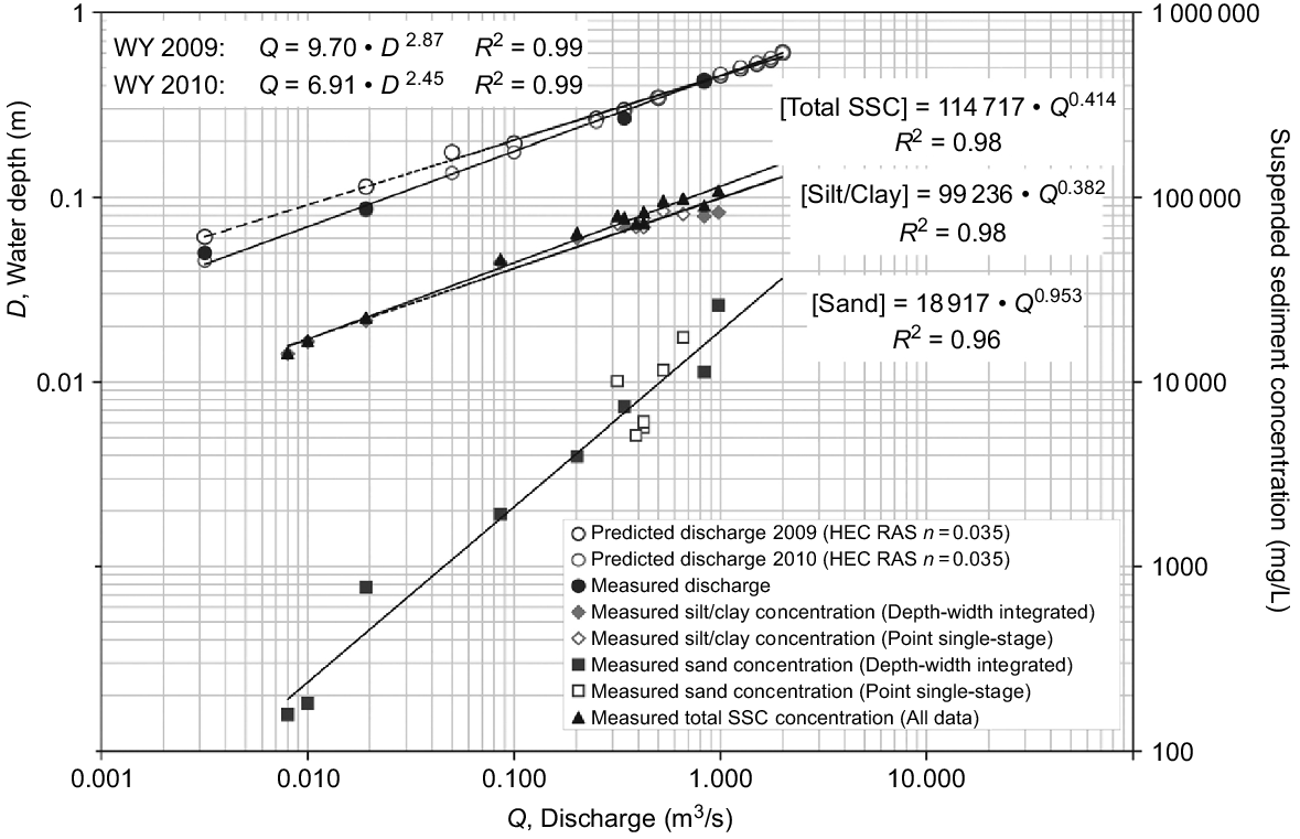
The expanding low slope and scarp-bounded area is the major source of the eroded finer soil fractions, with rainfall detachment and washload transport playing roles in this complex and devastating erosion complex. The coarser sand fraction had origins closer to the measurement site (Shellberg et al. 2013). These authors describe how the settling velocity characteristics of the two sediment components shown in Fig. 4 were combined to evaluate the increase with discharge Q in the average settling velocity, vav, of the entire sediment, a term required to calculate the transport limiting sediment concentration ct (Eqn 4). As shown in Fig. 4, the sediment concentration of the coarser sand fraction increases more rapidly with Q than the fine silt/clay fraction, and it follows that vav will increase with Q.
The only other term in Eqn 4 required to calculate ct is F, the streampower efficiency factor. Adopting a value of F ≈ 0.032 gave no discernible difference between sediment load calculated using the transport limiting theory of Hairsine and Rose (1992a) and the values of sediment load, either measured by occasional direct field sampling or continuously inferred from observational load history.
Using the transport limiting theory of Hairsine and Rose (1992a) (given in Eqn 4) to interpret these data, it was found that, over the entire seasonal runoff record, the sediment concentration measured at the gully exit gauge site was indeed consistently at the transport limit ct.
This finding encourages possible success in the future of predicting sediment loss from the vast range of alluvial gullies located in similar dispersible soil floodplains, based on the measurement (or rainfall-based estimates) of their accumulated runoff. Rehabilitation of such eroded land is a demanding land management priority, but such activity operates in a context of deciding whether such land use is sustainable in this type of geophysical and soil type context.
Modelling classical colluvial or hillside gullies
The origins and characteristics of the commonly observed colluvial or hillside gully provide many contrasts as well as some similarities to the alluvial gullies described in section ‘Transport limit’ behaviour in alluvial gullies’.
The development of colluvial or hillside gullies commonly results from the interaction of landscape characteristics and land management changes. Those landscape features that act to collect and concentrate runoff, when combined with either reduction in vegetative cover or soil disturbance, tend to increase the likelihood of colluvial gully initiation. The development of any such gully then depends on the local hydrological history and the resistance which the soil profile offers to the erosion processes – that is, the strength of the soil profile.
While gully erosion can be found in most if not all countries, their widespread occurrence in Australia has been clearly related to land management practices introduced by European settlement (Prosser et al. 2001). Saxton et al. (2012) analysed aerial photographic and LIDAR records of gullies in sub-tropical south-east Queensland, together with rainfall and flow records, to seek a better understanding of the potential mechanisms of gully formation. Daily rainfall records extending back to 1900 were also used to follow trends through time. One important finding was that rates of extension of gullies (m2 year−1) were found to increase close to linearly with the product of gully catchment area and land slope. Gully catchment area is expected to be correlated with average water flow, and slope to be a factor increasing sediment concentration during gully erosion. Thus, the finding of a linear relationship with the product of these two factors suggests that the potential for gully development can be understood in process terms over the geographical range of gullies observed.
It is the difficulties in collecting information through time, particularly on the hydraulics of flow as well as the resultant geometrical development of the gully, that limits the development, application and testing of gully erosion models.
The classical gully reported here was located in one of 12 sub-catchments (or cells) whose runoff contributed to the formation of the headwaters of the Bremer River in south-east Queensland. The accumulating flow of this river was continuously monitored at a location that captured the combined output from the 12 cells contributing runoff to the river. Rainfall rate, assumed typical for all flow-contributing cells, was continuously monitored at a central site. Rose et al. (2014) should be consulted for the details of how it was possible to construct a realistic estimate of the hydrograph for flow down the gully for each of the 11 runoff events over the 2-year recording period between successive LIDAR captures of gully geometry, which were recorded to an accuracy of some 0.15 m in vertical resolution.
Each hydrograph was expressed in terms of an effective equivalent steady-state discharge rate for each rainfall event. This flow rate was then used to compute the average sediment concentration at the transport limit during each runoff event, quantities used in later analysis.
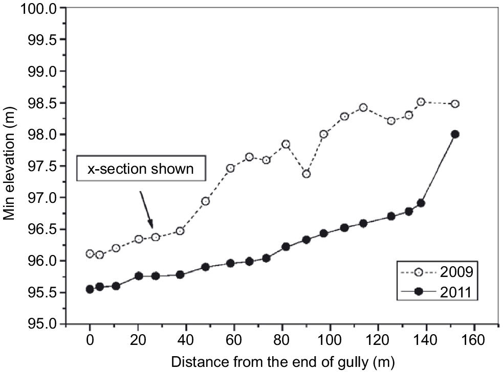
Repeated LIDAR observations defined both the longitudinal and cross-sectional profiles of the gully, the longitudinal profiles being given in Fig. 5. Using all such gully profile information, Fig. 6 shows the longitudinal variation in volumetric erosion intensity over the 2-year measurement period.
Longitudinal profile of the lowest elevation along the gully in 2009 and 2011 that feeds sediment into the Bremer River, south-east Queensland, Australia (from Rose et al. 2014).
Longitudinal variation in erosion intensity over the 2-year measurement period for the Bremer River gully, south-east Queensland, Australia (from Rose et al. 2014).
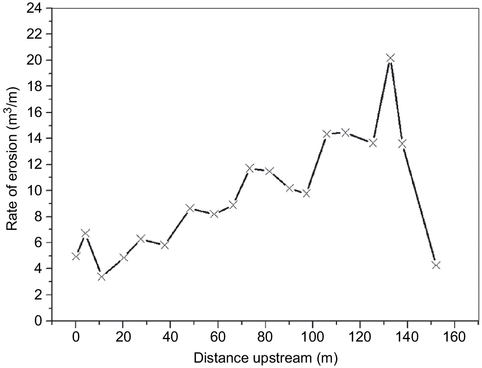
Observation confirmed that the rapid increase in erosion intensity over the first 20 m of the gully head was most likely due to the complete collection of water input to the gully over that length, and that it was the resultant combination of streampower and the waterfall effect that caused the observed intensive erosion over that section of the gully head.
The theory developed in Rose et al. (2014) to interpret all these data on both the hydrologic input and resultant erosion of the gully was an adaption of that given by Hairsine and Rose (1992a, 1992b). Equal erosion contributions from streampower and the upslope waterfall effect over the gully head section were assumed. The ‘waterfall effect’ was modelled in terms of the kinetic energy achieved by incoming water to the gully falling from the surrounding soil surface down through the depth of the gully. No explicit recognition was given to the possible role of gravity-driven processes or gully-wall collapse as an additional source of sediment input to the gully.
Downstream of the gully head, flow-driven erosion was assumed to be the only erosion process, modelled using the simplifying assumption that by the time sediment reached the end of the gully the deposited layer had reached a state of equilibrium between re-entrainment and deposition. This approximate assumption was later replaced by a more accurate development of the model by Roberts (2020). Given the approach outlined earlier, the only unknown in application of the theory was the overall resistance to erosion offered by the soil (J), defined as the energy required in Joules to remove 1 kg of soil. A value of J = 406 J kg−1 gave good agreement between predicted and estimated soil loss based on successive LIDAR observations of the increase in the gully volume. This value of J would clearly be an effective average value since there would be some variation in soil strength with depth down the profile. The simplifying assumption referred to may also affect this estimated average value of J.
Since data on gully width and length change over time are far more available from aerial photography than from LiDAR data, Rose et al. (2014) also examined the possibility of using this less-detailed source of gully geometry information to provide a less certain, but still useful estimate of J. The question of how the value of J can be directly measured as a function of depth in the soil profile is addressed in the section ‘Soil strength – its role and measurement’ of this review.
The model of Roberts (2020) has also been applied to consider the likely advantage of possible conservation options designed to reduce erosion in an eroding hillside gully. This role of modelling application holds the promise of most useful practical outcomes. Roberts et al. (2022) also provided a comprehensive, though selective, review of the mathematical modelling of classical (or permanent) gullies, illustrating key features of gully types. The governing equations are also summarised for those models seeking to provide physically-based descriptions of gully erosion processes. This review concluded that much more progress is needed in this area of endeavour, both in model development and in gaining the data to test model ability to predict gully behaviour. Illustrating some methods of gaining the data required for model testing has been a major objective of this section of the review.
Soil strength – its role and measurement
There is a very wide range of research and established methodologies in estimating the strength properties of soil. Interest in soil strength ranges very widely – examples arising in concerns for loadbearing, tillage resistance and root penetration, as well as soil erosion. The particular focus of this section of the review is the in-situ soil strength profile involved when soil is subject to the erosive processes of flowing water.
Section ‘Modelling classical colluvial or hillside gullies’ describes a methodology for evaluating the overall or average value of J for the complete soil profile exposed during the development of a hillside or classical gully. However, considerable profile variation in J is the norm.
In the context of assessing the in situ erodibility profile of soil, a standard experimental approach is known as the ‘jet erosion test’ or JET test, which involves use of a submerged jet as described by Hanson and Cook (2004). To interpret such data, the commonly-used analysis method is in terms of the product of excess shear stress and an erodibility coefficient. Despite the extensive use of this method of analysis of test data, the relevant literature reports evidence of a lack of consistency in the results obtained with this approach. As a result of this inconsistency, Marot et al. (2011) introduced a new theoretical approach to such data interpretation by considering the fate of the energy provided by the submerged jet. This general type of approach was developed in a quite different manner by Rose et al. (2018), and then applied in field studies by Haddadchi et al. (2018).
This section describes this relatively new method for determining the spatial variation in J with depth into any soil profile using data obtained with the standard mini-JET tester equipment. Fig. 7 is an example, taken from Haddadchi et al. (2018), of the average scour profiles for a specially-prepared soil profile of uniform strength characteristics. Excavated volume was measured at five successive times during the JET experiment. Haddadchi et al. (2018) can be consulted for the experimental technique used in obtaining such spatial profile data.
Average scour volumes and their standard error for the uniform soil experiment at the five times of scour geometry measurement (from Haddadchi et al. 2018).
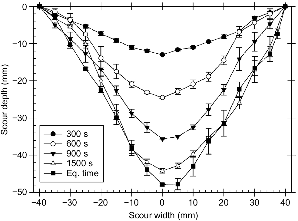
While the mass of soil removed in jet scour can be determined directly by collection, the alternative of measuring excavation volume and determining bulk density is commonly used. It is not uncommon for jet excavation profiles to be somewhat symmetrical in shape as illustrated in Fig. 7. If so, a convenient method of calculating excavation volume for any jet penetration depth(s) is to assume a generalised Gaussian shape, a method described in Rose et al. (2018).
At the commencement of a JET test, all the kinetic energy of the jet is initially expended in eroding the exposed soil surface. However, as erosion proceeds to carve a cavity into the soil, an increasing fraction of the jet energy becomes dissipated in a variety of energy-dissipating mechanisms; this fraction of energy dissipation becoming 100% at maximum jet penetration into the soil body.
Following Hairsine and Rose (1992a), the rate of decline of energy involved in eroding cohesive soil depends on the product of the resistance to erosion offered by the soil, J (J s−1), and the mass rate of soil detachment (dm/dt), a rate that was evaluated in JET tester experiments by the product of bulk density and rate of increase in measured excavation volume (dV/dt). For field soil profiles, the value of J will commonly increase with the penetration, s (m), of the jet into the soil, and is therefore denoted J(s).
As introduced above, the analysis makes the basic assumption that, regardless of the soil type being investigated, the rate of energy expenditure in eroding soil, R(s), is based on rate of removal of soil mass as given by Eqn 5:
where ρb is appropriate bulk density, m is mass and V is soil volume excavated by the jet. While the value of component terms in Eqn 5 will be quite varied for different soil profiles, the product of these disparate terms defines R(s).
In the unique approach described by Rose et al. (2018), the value of J as a function of depth in the field soil of interest, i.e. J(s), is obtained by comparing the rate of energy decline in any field soil profile with the energy decline in a specially-prepared laboratory soil bed constructed in such a manner that soil strength is strictly constant with depth in that soil bed. This constancy in J is recognised by its value being denoted Jconst. The rate of decline in jet energy involved in penetrating and eroding soil in this uniform profile is then described, in a manner following the general Eqn 5, as follows:
In Eqn 6, the term (a + f(s)) is a fitted polynomial relationship that describes the measured rate of decline in penetration volume V (i.e. dV/dt) with scour depth (s) and ρbc is the bulk density of this uniform referring soil profile. The geometrical form of this polynomial for the uniform soil profile is shown as the upper curve in Fig. 8. Note that a is the value of dV/dt for s = 0. How the constant value, Jconst, can be determined is described later.
Illustrative example of experimentally-derived functions of dV/dt vs scour depths for both an upper Brisbane River field soil (denoted UBR) and for the uniform soil sample (from Rose et al. 2018).
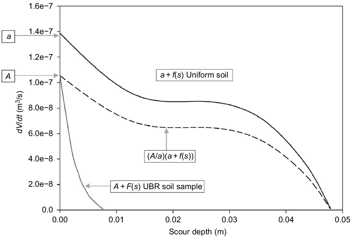
The rate of decline in jet penetration volume measured using JET equipment at any field site of interest can be similarly determined, with results described by the polynomial form (A + F(s)), as shown in Fig. 8. In a similar manner to Eqn 6, the rate of jet energy expenditure in eroding the field soil can then be written as follows:
where Js is the depth-variable value of J, (A + F(s)) is the appropriate polynomial describing the rate of volume penetration for the field profile investigation (an example is given in the lowest curve in Fig. 8) and ρb is soil bulk density.
Since Eqn 5 applies regardless of soil type we can equate the two expressions for R(s) given in Eqns 6 and 7, and then solve this equality for the unknown (but sought after) profile of values for Js, as follows:
As discussed in Rose et al. (2018), it is desirable to multiply the right-hand side of Eqn 8 by a minor correction factor if (as is commonly the case) the jet kinetic energy differs slightly between the field profile investigation and that used in the uniform soil experiment yielding the value of Jconst. Both polynomial expressions in Eqn 8 are experimentally determined (as illustrated in Fig. 8), and Jconst is then calculated as described below.
As the constant known jet energy (Rjet) impinges on the initial surface of the prepared uniform soil, all the jet energy will be expended in eroding soil at a rate which, as follows from Eqn 6, is given by Jconstρbca. Thus, the profile-constant value of Jconst is given as follows:
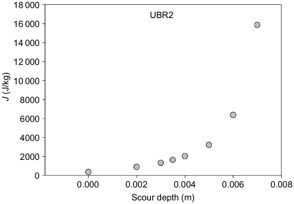
With Jconst thus determined, then Js for the field soil profile can be calculated for the experimentally-explored value of s using Eqn 8. An example of the increase in Js with scour depth s is given in Fig. 9 for the same field site whose results for dV/dt are given as the lower curve in Fig. 8. As expected in field soil profiles, the value of Js rises quite rapidly with penetration depth s.
Plot of J(s) versus scour depth s for soil profile UBR2 on the upper Brisbane River, obtained using Eqn 8 (from Haddadchi et al. 2018).
The summary given here of the two papers listed earlier in this section demonstrates the vital contribution of obtaining data for a specially-prepared soil test sample of strictly uniform soil strength properties; it is against the behaviour of this particular test soil that the soil-strength characteristics of any (however non-uniform) field soil can be evaluated.
It is of particular importance to recognise that the application of the analysis methodology described here is quite independent of the particular characteristics of the uniform test soil employed. It therefore follows that the data presented in table II of Haddadchi et al. (2018) on the properties of the uniform reference soil described in that publication can also be employed in exactly the same way by any user of the methodology of soil strength evaluation described in the two publications on which this summary is based. That is, the methodology outlined here (and in the two papers referred to) is of quite general application and is available to any user of JET soil investigation equipment.
Haddadchi et al. (2018) also discuss field experience in using JET equipment at a range of riverine profile sites.
Methodologies for the study of soil erosion management at field scales
The physically-based soil erosion models of Hairsine and Rose outlined in section ‘The models of Hairsine and Rose’ involved soil erodibility parameter J (J kg−1), the energy required to erode unit mass from the soil matrix which generally underlies a weak deposited layer. Publications reviewed in that section indicated that in order to evaluate the value of J appropriate to any erosion event, the resulting sediment concentration (c, kg m−3) must be followed as a function of time during the erosion event. Unfortunately, due to technological limitations in field studies, this time-variable measurement is usually unavailable. This poses the question: how can a good estimate of the value of J be determined in field erosion studies in which only information on an average value () of sediment concentration is available?
A solution to that question is illustrated by an international study of erosion in the tropical steep lands of Southeast Asia and Australia (Coughlan and Rose 1997). This multi-country collaborative program was partially supported by the Australian Centre for International Research (ACIAR), and was designed to assess the effectiveness of locally-chosen cropping systems designed to reduce soil loss to a deemed acceptable level.
Technology overview
The technology developed and successfully employed in this ACIAR project is summarised by Ciesiolka et al. (1995) and Coughlan and Rose (1997). For plots up to a size of some 200 m2, the technology employed for the measurement of flow rate was of the ‘tipping bucket’ type; for larger plots, measurement of flow rate was achieved using the calibrated depth of flow on a flume located at the plot outlet. With either type of flow rate measurement, data recording used on-site data logging equipment. Total soil loss from the experimental bounded plots was determined as the measured sum of two components. The highly depositable or ‘bedload’ component was collected in a shallow collecting trough at the bottom of each plot. This trough also served to direct or divert the outflowing finer sediment-bearing runoff through either a tipping bucket or flume for continuous flow rate recording. A continuous small-sediment sample was bled from this outflow, yielding an estimate of the flow-weighted average sediment concentration of that outflow. This sediment concentration was converted to an event soil loss, to which was added the physically collected ‘bedload’ soil loss to provide data on the total event soil loss for the relevant plot and runoff event. Rainfall rate and soil depositability (or vav) for the eroded sediment were separately measured.
Overview of erodibility estimate
As discussed in section ‘The models of Hairsine and Rose’, and defined in Eqn 4, an upper or ‘transport limit’ (ct) to sediment concentration occurs when the original cohesive soil matrix is completely covered by a cohesionless soil layer formed by deposition of eroded soil. With measurements as described in the ACIAR experiments, ct can be calculated for any measured flow velocity V (ms−1). However, when some of the effective streampower is utilised in eroding soil from the resistant soil matrix then sediment concentration will be less than ct, how much less depends on the ‘erodibility’ (J) of the soil matrix. When technology limitations such as described above prevent direct estimate of J, a most useful empirical surrogate for J, termed beta (β) was found to provide a way of describing soil erodibility, which had the conceptual advantage of having an intimate relation with J, a relationship illustrated in Fig. 10. The erodibility parameter β, introduced by Rose (1993), is defined by the following relationship:
where ct is the sediment concentration at the transport limit.
Sediment concentration (c) calculated as a function of streampower (Ω) for particular illustrative values of parameter J and β. The relationships for the selected values of J are calculated from the theory of Hairsine and Rose (1992a), assuming that sediment concentration remains at the source limit corresponding to the chosen values of J (from Rose 1993).
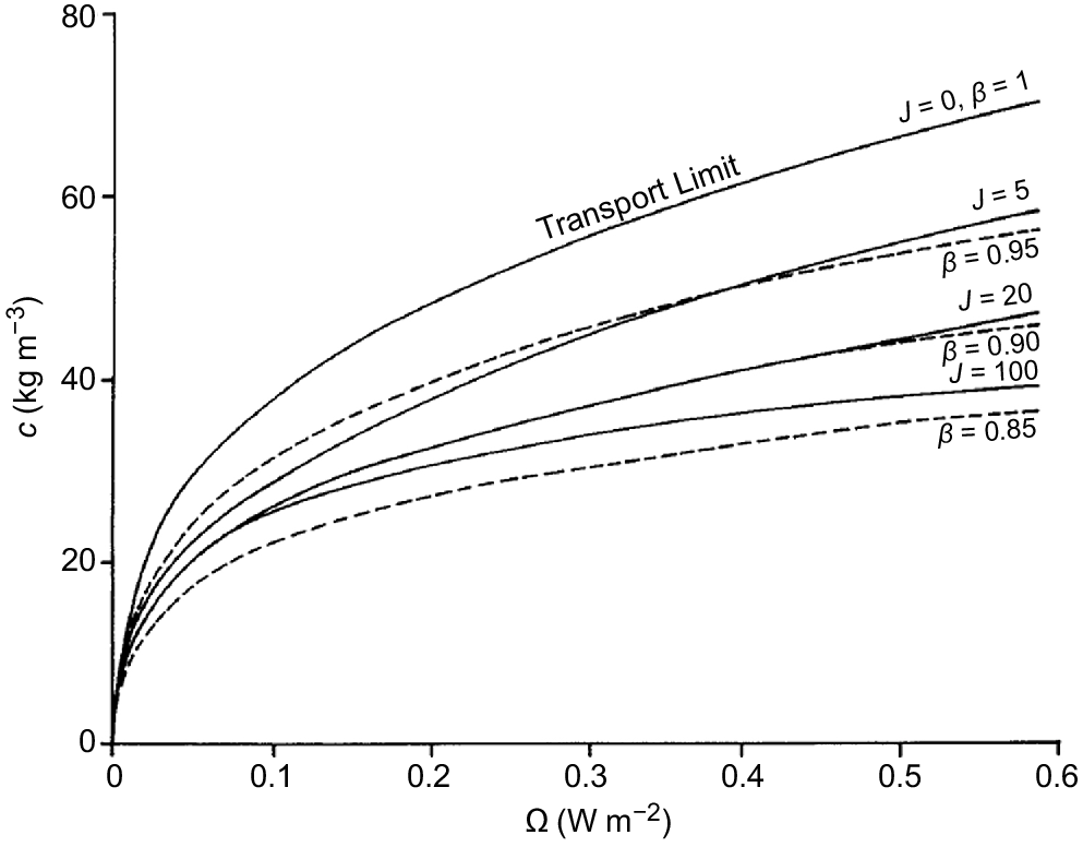
Fig. 10 shows that as soil strength J increases from zero at the transport limit, β decreases from 1 and in a manner displaying formal similarity to J in its trend with Ω. This similarity in form in the relationship between c and β and c and J adds confidence in using this empirical erodibility parameter β.
With the field data limitations described earlier, it is only the average value of c (i.e. ) that is available. Thus Eqn 10 needs adaption to apply, not only to time-variant quantities, but also to event-average sediment concentration values, so that:
where is the event average sediment concentration obtained from event totals of both sediment loss and overland flow. With measured, and calculated as shown in Ciesiolka et al. (1995), then an event-average value of β can be calculated:
It follows that the soil loss (SL) up to any stage of an erosion event is given as follows:
where the summation extends up to the stage of interest.
If the soil in the plot being investigated is bare, then the lower that the value of β is below unity, the lower the erodibility of the soil (see Fig. 10). If the plot under investigation is subject to some soil conserving practice, then the lower the value indicated for β, the more effective is the soil conserving option being evaluated.
Results obtained in the multi-country study showed that β generally declined with a finer texture of the soil being eroded. Even for soil in a particular plot, erodibility varied with time. The full results obtained with application of these methodologies in collaborating Southeast Asian countries, including Australia, are described in a special issue of Soil Technology (1995) and in Rose et al. (2010).
Routing sediment from erosion sources to sinks
Models of erosion processes on linear landscape elements, such as those reviewed in sections ‘Comment on soil erosion model types’ and ‘The models of Hairsine and Rose’ of this review, do not seek to represent all aspects of source-to-sink geomorphic processes. To address these limitations, dynamic models connecting erosion sources, sediment transport and transient storage are required. These models should adequately represent geomorphic processes, such as deposition and re-entrainment of sediment within the channel or in floodplains, sediment connectivity in river network and transport of eroded materials with different size ranges.
Sediment routing systems link the fate of eroded materials from sources to reservoirs and sinks through the river network (Allen 2017). Sediment routing models can be useful for catchment sediment management by providing mass of sediment deposited in the riverbed, and in tracking sediments through their transport pathways within the river network. When coupled with catchment hydrological models, with estimates of continuous flow records for whole river network, sediment routing models can capture the dynamics of sediment transport in space throughout the catchment river network, as illustrated by the following examples.
Various sediment routing models have been developed to determine sediment generation, mostly at a reach scale, which refers to a segment of river between points of confluence/bifurcation and its contributing area. Beveridge et al. (2020) developed a network sediment routing model that connects processes of stochastic hillslope sediment supply with bedload and suspended load sediment transport and deposition across a channel network.
Czuba (2018) introduced a Lagrangian framework on a previously developed network-based bed material sediment transport model that connects sediment sources and sinks (Czuba and Foufoula-Georgiou 2014; Czuba et al. 2017). This framework allows transport of mixed-size sediment in a river network using daily flow data to determine continuous sediment transport. The model was adapted by Ahammad et al. (2021) to simulate mixed-size sediment pulse behaviour with downstream river geomorphic variations.
Schmitt et al. (2016) developed a sediment connectivity model, CASCADE, which considers transport of eroded materials from individual catchment sources using separate transport and deposition processes for each source. The ability of modelling multiple grain-sizes was added by Tangi et al. (2019), and a dynamic version of this routing model that can investigate the spatiotemporal evolution of sediment supply and transport was developed by Tangi et al. (2022).
Gilbert and Wilcox (2020) developed an approach for modelling the reach-scale sediment dynamics at the catchment scale using easily accessible geospatial data with a capability of simulating flood-plain exchange dynamics. The model uses flow data to determine temporal variations in sediment across the river network.
Sediment routing systems that aim to connect erosion sources to sinks need to be based on the principle of mass conservation. Despite the simplicity of this concept, its application may be challenging, especially in complex catchments with various geomorphic processes, as observed in quantifying sediment budgets (Hinderer 2012; Grams et al. 2013).
There are important erosional situations, such as in the geomorphic consequences of extreme flooding of compound river channels, where modelling must recognise the essential two-dimensional nature of the hydraulics involved. Sharpe and Kemp (2021) used two-dimensional hydraulic software (BMT 2018) to determine the hydraulic thresholds involved in the serious disruption of tree and grass vegetation in the compound channels of a sub-tropical river in Australia. These thresholds were identified by comparing the results of alternative possible hydraulic thresholds with the geomorphic and vegetational damage observed using repeat LIDAR surveys before and after extreme flooding. Observations of an increase in severity and frequency of flooding has been associated with the consequences of global warming.
Erosion control practices and soil conservation
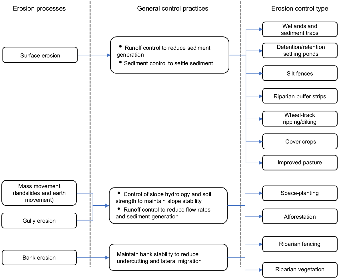
After evaluating the erosion processes within any catchment and determining the impact of such sediment loss on downstream aquatic environments, the next step in catchment management is to identify potential erosion control practices. As outlined in Fig. 11, different erosion control practices can be used for different types of erosion processes.
Minimum tillage
Conservation agriculture is a broad concept and policy area covering a wide range of desirable principles and objectives, one of which has particular relevance to soil conservation and erosion control: this is to minimise tillage to that necessary for establishment of the desired product or crop. This concept of minimum tillage covers a spectrum of activities, with a lower bound of what is described as direct drilling or zero-till. Minimum tillage is the use of primary and/or secondary tillage necessary for meeting crop production requirements under the existing soil and climatic conditions. Adoption of some form of such practices in grain-growing areas of Australia is described in an extensive review by Llewellyn and D’Emden (2010). Their review showed that while adoption of no-till by a participating farmer was usually not complete, it commonly exceeded 70%, and that the overall proportion of growers using some amount of no-till commonly exceeded 90%. While Australia seems to be somewhat outstanding in its degree of adoption of some form of minimum tillage, such practices have also been helpful in reducing soil loss in countries as varied as South Africa (Taylor et al. 2012) and Austria (Komissarov and Klik 2020), all without loss in productivity compared with conventional tillage (defined as primary and secondary tillage operations in preparing a seedbed and/or cultivating a crop grown in a given area).
Soil contact cover
Soil conservation is concerned with ways in which the surface of the planet can be managed to meet food needs sustainably by minimising the loss soil and its nutrients. There are two different broad types of land use where the importance of maintaining an adequate degree of cover of the soil surface is well recognised.
Pastoral land
With pastoral land use, the main management task is to limit grazing pressure so as maintain an adequate degree of soil protection by the pasture. Controlled animal rotation can be one effective method of achieving this aim, a management method more likely to be adopted in more productive contexts because of fencing costs, and the shepherding requirements involved. Sanjari et al. (2009) present the results of a time-controlled grazing and soil erosion catchment-scale experiment in which sediment was shown to be significantly reduced by 65–90% as the pasture cover increased due to controlled grazing over the 6-year experimental period. The corresponding observed decrease in runoff was proportionately less than the observed decrease in sediment loss.
Cultivated land
A second common type of land use involves cultivation of some kind. The aim of soil conserving practices is to both minimise soil disturbance to that which is necessary, and at the same time maintain as much cover of the soil surface as is possible. In agricultural contexts, cover which can minimise erosion of the soil surface can come from two distinct sources: aerial cover provided by vegetation against rainfall impact, and surface contact cover consisting, for example, of mulch from vegetative material in contact with the soil surface. Surface contact cover provides protection against both rainfall impact and erosive effects of overland flow and also encourages infiltration.
Especially in the more-humid tropics, a common challenge is caused by increasing population pressure causing large tracts of hilly land to be brought into use for intense agricultural use. A typical example is the Philippines, where high rainfall intensities, steep slopes and commonly uncertain land tenure can lead to very high erosion rates and land degradation (Paningbatan et al. 1995; Presbitero et al. 1995). Both these publications arose from the ACIAR-supported investigations introduced previously in section ‘Methodologies for the study of soil erosion management at field scales’ of this review. Paningbatan et al. (1995) describes the soil-conserving alley-cropping management system investigated at Los Banos in the Philippines in which metre-wide hedgerows of leguminous shrub perennials were planted along the contour, and whose trimmings provided surface contact cover for the annual crops planted between the hedgerows. The shrub hedgerows also provide a porous barrier, reducing sediment loss and encouraging infiltration. Compared to common up-and-down slope and weed-free farmer cultivation, annual soil loss was reduced by this soil conserving management system from 150 to less than 5 t ha−1 year−1.
Fig. 12 summarises results on the effect of various degrees of surface contact cover provided by crop residues and hedgerow trimmings in experiments at Los Banos on the ratio of sediment concentration (c) with any level of contact cover to the concentration from a bare plot (cb). In this figure, contact cover was provided by crop residue trimmings from contour-planted hedgerows. The scatter shown in the relationship reflects the difficulty in estimating the degree and effectiveness of surface contact cover.
The sediment concentration ratio c/cb as affected by various forms of surface contact ratio – reproduced from fig. 4 of Paningbatan et al. (1995) with permission by Elsevier.
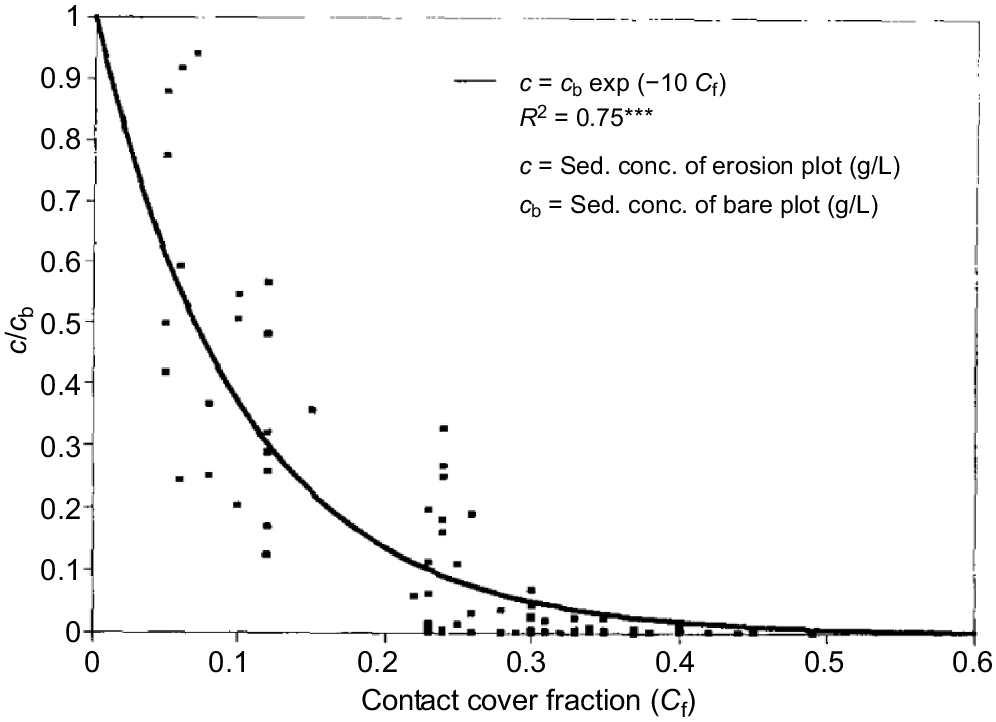
The relationship shown in Fig. 12 is well related by the following general fractional form:
where k = 10 and Cf is the surface contact cover fraction.
Loss of plant nutrients in soil erosion, such as organic nitrogen, was shown by Palis et al. (1990a) to depend on the level and type of surface contact cover, as well as the dominant erosion source (i.e. either rainfall detachment or entrainment by runoff).
Contour banks (or check dams)
In addition to providing surface contact cover in its various forms, a common method of land management designed to limit soil loss from cultivated fields is to intercept runoff and its sediment load from a field in an almost horizontal contour bank or check dam as schematically illustrated in Fig. 12. Possibly the most extensive use of such structures is in China, where Xu et al. (2020) report the presence of over 100 000 such structures in the Loess Plateau alone. These authors also report on the various theories and practices implemented extensively in many areas of China, where high population levels provide the need for intensive agriculture on productive areas of soil. Xu et al. (2020) also describe the difficulty in monitoring the time-varying processes involved, and the limitations experienced in adopting modelling approaches designed to guide contour bank construction. A result of such difficulties has been the common use for such purposes of empirically-based practices derived from the extensive field experience and observations in China.
Fig. 13 illustrates, in geometrically simplified form, common features of contour bank design in which sediment loss from the field area captured by the contour channel is not designed to be complete, since complete capture would ensure a limited life for the contour bank. Thus, as illustrated in Fig. 13, it is common for the channel to be constructed with a low slope so as to allow some fraction of the captured sediment to be dispersed to a safer location for deposition.
Illustrating the flow of water and sediment from a plane land element to a channel (Qc) as in a graded channel – reproduced from fig. 11 of Rose (1985).
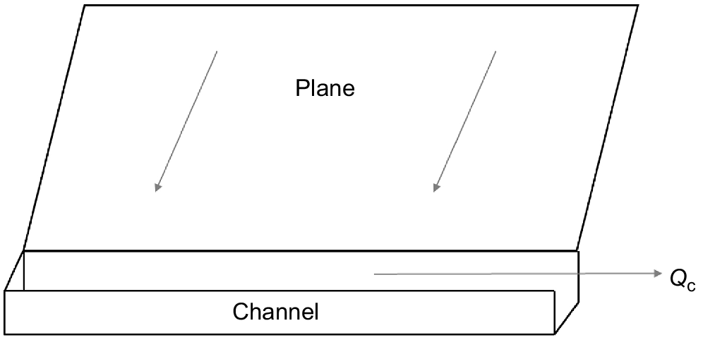
Using the contour bank design shown in Fig. 13, Rose (1985) applied soil erosion/deposition theory as discussed in section ‘The models of Hairsine and Rose’ to describe the hydrologic and sediment transport processes involved in this system. One useful outcome of this theory is an equation [numbered (57) in Rose (1985)] for the sediment loss ratio, ϕ, which is defined as follows:
where the sediment settling velocity, vi (m s−1), is distributed over I equal size classes, and Qc (m s−1) is the runoff rate per unit area of the channel.
The accuracy of Eqn 15 has been tested using data from Loch and Donnollan (1983) obtained on a field whose clay loam soil was classified as a Udic Pellustert. Using data on the distribution of vi and the history of Qc measured for a channel slope of 0.3%, the value of ϕ (expressed as a percentage) was 14%, very close to the value obtained by direct measurement of the sediment fluxes involved.
While it is of course preferable that the installation of contour banks or check dams should not be the only aid used in reducing soil loss, it does provide such support, it is a practice widely adopted internationally and not only in the context of mechanised agriculture.
Terracing
Terracing is a term describing a somewhat more nuanced soil conservation practice compared to the contour bank system described in section ‘Contour banks (or check dams)’, though in general both systems are designed to reduce the runoff from sloping land accumulating and causing serious erosion. While ‘terracing’ can involve many different forms of soil conserving practices, it commonly involves a much more frequently placed channelling of excess rainfall across slope to safe disposal compared to that in contour bank systems. In assessing the suitability of soil conserving practices in China, Liu et al. (2013) illustrate the necessity of considering socio-economic as well as technical factors in their design.
Kirkby and Morgan (1980) outline the many various types of terraces, including the commonly used contour or diversion type of terrace. These are commonly called parallel terraces in the USA, so named because they are constructed parallel to each other and with a gentle downward slope. They are commonly cultivated as a part of the field, with minimum interference to other farming operations. Indeed, tillage equipment may be the main or only source of equipment used in such terrace formation. Due to terrace construction with a gentle downward slope, excess water which accumulates behind the terrace is commonly discharged safely off the cultivated area, perhaps to an adjacent downslope grassed waterway.
Conclusion
Modelling soil erosion involving water has progressed from the Universal Soil Loss Equation data summary approach to a range of modelling activity that seeks to mathematically describe the physical erosion processes involved. The section ‘Comment on soil erosion model types’ in this review summarises the significant number of such approaches, making the case that the approach described by Hairsine and Rose provides a more accurate representation of the physical processes involved in water-driven soil erosion. This is partly because this model is unique in recognising sediment deposition as a distinct ongoing process that forms an upper cohesionless soil layer above the coherent soil layer from which it has been derived by whatever erosion processes are involved. This modelling approach has been substantially validated for both rainfall and run-off driven erosion by substantial stimulated rainfall/flume studies, and extensively applied in ACIAR-supported field erosion studies across several Southeast Asian countries and in Queensland (Coughlan and Rose 1997). These field studies allowed quantitative evaluation of the soil loss reduction produced by a wide range of soil conserving options.
These extensive field studies involved the measurement of total event soil loss and the rates of runoff and rainfall. However, it is recognised that the technology required for these rate measurements is not commonly available. Thus, one ongoing challenge is to use the data obtained in these detailed ACIAR studies to assess the accuracy of less technology-demanding methods of estimating runoff and soil loss. Useful progress in this objective of developing and accessing less data-demanding methods of runoff and soil loss prediction has been given by Yu et al. (1997).
A soil conserving option adopted in the Philippines is the introduction of a leguminous hedgerow between the major arable crop. This resulted in a reduction in soil loss greater than would be expected by the observed reduction in runoff, evidently due to sediment retention (Paningbatan et al. 1995). The effectiveness of such buffer strips is worthy of more detailed investigation (Hussein et al. 2007).
There is great concern, especially in Australia, at the serious damage being done to coral in the Great Barrier Reef due to sediment transported downstream to it by rivers. The origin of much of this sediment is from alluvial gullies, commonly initiated by cattle tracking to rivers for water (Doriean et al. 2021). Gully remediation, while shown to be possible, is very expensive. Therefore, urgent efforts are currently being made to rank the significance of the vast number of alluvial gully sediment sources so as to prioritise the limited available treatment. This very demanding task would be greatly assisted if the finding that sediment transport in such gullies can be at the transport limit, as shown by Rose (2017), proves to be a common feature of alluvial gullies. If so, then this great task can be considerably simplified to that of ranking their hydrologic delivery – still a daunting task.
Forestalling the development of any type of gully, whether alluvial or hillside in nature, is most desirable but involves complex social and management issues. However, the model of hillside gully erosion developed by Roberts (2020) is being successfully applied to effectively and inexpensively evaluate the potential benefit or limitations of alternative possible gully remediation measures which might be adopted. This continues to illustrate the power and utility of erosion modelling.
Interpreting the strength of in-situ soil profiles using the commonly employed JET test equipment has been beset with the distortion of using non-physically-based methods of data interpretation. The model of Rose et al. (2018) has overcome this limitation, and the data given in the companion paper by Haddadchi et al. (2018) referred to in section ‘Soil strength – its role and measurement’ provide the basis for quite general application of this much-improved method of data interpretation.
The predictions of climate change modelling include greater amounts and higher rates of rainfall. This gives a warning that the design of soil conserving systems currently used in agriculture require re-assessment of their adequacy to provide protection in a future with more erosive conditions. Erosion modelling must play a role in seeking to meet such challenges. Even commonly practised conservation measures, such as terracing, require design re-evaluation of their ability to provide adequate protection under such harsher erosive conditions.
References
Ahammad M, Czuba JA, Pfeiffer AM, Murphy BP, Belmont P (2021) Simulated dynamics of mixed versus uniform grain size sediment pulses in a Gravel-Bedded River. Journal of Geophysical Research: Earth Surface 126(10), e2021JF006194.
| Crossref | Google Scholar |
Beveridge C, Istanbulluoglu E, Bandaragoda C, Pfeiffer AM (2020) A channel network model for sediment dynamics over watershed management time scales. Journal of Advances in Modeling Earth Systems 12(6), e2019MS001852.
| Crossref | Google Scholar |
Brooks AP, Shellberg JG, Knight J, Spencer J (2009) Alluvial gully erosion: an example from the Mitchell fluvial megafan, Queensland, Australia. Earth Surface Processes and Landforms 34(14), 1951-1969.
| Crossref | Google Scholar |
Cheng N-S (1997) Simplified settling velocity formula for sediment particle. Journal of Hydraulic Engineering 123(2), 149-152.
| Crossref | Google Scholar |
Ciesiolka CA, Coughlan KJ, Rose CW, Escalante MC, Hashim GM, Paningbatan EP, Jr, Sombatpanit S (1995) Methodology for a multi-country study of soil erosion management. Soil Technology 8(3), 179-192.
| Crossref | Google Scholar |
Cuthbertson A, Dong P, King S, Davies P (2008) Hindered settling velocity of cohesive/non-cohesive sediment mixtures. Coastal Engineering 55(12), 1197-1208.
| Crossref | Google Scholar |
Czuba JA (2018) A Lagrangian framework for exploring complexities of mixed-size sediment transport in gravel-bedded river networks. Geomorphology 321, 146-152.
| Crossref | Google Scholar |
Czuba JA, Foufoula-Georgiou E (2014) A network-based framework for identifying potential synchronizations and amplifications of sediment delivery in river basins. Water Resources Research 50(5), 3826-3851.
| Crossref | Google Scholar |
Czuba JA, Foufoula-Georgiou E, Gran KB, Belmont P, Wilcock PR (2017) Interplay between spatially explicit sediment sourcing, hierarchical river-network structure, and in-channel bed material sediment transport and storage dynamics. Journal of Geophysical Research: Earth Surface 122(5), 1090-1120.
| Crossref | Google Scholar |
De Roo APJ, Wesseling CG, Ritsema CJ (1996) LISEM: a single-event physically based hydrological and soil erosion model for drainage basins. I: theory, input and output. Hydrological Processes 10(8), 1107-1117.
| Crossref | Google Scholar |
Doriean NJC, Bennett WW, Spencer JR, Garzon-Garcia A, Burton JM, Teasdale PR, Welsh DT, Brooks AP (2021) Intensive landscape-scale remediation improves water quality of an alluvial gully located in a Great Barrier Reef catchment. Hydrology and Earth System Sciences 25(2), 867-883.
| Crossref | Google Scholar |
Fentie B, Rose CW, Coughlan KJ, Ciesiolka CAA (1997) The role of the geometry and frequency of rectangular rills in the relationship between sediment concentration and stream power. Soil Research 35(6), 1359-1378.
| Crossref | Google Scholar |
Gilbert JT, Wilcox AC (2020) Sediment routing and floodplain exchange (SeRFE): a spatially explicit model of sediment balance and connectivity through river networks. Journal of Advances in Modeling Earth Systems 12(9), e2020MS002048.
| Crossref | Google Scholar |
Grams PE, Topping DJ, Schmidt JC, Hazel JE, Jr., Kaplinski M (2013) Linking morphodynamic response with sediment mass balance on the Colorado River in Marble Canyon: issues of scale, geomorphic setting, and sampling design. Journal of Geophysical Research: Earth Surface 118(2), 361-381.
| Crossref | Google Scholar |
Haddadchi A, Rose CW (2022) A physically based model of deposition, re-entrainment, and transport of fine sediment in gravel-bed rivers. Water Resources Research 58(8), e2021WR031782.
| Crossref | Google Scholar |
Haddadchi A, Rose CW, Olley JM, Brooks AP, McMahon J, Pietsch T (2018) An alternative method for interpreting JET erosion test (JET) data: Part 2. Application. Earth Surface Processes and Landforms 43(3), 743-754.
| Crossref | Google Scholar |
Hairsine PB, Rose CW (1991) Rainfall detachment and deposition: sediment transport in the absence of flow-driven processes. Soil Science Society of America Journal 55(2), 320-324.
| Crossref | Google Scholar |
Hairsine PB, Rose CW (1992a) Modeling water erosion due to overland flow using physical principles: 1. Sheet flow. Water Resources Research 28(1), 237-243.
| Crossref | Google Scholar |
Hairsine PB, Rose CW (1992b) Modeling water erosion due to overland flow using physical principles: 2. Rill flow. Water Resources Research 28(1), 245-250.
| Crossref | Google Scholar |
Hairsine PB, Sander GC, Rose CW, Parlange J-Y, Hogarth WL, Lisle I, Rouhipour H (1999) Unsteady soil erosion due to rainfall impact: a model of sediment sorting on the hillslope. Journal of Hydrology 220(3-4), 115-128.
| Crossref | Google Scholar |
Hanson GJ, Cook KR (2004) Apparatus, test procedures, and analytical methods to measure soil erodibility in situ. Applied Engineering in Agriculture 20(4), 455-462.
| Crossref | Google Scholar |
Hashim GM, Ciesiolka CAA, Yusoff WA, Nafis AW, Mispan MR, Rose CW, Coughlan KJ (1995) Soil erosion processes in sloping land in the east coast of Peninsular Malaysia. Soil Technology 8(3), 215-233.
| Crossref | Google Scholar |
Haynes D, Brodie J, Waterhouse J, Bainbridge Z, Bass D, Hart B (2007) Assessment of the water quality and ecosystem health of the Great Barrier Reef (Australia): conceptual models. Environmental Management 40(6), 993-1003.
| Crossref | Google Scholar | PubMed |
Heilig A, DeBruyn D, Walter MT, Rose CW, Parlange J-Y, Steenhuis TS, Sander GC, Hairsine PB, Hogarth WL, Walker LP (2001) Testing a mechanistic soil erosion model with a simple experiment. Journal of Hydrology 244(1-2), 9-16.
| Crossref | Google Scholar |
Hinderer M (2012) From gullies to mountain belts: a review of sediment budgets at various scales. Sedimentary Geology 280, 21-59.
| Crossref | Google Scholar |
Hogarth WL, Rose CW, Parlange JY (2011) Erosion caused by overland flow: an interpolation method. Journal of Hydrology 402(1–2), 155-158.
| Crossref | Google Scholar |
Hussein J, Yu B, Ghadiri H, Rose C (2007) Prediction of surface flow hydrology and sediment retention upslope of a vetiver buffer strip. Journal of Hydrology 338(3–4), 261-272.
| Crossref | Google Scholar |
Komissarov MA, Klik A (2020) The impact of no-till, conservation, and conventional tillage systems on erosion and soil properties in lower Austria. Eurasian Soil Science 53(4), 503-511.
| Crossref | Google Scholar |
Lisle IG, Rose CW, Hogarth WL, Hairsine PB, Sander GC, Parlange J-Y (1998) Stochastic sediment transport in soil erosion. Journal of Hydrology 204(1–4), 217-230.
| Crossref | Google Scholar |
Liu G, Dai F, Nan L, Du S (2013) Assessing the suitability of soil and water conservation practices in Southwestern China. Land Use Policy 30(1), 319-327.
| Crossref | Google Scholar |
Loch RJ, Donnollan TE (1983) Field rainfall simulator studies on two clay soils of the Darling Downs, Queensland. II. Aggregate Breakdpwn, sediment properties and soil erodibility. Soil Research 21(1), 47-58.
| Crossref | Google Scholar |
Lovell CJ, Rose CW (1988) Measurement of soil aggregate settling velocities. 1. A modified bottom withdrawal tube method. Soil Research 26(1), 55-71.
| Crossref | Google Scholar |
Marot D, Regazzoni P-L, Wahl T (2011) Energy-based method for providing soil surface erodibility rankings. Journal of Geotechnical and Geoenvironmental Engineering 137(12), 1290-1293.
| Crossref | Google Scholar |
Misra RK, Rose CW (1995) An examination of the relationship between erodibility parameters and soil strength. Soil Research 33(4), 715-732.
| Crossref | Google Scholar |
Morgan RPC, Quinton JN, Smith RE, Govers G, Poesen JWA, Auerswald K, Chisci G, Torri D, Styczen ME (1998) The European Soil Erosion Model (EUROSEM): a dynamic approach for predicting sediment transport from fields and small catchments. Earth Surface Processes and Landforms 23(6), 527-544.
| Crossref | Google Scholar |
Pal D, Ghoshal K (2013) Hindered settling with an apparent particle diameter concept. Advances in Water Resources 60, 178-187.
| Crossref | Google Scholar |
Palis RG, Okwach G, Rose CW, Saffigna PG (1990a) Soil erosion processes and nutrient loss. 1. The interpretation of enrichment ratio and nitrogen loss in runoff sediment. Soil Research 28(4), 623-639.
| Crossref | Google Scholar |
Palis RG, Okwach G, Rose CW, Saffigna PG (1990b) Soil erosion processes and nutrient loss. II. The effect of surface contact cover and erosion processes on enrichment ratio and nitrogen loss in eroded sediment. Soil Research 28(4), 641-658.
| Crossref | Google Scholar |
Paningbatan EP, Ciesiolka CA, Coughlan KJ, Rose CW (1995) Alley cropping for managing soil erosion of hilly lands in the Philippines. Soil Technology 8(3), 193-204.
| Crossref | Google Scholar |
Pimentel D, Harvey C, Resosudarmo P, Sinclair K, Kurz D, McNair M, Crist S, Shpritz L, Fitton L, Saffouri R, Blair R (1995) Environmental and economic costs of soil erosion and conservation benefits. Science 267(5201), 1117-1123.
| Crossref | Google Scholar | PubMed |
Polyakov VO, Nearing MA (2003) Sediment transport in rill flow under deposition and detachment conditions. Catena 51(1), 33-43.
| Crossref | Google Scholar |
Presbitero AL, Escalante MC, Rose CW, Coughlan KJ, Ciesiolka CA (1995) Erodibility evaluation and the effect of land management practices on soil erosion from steep slopes in Leyte, the Philippines. Soil Technology 8(3), 205-213.
| Crossref | Google Scholar |
Proffitt APB, Rose CW, Hairsine PB (1991) Rainfall detachment and deposition: experiments with low slopes and significant water depths. Soil Science Society of America Journal 55(2), 325-332.
| Crossref | Google Scholar |
Proffitt APB, Hairsine PB, Rose CW (1993) Modeling soil erosion by overland flow: application over a range of hydraulic conditions. Transactions of the ASAE 36(6), 1743-1753.
| Crossref | Google Scholar |
Prosser IP, Rutherfurd ID, Olley JM, Young WJ, Wallbrink PJ, Moran CJ (2001) Large-scale patterns of erosion and sediment transport in river networks, with examples from Australia. Marine and Freshwater Research 52(1), 81-99.
| Crossref | Google Scholar |
Roberts ME (2020) MERGE: modelling erosion resistance for gully erosion – a process-based model of erosion from an idealised linear gully. Soil Research 58(6), 576-591.
| Crossref | Google Scholar |
Roberts ME, Burrows RM, Thwaites RN, Hamilton DP (2022) Modelling classical gullies – a review. Geomorphology 407, 108216.
| Crossref | Google Scholar |
Rose CW, Yu B, Ghadiri H, Asadi H, Parlange JY, Hogarth WL, Hussein J (2007) Dynamic erosion of soil in steady sheet flow. Journal of Hydrology 333(2-4), 449-458.
| Crossref | Google Scholar |
Rose CW, Yu B, Misra RK, Coughlan KJ, Fentie B (2010) Use of GUEST technology to parameterize a physically-based model for assessing soil erodibility and evaluating conservation practices in tropical steeplands. In ‘Handbook of erosion modelling’. Eds RPC Morgan, MA Nearing) pp. 195–222. (Wiley Blackwell)
Rose CW, Yu B, Ward DP, Saxton NE, Olley JM, Tews EK (2014) The erosive growth of hillside gullies. Earth Surface Processes and Landforms 39(15), 1989-2001.
| Crossref | Google Scholar |
Rose CW, Shellberg JG, Brooks AP (2015) Modelling suspended sediment concentration and load in a transport-limited alluvial gully in northern Queensland, Australia. Earth Surface Processes and Landforms 40(10), 1291-1303.
| Crossref | Google Scholar |
Rose CW, Olley JM, Haddadchi A, Brooks AP, McMahon J (2018) An alternative method for interpreting jet erosion test (JET) data: part 1. Theory. Earth Surface Processes and Landforms 43(3), 735-742.
| Crossref | Google Scholar |
Sander GC, Hairsine PB, Rose CW, Cassidy D, Parlange J-Y, Hogarth WL, Lisle IG (1996) Unsteady soil erosion model, analytical solutions and comparison with experimental results. Journal of Hydrology 178(1–4), 351-367.
| Crossref | Google Scholar |
Sander GC, Parlange J-Y, Barry DA, Parlange MB, Hogarth WL (2007) Limitation of the transport capacity approach in sediment transport modeling. Water Resources Research 43(2), W02403.
| Crossref | Google Scholar |
Sander GC, Zheng T, Heng P, Zhong Y, Barry DA (2011) Sustainable soil and water resources: modelling soil erosion and its impact on the environment. In ‘MODSIM2011, 19th international congress on modelling and simulation’. (Eds F Chan, D Marinova, RS Anderssen) pp. 45–56. (Modelling and Simulation Society of Australia and New Zealand Inc.)
Sanjari G, Yu B, Ghadiri H, Ciesiolka CAA, Rose CW (2009) Effects of time-controlled grazing on runoff and sediment loss. Soil Research 47(8), 796-808.
| Crossref | Google Scholar |
Saxton NE, Olley JM, Smith S, Ward DP, Rose CW (2012) Gully erosion in sub-tropical south-east Queensland, Australia. Geomorphology 173–174, 80-87.
| Crossref | Google Scholar |
Schmitt RJP, Bizzi S, Castelletti A (2016) Tracking multiple sediment cascades at the river network scale identifies controls and emerging patterns of sediment connectivity. Water Resources Research 52(5), 3941-3965.
| Crossref | Google Scholar |
Sharpe R, Kemp J (2021) Vegetation disturbances and flood energy during an extreme flood on a sub-tropical river. Earth Surface Processes and Landforms 46(14), 2841-2855.
| Crossref | Google Scholar |
Shellberg JG, Brooks AP, Rose CW (2013) Sediment production and yield from an alluvial gully in northern Queensland, Australia. Earth Surface Processes and Landforms 38(15), 1765-1778.
| Crossref | Google Scholar |
Soil Technology (1995) Special issue: soil erosion and conservation. Soil Technology 8(3), 177-258.
| Google Scholar |
Tangi M, Schmitt R, Bizzi S, Castelletti A (2019) The CASCADE toolbox for analyzing river sediment connectivity and management. Environmental Modelling & Software 119, 400-406.
| Crossref | Google Scholar |
Tangi M, Bizzi S, Fryirs K, Castelletti A (2022) A dynamic, network scale sediment (dis)connectivity model to reconstruct historical sediment transfer and river reach sediment budgets. Water Resources Research 58(2), e2021WR030784.
| Crossref | Google Scholar |
Taylor TS, Titshall LW, Hughes JC, Thibaud GR (2012) Effect of tillage systems and nitrogen application rates on selected physical and biological properties of a clay loam soil in KwaZulu-Natal, South Africa. South African Journal of Plant and Soil 29(1), 47-52.
| Crossref | Google Scholar |
Van Oost K, Beuselinck L, Hairsine PB, Govers G (2004) Spatial evaluation of a multi-class sediment transport and deposition model. Earth Surface Processes and Landforms 29(8), 1027-1044.
| Crossref | Google Scholar |
Yu B, Rose CW, Coughlan KJ, Fentie B (1997) Chapter 8: Runoff and soil loss prediction. In ‘A new soil conservation methodology and applications to cropping systems in tropical steeplands’. (Eds KJ Coughlan, CW Rose) pp. 101–110. (Australian Centre for International Technical Report 40: Canberra, Australia)