

A three-dimensional reactive transport model for sediments, incorporating microniches
Łukasz Sochaczewski A , Anthony Stockdale A , William Davison A B , Wlodek Tych A and Hao Zhang AA Department of Environmental Science, Lancaster Environment Centre (LEC), Lancaster University, Lancaster, LA1 4YQ, UK.
B Corresponding author. Email: w.davison@lancaster.ac.uk
Environmental Chemistry 5(3) 218-225 https://doi.org/10.1071/EN08006
Submitted: 17 January 2008 Accepted: 22 April 2008 Published: 19 June 2008
Environmental context. Modelling of discrete sites of diagenesis in sediments (microniches) has typically been performed in 1-D and has involved a limited set of components. Here we present a new 3-D model for microniches within a traditional vertical sequence of redox reactions, and show example modelled niches of a range of sizes, close to the sediment–water interface. Microniche processes may have implications for understanding trace metal diagenesis, via formation of sulfides. The model provides a quantitative framework for examining microniche data and concepts.
Abstract. Most reactive transport models have represented sediments as one-dimensional (1-D) systems and have solely considered the development of vertical concentration gradients. However, application of recently developed microscale and 2-D measurement techniques have demonstrated more complicated solute structures in some sediments, including discrete localised sites of depleted oxygen, and elevated trace metals and sulfide, referred to as microniches. A model of transport and reaction in sediments that can simulate the dynamic development of concentration gradients occurring in 3-D was developed. Its graphical user interface allows easy input of user-specified reactions and provides flexible schemes that prioritise their execution. The 3-D capability was demonstrated by quantitative modelling of hypothetical solute behaviour at organic matter microniches covering a range of sizes. Significant effects of microniches on the profiles of oxygen and nitrate are demonstrated. Sulfide is shown to be readily generated in microniches within 1 cm of the sediment surface, provided the diameter of the reactive organic material is greater than 1 mm. These modelling results illustrate the geochemical complexities that arise when processes occur in 3-D and demonstrate the need for such a model. Future use of high-resolution measurement techniques should include the collection of data for relevant major components, such as reactive iron and manganese oxides, to allow full, multicomponent modelling of microniche processes.
Additional keywords: diffusion, early diagenesis, high resolution, organic matter, redox reactions, sulfide, trace metals.
Introduction
Understanding of the cycling of carbon, nitrogen, manganese, iron and sulfur in sediments is largely based on measurement of solution and solid phase components in vertically arranged slices of cores. The dynamic interactions of the various components have been successfully modelled by coupling the reactions to one-dimensional (1-D) diffusion, with the implicit assumption of horizontal uniformity.[1–3] Although transport and reaction in relation to idealised burrows and mounds has been treated quantitatively (Aller[4] and references therein), processes of bioturbation and bioirrigation are commonly modelled by considering their average effects on transport.[5]
The true heterogeneous nature of the solid phase of sediments, especially at the submillimetre scale, is well recognised, but these variations are implicitly assumed to be averaged within the typical volume (20–100 mL) of a sediment slice.[6] Various techniques have emerged that can measure concentrations of solutes directly, on a small scale, without the volumetric averaging inherent in core slices. They are showing that solute concentrations may vary markedly on a small (submillimetre) scale. Data from planar optodes has demonstrated the temporary development of small spheres (1–2-mm diameter) of anoxia within sediment[7] and at the sediment surface,[8] as particles of highly reactive organic matter consume all available oxygen. Sharp dips in oxygen concentration in otherwise smooth vertical profiles obtained using microelectrodes may be similarly explained.[6]
Two-dimensional maps of concentrations of metals and sulfide, obtained using diffusive gradients in thin-films (DGT),[9–13] have demonstrated that the maxima and minima can occur at discrete sites. These observations are consistent with the idea of microniches, where discrete patches of reactive material bring about pronounced local changes in sediment chemistry.
We define the term microniche as a small-scale location within the 3-D sediment matrix where the geochemical behaviour differs significantly from the average for that depth. An example might be a particle of organic matter or other component (e.g. iron oxide) that has biogeochemical reaction rates that are higher (or lower) than the surrounding environment.[6]
Modelling of microniches
Jørgensen[14] modelled the depletion of oxygen within such niches and concluded that sulfate reduction may occur within pellets as small as 100 μm in diameter. Brandes and Devol[15] modelled numerically the 2-D distribution of oxygen and nitrate by considering their reactions at points of reactive organic material distributed stochastically in a planar grid of 100-μm resolution. The averaged vertical profiles were able to explain the similar penetration of O2 and NO3– observed in porewaters obtained by whole core squeezing at 1-mm resolution. This stochastic approach was extended to 3-D by Harper et al.[16] They showed that the production of dissolved metal ions within local sources (>100-μm diameter) set in sediment acting as a uniform sink for metals resulted in much more sharply defined solute maxima (typically 0.5 mm wide) than would be possible with diffusion restricted to 1-D. Reactive transport models for sediments, which include advective contaminant exchange, have been developed.[17–20] Such models have included 3-D simulations of the effects of various sediment–water interface geometries,[21,22] and these models have been further developed to include the effects of bioirrigation.[23] A 3-D model by Meile et al.[24] was devised to include organic matter diagenesis reactions and was applied to assessing the effect of burrow irrigation on solute distributions. Using this model, the significance of burrowing organisms in locally enhancing penetration of both oxygen and nitrate was demonstrated.
Microniche sources and life-span
As the term microniche can apply to any discrete site of reactive organic matter (OM), it can encompass material from a range of different sources. Microniches can be attributed to decaying organisms (observed using a pH optode[25]), algal aggregates (added to sediment to study sulfidic microniches[12]) and faecal pellets (photographed after resin embedding and thin sectioning of an intact core[26]). Root systems can also generate microniches.[27] Such niches will have a range of different properties. For example: algal aggregates will tend to have a high porosity and a low concentration of authigenic oxides; faecal pellets may possess a peritrophic membrane, be more compact than the ambient sediment (lower porosity), and in some cases have been shown to contain a greater proportion of fine mineral grains than the ambient sediment,[26] potentially affecting tortuosity.
The life-span of niches will depend on OM degradation reaction rates and the supply of oxidants, with niche size affecting oxidant supply to the centre of the niche. The duration of anoxia within a microniche occupying the oxic zone may be unlikely to exceed 2.5 days, as Alldredge and Cohen[28] found little or no O2 depletion in faecal pellets of this age or older. Zhu et al.[25] measured pH at a decaying organism and observed that the generation of protons from the niche was not measurable after ~80 h. These studies indicate that microniches tend to have life-spans of days rather than weeks or months.
Aims and approach
Here we present a dynamic diagenetic model set within a 3-D framework, for the investigation of geochemical processes at microniches. The model’s novelty lies in considering in three dimensions both diffusion and organic matter diagenesis (and associated secondary reactions) in small-scale volumes of sediment. It provides for the generation of vertical concentration gradients according to recent 1-D models, while allowing the definition of localised spherical zones of various diameters that may differ in the concentrations, transport or reactivity of components (microniches).
Engineering software packages such as COMSOL are now being used to model diagenetic processes (e.g. Cardenas and Wilson[21]). Although we could have alternatively built and presented specific model simulations using such a package, we chose to develop a self-contained, flexible model, capable of representing a wide range of microniche environments, which will be made freely available. It incorporates a graphical user interface (figure included as Accessory publication), which allows geochemists with no prior modelling expertise to set up and run quite complex problems within a few hours. It can be used to model observed field data or to test hypotheses. In contrast to traditional 1-D models, e.g. Berg et al.,[3] the model is not intended to be used to investigate sediment at the ‘bulk’ scale, where transport by biota needs to be considered. Therefore, features such as tubes, and the transport processes associated with them (e.g. irrigation or advection) are not incorporated. In practice, the small, mm-scale features being modelled may occur between burrows. Consequently, on the timescales of a few days that characterise the lifetime of microniches, they and the burrows can be regarded as separate entities. Consistent with this view, bioturbation may be responsible for relocating a microniche, while not affecting the physical properties of its localised domain. As sedimentation will not be significant over the timescale of days, it is not considered. Validation was achieved by comparison of model outputs with known analytical solutions. Examples of distributions of solutes in the vicinity of microniches of a range of sizes (1–5 mm) are shown. We show the effect of microniches on solute concentrations within and around niches that are positioned close to the sediment–water interface within ambient oxic and suboxic sediment.
Model formulation
Modelling in 3-D presents conceptual and computational challenges. The models must be geochemically sound with respect to transport and reactions, while allowing specific examples of heterogeneity (microniches). The model we have developed uses existing understanding of reaction and transport gained from measurements and modelling in 1-D. A similar system that allows input and simulation of vertical profiles of components was constructed within a 3-D framework. Spherical zones that represent microniches may be created at any location within the 3-D grid (based on the principle that microniches in nature are likely to be introduced at various depths by the actions of biota). As the lifetime of microniches is generally relatively short (days), we focussed on short spatial scales (sub-mm to cm) and times, and disregarded longer-term processes such as sediment recruitment and accumulation. The ultimate aim was to model the heterogeneous distribution of a range of components in sediments in response to the existence of microniches. To achieve this goal, it was necessary to consider the oxidation of OM and all associated redox processes normally considered in diagenetic models. To allow ease of use, an executable form of the model was developed with a graphical user interface (GUI). Flexibility was preserved by allowing the user to define all reactions and the initial spatial setup. The result is a versatile model for considering solute transport and reaction dynamics in sediments (known as 3-D TREAD), which can be used for a wide range of applications.
The model was divided into three modules: a GUI to allow user-friendly control of the simulation setup, a Calculation Unit where all simulations are solved, and a Reporting and Graphics module that was implemented in Matlab. It provides plots and output text files of concentration profiles of species for specified coordinates (details of model output and data extraction are provided in the Accessory publication). Module one (GUI) allows the user to control the entire simulation process from designing the problem to solving and viewing the results.
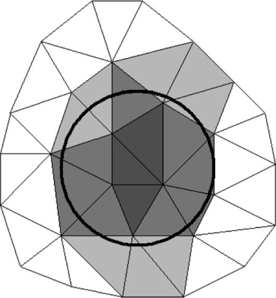
The calculations unit contains all the solving routines, its input being the setup files prepared by the GUI unit. The transport and reaction formulation is implemented using the long-established Finite Element Method (FEM).[29] For this, it uses OFELI (Object Finite Element Library)[30] to create the FEM mesh, interpret the user requirements and solve the model equations. The model space is subdivided into a large number of small parts to discretise the continuous volume. Each of these parts is considered to be homogeneous. These parts are called elements and together they form a mesh. Every element is identified by its nodes – points in space stored in the form of a vector (or array) of numbers. For microniches, elements are identified as being inside or outside the niche. Fig. 1 illustrates the equivalent 2-D situation. In 3-D, the circle becomes a sphere and the triangles become tetrahedrons. By increasing the mesh size, elements become smaller, leading to better spherical definition. Spatial resolution is set by specifying a value that controls the number of nodes per volume unit: the calculation precision improves as this number decreases. As an approximation, this value can be assumed to be the minimum linear resolution resolved by the mesh. For example, if the resolution is set at 0.05 (and the domain dimensions are in cm), the linear resolution will be at least as good as 500 μm (explained more fully in the Accessory publication). Further descriptions of mesh, model implementation and of more advanced features for the specification of microniches are provided as an Accessory publication.
|
Model inputs and calculations
The simulated system can be defined using the GUI, which allows the following input of data:
-
Initial vertical concentration profiles and concentrations within microniches for all chemical components.
-
Diffusion coefficients in water for each component separately.
-
Porosity – allows calculation of effective diffusion coefficients at each depth and for each microniche.
-
Selection of tortuosity equation – selects equation and variable values to be applied to the diffusion coefficient calculation.
-
Nature of the boundary for solute components – boundaries can be specified at the top and bottom of the domain.
-
Domain – input of domain dimensions, mesh resolution, model simulation run-time and calculation time-step.
-
Reaction stoichiometry, rates, and priorities.
With these data, all the possible components that are in the simulated system are specified. Each individual pool of OM is considered as a separate component, which effectively provides a very flexible multi-G model.[31–33] The multi-G approach is particularly suitable for this model, which considers sufficiently short periods of diagenesis that accumulation and burial processes can be disregarded. For other models where longer-term processes are considered, the power model (‘continuous-G’) of Middelburg[34] may be equally valid. Ultimately, knowledge of the behaviour and distributions of microbial communities and the degradation of known organic molecules and functional groups may lead to a more advanced understanding of OM degradation. However, given the current status of our understanding, the more holistic approach of multi-G is the best available option.
All the reactive species participate in reactions that each have a set of user-specified values: (a) priority group and order within this group (i.e. for OM pools and the order of oxidant utilisation); (b) reference component and concentration threshold (for specification of oxidants in OM reactions); (c) reaction rate constant (with specification to which reactant it is related, i.e. OM in case of OM decomposition reactions, or all components for secondary reactions); (d) type of reaction kinetics (zero or first order); (e) chemical equation of the reaction (stoichiometric values).
To calculate the effective reaction rate for a first order reaction, we use the following formula (Eqn 1):

where Re is the effective reaction rate, [Cspec] is the concentration of the appropriate component, RC is the reaction rate constant and Ψ accounts for the effect of porosity, φ, on the rate, by adjusting to concentration in unit volume of sediment. These porosity adjustments are specified according to Berg et al.[3]
As porosity can be specified as both a vertical profile and separately for microniches, Ψ introduces variations in the reaction rates with depth and within microniches (Eqn 2). Transformation reactions are included in the model for processes involving single species, for example reactive iron oxides converting into a form not reactive to OM[3] or the adsorption of a solute onto a solid phase.
There are two main types of reactions: primary and secondary. The difference between them lies in regulation of their execution, which follow the principles used by Hunter et al.[35] and Berg et al.[3]
Organic matter (involved only in primary reactions) can be defined as a series of separate components, each with their individual concentration profiles and distributions of microniches. A set of electron acceptors (EA; solutes or solids) facilitates the decomposition of each component of OM through a set of j primary reactions. Each reaction is assigned a priority index. When the concentration of the highest priority EA is above a prescribed threshold concentration [EA]lim, it is the only EA that reacts. The EA with the next highest priority can only be used when the concentration falls below [EA]lim. Each fraction of OM is consumed at a single prescribed rate that is first order with respect to OM, irrespective of the participating EAs. When [EA] < [EA]lim, the reaction still proceeds provided [EA] > 0, but its rate then becomes proportional to [EA], so that the primary redox reaction of OM degradation no longer follows a first-order process. This complex system of priorities and rates was implemented in the model by calculating the fraction, fi, of electrons consumed by the jth primary reaction using the elegant formula of Hunter et al.[35] (Eqn 3):
P is the number of primary reactions in a group. [EAj] is the concentration and [EAj]lim is the limiting (threshold) concentration of the reference component. If overlap of OM decomposition by two or more EAs is undesirable, the EA limiting concentrations can be set to a very low number (this avoids dividing by zero). Other reactions, which do not involve OM, are considered secondary and are allowed to proceed simultaneously at each timestep of the calculation according to their specified rate. Secondary reactions are considered to proceed with first order kinetics with respect to each component. However, the model retains the flexibility to specify overall first order (for a chosen component) or zero order, if required.
The reactive transport equation for the ith (mobile) aqueous component is shown in Eqn 4.
where Ci is the total aqueous concentration, Rreac,i is a source or sink rate due to chemical reaction, Di is the diffusivity coefficient (matrix) and vi is the porewater velocity vector of the ith component. Given the model does not consider advection (vi = 0), transport of the ith component is driven by reaction and diffusion processes only (Eqn 5)[36,37]:
The diffusion coefficient (Di) at a particular point is calculated from Eqn 6:
where D0 is the diffusion coefficient in water, θ is the tortuosity and φ is the porosity. A description of tortuosity and the various relationships built into the model are provided in the Accessory publication.
There are six boundaries in the modelled domain and, with the focus on small-scale features, the simulated volume will not necessarily encompass all diagenetic regimes. Boundary conditions can only be specified for solute species. Where upper or lower boundary concentrations are specified, they are considered to be Dirichlet boundaries (i.e. fixed concentrations) by the transport process solver. There are four options for specifying solute boundaries: only upper or lower boundary specified, both boundaries specified or no boundaries specified (this option assumes zero flux at the boundary, so that the gradients of concentration are equal to zero). Specified boundaries are defined by fixed concentrations entered by the user. Boundary conditions cannot be individually specified for the four sides of the domain (zero flux applies).
The top interface is commonly the surface of the diffusive boundary layer, where fixed concentrations that are representative of values in the overlying water are appropriate. The bottom interface does not have such a simple conceptual analogue. It is necessary because all solutes may not be generated by the model if a small vertical zone is being simulated to accommodate limited computing power. For example, if maxima in dissolved iron or manganese concentrations were expected to occur in the sediment considered, but below the depth included in the simulation, there would be an upward flux of solute iron and manganese, which would be oxidised within the modelled zone. In this case, a lower boundary condition with fixed concentrations of Fe and Mn can be specified, allowing inclusion of the solute flux due to processes outside the modelled domain.
The functionality of the OFELI software (diffusion process) has been verified independently by a large user base. Validation of all the reaction mechanisms was achieved by comparing outputs with known solutions. For example, to test both the OM oxidation reaction (which includes variables for porosity, time-step and [OM]) and the proper functioning of the limiting concentrations requires initial profiles for two or more oxidants, with the highest-order oxidant being allowed to drop below the limiting concentration. Consider a case where: (a) oxygen is present at the interface, but is quickly depleted; (b) manganese oxides are present equally throughout the domain, but below the limiting concentration; and (c) iron oxides are present equally throughout the domain and are above the limiting concentration. If OM is present at equal concentrations throughout the domain and the degradation rate is equal for all three oxidants, then the reduction in concentration of OM should be equal and predictable for all areas of the domain. By specifying a solid phase (immobile) product for each reactant, the consumption of reactants and generation of products can be calculated manually for each reaction using Eqns 1 to 3 and the reaction stoichiometry. Agreement of these calculations with modelled values provided verification of the framework for the primary metabolic pathways (see Accessory publication for a more explicit example).
Modelling solute dynamics at microniches of varying size
To demonstrate the capabilities of the model and to provide some insight into why microniche processes may be important, this section quantitatively investigates the effect of microniche size on solute distributions and the nature of the sulfide release from these hypothetical microniches. Previous modelling of microniches, as detailed in the introduction, has tended to investigate a limited number of components (O2, NO3–, N2) in one or two dimensions.[14,15,38] Investigations into the behaviour of marine snow microniches have been similarly limited,[28,39] although sulfide production in these environments has been measured.[40]
Here we sought to extend the pioneering work of Jørgensen[14] to model, in 3-D, multiple components at a microniche within an appropriate diagenetic framework. The modelling structure is largely based on a comprehensive dataset for a Danish marine sediment compiled by Fossing et al.[41] As data for microniches is limited, selecting input data for the model is not trivial. Assumptions about the ambient conditions and reaction priorities are required. Here we set reaction rates, starting concentrations and boundary concentrations to those modelled in 1-D by Fossing et al.[41] Within a simple 1-D description based on horizontally averaged sediment, overlap in redox zones is likely to be due to the heterogeneity of the sediment rather than specific biogeochemical controls occurring at given limiting concentrations. However, within a microniche, it may be more reasonable to assume that there will tend to be a dominant process at all times. This situation was recognised by setting limiting concentrations for oxidants of the bulk OM outside the microniche to those values used by Fossing et al.[41] The limiting concentrations for the oxidants of the OM within the microniche were set much lower (2% of the values of Fossing et al.[41]). Use of lower thresholds recognises that a single oxidant is likely to be largely responsible for OM degradation at discrete sites, while also accounting for both the likelihood that oxidant concentrations will become limiting before reaching zero and observations that microbial OM reducers utilising different EAs can coexist in the same locality (e.g. sulfate reduction and methanogenesis).[42] We also assumed that resupply or removal of porewater FeII and MnII from or to the solid phase is sufficient to buffer porewater concentrations for the 24 h modelled (these porewater concentrations were fixed for this modelling). OM microniches were assumed to contain negligible concentrations of metal oxides. Therefore, the only OM-oxidising components within the microniches were in solution, and oxidation followed the progression of O2, NO3–, SO42–. Microniche OM concentration was set at ~4–5 times the ambient OM concentration, consistent with observations by Kristensen and Pilgaard.[43] Rates for OM degradation were based on the multi-G-based data of Fossing et al.,[41] with the bulk OM degradation rates based on the slow-reacting phase (with rate kom-s) and the microniche rates based on the fast-reacting OM pool (with rate kom-f). The ratio of the rates (kom-f : kom-s) was 800. This rate results in the microniche OM concentration being depleted by ~12% of the initial value over the period modelled; one-third of the initial value will be reached after ~200 h. Initial profiles and tables of input parameters and reactions are provided in the Accessory publication.
With the input parameters described above and a domain of maximum x, y, z, dimensions of 0.6 × 0.6 × 1.05 cm, microniches of varying diameters were introduced at a depth of 0.25 cm below the sediment–water interface at the x, y coordinates of the centre of the domain. Given that the oxygen and nitrate penetration depths (defined here as the depth where the microniche limiting concentration is reached) in the absence of microniches are 0.26 and 0.67 mm respectively, the microniches have the potential to affect the profiles of multiple solutes. The largest niche has an upper edge at the sediment–water interface.
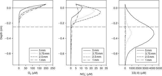
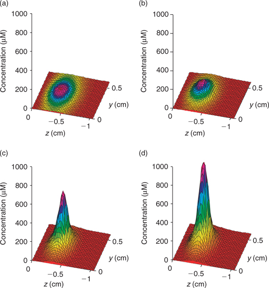
The 3-D distribution of solutes at four spherical microniches, of diameters 5, 3.75, 2.5 and 1 mm, was modelled. Fig. 2 shows the porewater profiles for O2, NO3–, and total sulfide (sum of S2–, HS– and H2S, referred to from this point as ΣS(-II)) through the centre of the microniches. The smaller niches (≤2.5 mm) have NO3– minima (barely discernible in the figure) centred within the niche. The slightly higher values below the niche centre are due to lateral diffusion, which would not be observed using a 1-D model. A NO3– maximum is created at the sediment surface by the intermediate-sized niche (2.5 mm). High sulfide concentrations are observed at the largest niches, with only limited sulfate reduction in the 2.5-mm niche and no sulfate reduction in the 1-mm niche where nitrate is not completely exhausted. Clearly the local geochemistry is very dependent on the size of any aggregate of OM. It will also be dependent on location. At greater depths where nitrate is absent, sulfide would be expected to be produced in small microniches, as observed by Widerlund and Davison.[12]
|
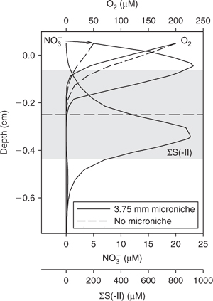
The significant localised changes in solute profiles that can be induced by the presence of microniches is further illustrated by Fig. 3, which shows the profiles for all three solutes arising from a 3.75-mm-diameter niche. The existence of sulfidic microniches in otherwise non-sulfidic zones of the sediment may have implications for the formation of metal sulfides. Trace metal sulfides are used as paleoredox proxies. Removal of metals from solution in sediments, where no removal is expected according to bulk data, may complicate interpretation of such paleodata.[13] Measurements of metals in porewaters at sulfidic microniches, using DGT, have shown that there may be localised supersaturation with respect to metal sulfides.[11]
|
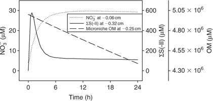
Time series data can be obtained from 3-D TREAD, as shown in Fig. 4, for NO3– and ΣS(-II) profiles at the 2.5-mm microniche over the first 24 h of the model run. Sulfide rapidly increases as the initial NO3– concentration within the niche is limited. As more NO3– is produced within the oxic sediment layer (owing to oxidation of ammonia released from the niche as OM is oxidised), less of the OM in the niche is oxidised by sulfate and the peak reduces to a plateau where a balance is achieved between NO3– production and loss. We recognise that this ammonia release may to some extent be retarded via uptake by the OM-oxidising bacteria, as depletions in porewater nutrients (phosphate) at microniches has been observed.[13] Fig. 5 graphically represents a plane of the 3-D data that can be produced from the model output. It shows how the magnitude of the concentration in a 2-D image is very dependent on how close the plane is to the centre of the microniche. Data from the present study corroborate the hypothesis of Brandes and Devol[15] that microniches may influence the general porewater chemistry of sediments via diffusion extending away from the discrete sites.
|
|
Conclusions
We have developed a model that considers reactions and transport occurring in 3-D within a sediment. Its graphical user interface allows it to be used by geochemists without expert modelling skills. Flexibility in the specification of reactions and the priority with which they occur facilitates detailed diagenetic modelling using a wide range of solutes and solid phases. Spherical microniches, where different rates and concentrations produce a localised chemistry, may be specified. The model has been tested by separately verifying individual reaction types. Modelling of the hypothetical cases of microniches in the near-surface sediment showed that, for the conditions selected, sulfide was readily generated, provided the microniche diameter was greater than 1 mm.
Acknowledgements
We thank members of the European Union (EU) TREAD Program for early input in model development and the EU for financial support. A. Stockdale was supported by the UK Natural Environment Research Council (NER/S/A/2005/13679).
Further details of model implementation and additional Tables and Figures. This material is provided as an Accessory publication on the journal’s website.
[1]
B. P. Boudreau ,
A method-of-lines code for carbon and nutrient diagenesis.
Comput. Geosci. 1996
, 22, 479.
| Crossref | GoogleScholarGoogle Scholar |
[Verified 14 January 2007]
[31]
B. B. Jørgensen ,
A comparison of methods for the quantification of bacterial sulphate reduction in coastal marine sediments. III. Estimation from chemical and bacteriological field data.
Geomicrobiol. J. 1978
, 1, 49.

[32]
[33]
J. T. Westrich ,
R. A. Berner ,
The role of sedimentary organic-matter in bacterial sulfate reduction – the G model tested.
Limnol. Oceanogr. 1984
, 29, 236.
[34]
J. J. Middelburg ,
A simple rate model for organic matter decomposition in marine sediments.
Geochim. Cosmochim. Acta 1989
, 53, 1577.
| Crossref | GoogleScholarGoogle Scholar |
[35]
K. S. Hunter ,
Y. F. Wang ,
P. Van Cappellen ,
Kinetic modeling of microbially-driven redox chemistry of subsurface environments: coupling transport, microbial metabolism and geochemistry.
J. Hydrol. 1998
, 209, 53.
| Crossref | GoogleScholarGoogle Scholar |
[36]
G. T. Yeh ,
V. S. Tripathi ,
A critical evaluation of recent developments in hydrogeochemical transport models of reactive multichemical components.
Water Resour. Res. 1989
, 25, 93.
| Crossref | GoogleScholarGoogle Scholar |
[37]
P. Engesgaard ,
K. L. Kipp ,
A geochemical transport model for redox-controlled movement of mineral fronts in groundwater flow systems: a case of nitrate removal by oxidation of pyrite.
Water Resour. Res. 1992
, 28, 2829.
| Crossref | GoogleScholarGoogle Scholar |
[38]
R. Jahnke ,
A model of microenvironments in deep-sea sediments: formation and effects on porewater profiles.
Limnol. Oceanogr. 1985
, 30, 956.
[39]
H. Ploug ,
M. Kühl ,
B. Buchholz-Cleven ,
B. B. Jørgensen ,
Anoxic aggregates – an ephemeral phenomenon in the pelagic environment?
Aquat. Microb. Ecol. 1997
, 13, 285.
| Crossref | GoogleScholarGoogle Scholar |
[40]
A. L. Shanks ,
M. L. Reeder ,
Reducing microzones and sulfide production in marine snow.
Mar. Ecol. Prog. Ser. 1993
, 96, 43.
| Crossref | GoogleScholarGoogle Scholar |
[41]
[42]
E. Senior ,
E. B. Lindström ,
I. M. Banat ,
D. B. Nedwell ,
Sulfate reduction and methanogenesis in the sediment of a saltmarsh on the east coast of the United Kingdom.
Appl. Environ. Microbiol. 1982
, 43, 987.
| PubMed |
[43]
Accessory publication