

Evidence for marine production of monoterpenes
Noureddine Yassaa A B , Ilka Peeken C D , Eckart Zöllner C , Katrin Bluhm C , Steve Arnold E , Dominick Spracklen E and Jonathan Williams A FA Air Chemistry Department, Max Planck Institute for Chemistry, D-55020 Mainz, Germany.
B Faculty of Chemistry, University of Sciences and Technology Houari Boumediene (U.S.T.H.B.), Bab-Ezzouar, 16111 Algiers, Algeria.
C Leibniz Institute of Marine Sciences at the University of Kiel (IFM GEOMAR), Biological Oceanography, D-24105 Kiel, Germany.
D Present address: Center for Marine Environmental Sciences MARUM, Bremen, Germany, and Alfred Wegener Institute of Polar and Marine Research, D-27570 Bremerhaven, Germany.
E Institute for Climate and Atmospheric Science, Environment Building, School of Earth and Environment, University of Leeds, Leeds, LS2 9JT, United Kingdom.
F Corresponding author. Email: williams@mpch-mainz.mpg.de
Environmental Chemistry 5(6) 391-401 https://doi.org/10.1071/EN08047
Submitted: 7 August 2008 Accepted: 5 November 2008 Published: 18 December 2008
Environmental context. Laboratory incubation experiments and shipboard measurements in the Southern Atlantic Ocean have provided the first evidence for marine production of monoterpenes. Nine marine phytoplankton monocultures were investigated using a GC-MS equipped with an enantiomerically-selective column and found to emit monoterpenes including (–)-/(+)-pinene, limonene and p-ocimene, all of which were previously thought to be exclusively of terrestrial origin. Maximum levels of 100–200 pptv total monoterpenes were encountered when the ship crossed an active phytoplankton bloom.
Abstract. Laboratory incubation experiments and shipboard measurements on the Southern Atlantic Ocean have provided the first evidence for marine production of monoterpenes. Nine marine phytoplankton monocultures were investigated using a GC-MS equipped with an enantiomerically-selective column and found to emit at rates, expressed as nmol C10H16 (monoterpene) g [chlorophyll a]–1 day–1, from 0.3 nmol g [chlorophyll a]–1 day–1 for Skeletonema costatum and Emiliania huxleyi to 225.9 nmol g [chlorophyll a]–1 day–1 for Dunaliella tertiolecta. Nine monoterpenes were identified in the sample and not in the control, namely: (–)-/(+)-pinene, myrcene, (+)-camphene, (–)-sabinene, (+)-3-carene, (–)-pinene, (–)-limonene and p-ocimene. In addition, shipboard measurements of monoterpenes in air were made in January–March 2007, over the South Atlantic Ocean. Monoterpenes were detected in marine air sufficiently far from land as to exclude influence from terrestrial sources. Maximum levels of 100–200 pptv total monoterpenes were encountered when the ship crossed an active phytoplankton bloom, whereas in low chlorophyll regions monoterpenes were mostly below detection limit.
Additional keywords: algae, isoprene, organic trace gases, Southern Atlantic Ocean.
Introduction
Trace organic gas species play several important roles in the atmosphere, influencing ozone photochemistry and aerosol physics (see e.g. ref. [1] and references therein). Many terrestrial sources of such species have been characterised and quantified,[2–4] including anthropogenic emissions associated with the production and use of fossil fuels (e.g. alkanes, alkenes and aromatics), and biogenic emissions from trees and plants (e.g. isoprene and monoterpenes) (see e.g. ref. [4]). In comparison to these extensive terrestrial investigations, relatively little has been done to assess inputs from marine sources. This was in part because of the more limited accessibility, but also because of the perception from earlier oceanic alkane measurements that the ocean is a globally minor source of such species.[5] Recently, however, it has become apparent that the surface ocean can play an important role in the budgets of both organic trace gases and aerosols. For example, the surface ocean has been shown to be a massive reservoir for oxygenated organic species[1,6] and a recent study of marine aerosols at a coastal site in Ireland[7] showed that the organic fraction contributes significantly (63%) to the sub-micrometer particle mass of aerosols collected over the North Atlantic Ocean during phytoplankton bloom periods. These high-organic-fraction aerosols may be generated directly by bubble bursting at the organic-rich sea surface, or by the emission and subsequent oxidation of biogenic gases that produce semivolatile products and aerosol.
To date very little is known about secondary organic aerosol (SOA) formation from trace organic species released by marine biota. The main exception is dimethyl sulfide (DMS), which is known to be produced biogenically in the ocean[8,9] and yields the inorganic aerosol component sulfate upon complete oxidation in the atmosphere.[10,11] Isoprene, the strongest terrestrial biogenic emission, has also been observed as an oceanic emission[12] and in laboratory based studies of plankton.[13–17] Furthermore, it has also been shown to form aerosols over the tropical rainforest,[18] and more controversially suggested as the cause of cloud droplet radius changes in clouds that form directly over phytoplankton blooms.[19] Surprisingly, several trace gas compounds that are known to form secondary organic aerosol in the terrestrial environment such as monoterpenes (a diverse group of molecules made up of two isoprene units) (see e.g. refs [20–22]), have never been investigated as emissions from plankton. The natural world is known to use these specific volatile compounds to signal opportunity to insects, pathogens and pollinators alike, or serve as a chemical defence.[23,24] Most of these monoterpenes are chiral, and although in most atmospheric chemistry studies the (+)- and (–)-enantiomers are not resolved, and hence measured together, the individual enantiomers often have markedly different biological properties.[24]
Here we present new data obtained from laboratory cultures of nine phytoplankton species and from shipboard measurements conducted as part of the OOMPH (Organics over the Ocean Modifying Particles in both Hemispheres) summer cruise in the Southern Ocean. Monoterpenes were studied first in the emissions of nine marine phytoplankton species (Coccolithophorid: Emiliania huxleyi; Diatoms: Chaetoceros neogracilis, Ch. debilis, Phaeodactylum tricornutum, Skeletonema costatum and Fragilariopsis kerguelensis; Chlorophyte: Dunaliella tertiolecta; cyanobacteria: Synechococcus and Trichodesmium) and then in the atmosphere over the Southern Atlantic Ocean conducted in January–February 2007 (35°49′S, 20°22′E to 52°17′S, 67°73′W) and 1–25 March 2007 (from 53°10′S, 70°54′W to 20°9′S, 57°29′E). The first leg of the cruise was planned to coincide with the large-scale summer phytoplankton bloom that occurs in the Southern Atlantic Ocean.
Experimental
Incubation experiments
In January–February 2006 several phytoplankton cultures were incubated and their gas phase emissions investigated within laboratories at the Leibniz Institute of Marine Sciences at the University of Kiel (IFM-GEOMAR, Kiel, Germany). Over the course of the experiments, nine phytoplankton species were studied, namely: Coccolithophorids: Emiliania huxleyi CCMP 371; Diatoms: Chaetoceros neogracilis CCMP 1318, Chaetoceros debilis and Fragilariopsis kerguelensis both isolated during the Polarstern cruise ANTXXI-3 (EIFEX by L. Hoffmann, IFM-GEOMAR, Kiel and P. Assmy, AWI-Bremerhaven), Phaeodactylum tricornutum (Phaeo, originating from the Falkowski laboratory) and Skeletonema costatum (AWI-Helgoland-culture collection); Chlorophyte: Dunaliella tertiolecta (DUN, originating from the Falkowski laboratory); cyanobacteria: Synechococcus RCC40 and Trichodesmium IMS101. Synechococcus RCC40 was grown in PCR-Tu2-medium[25] and the nitrogen fixing cyanobacterium Trichodesmium IMS101 was kept in YBCII medium with no dissolved nitrogen source for growth.[26] All other species were grown in f/2-medium.[27,28]
The cultures chosen during this experiment represent various key species of important biogeochemical provinces. F. kergulensis is an endemic species in the Southern Ocean, and Ch. Debilis, although also isolated from the Southern Ocean, is known to build worldwide open ocean blooms. S. costatum on the other hand is a typical coastal bloom forming species, while Trichodesmium is a representative of the nitrogen fixers in the tropical and subtropical regions, an area usually also inhabited by the other cyanobacterium: Synechococcus. E. huxleyi usually succeeds natural diatom blooms.
For the incubation experiments, duplicate 250-mL glass bottles (Schott, Germany) fitted with Teflon caps (Bola, Germany) were constructed with three ports to which 1/4-inch (0.635-cm) Teflon tubing could be fixed and through which gas could be flushed for air sampling. A length of Teflon tubing connected a three port Teflon valve at the top of the bottle, to below the liquid surface in the incubation flask so that samples could be periodically drawn out without perturbing the experiment. Within each flask pair, one of the flasks was designated as a control and filled with the growth medium (100 mL) of each algae species, while the second was filled with the investigated algae species in their respective media. Each flask pair was placed in an incubator and the temperature (4°C and 20°C) and PAR maximum intensity (30 or 100 μE m–2 s–1) were chosen according to the natural habitat of the different cultures, particularly for diatom species characteristic of the Southern Ocean. The light was programmed to follow a ‘natural’ diurnal light cycle illuminating from 0600 to 1800 hours. To produce a natural light intensity variation, the Light Thermostat was programmed to vary from 0% at 0600 hours, to reach a maximum at noon and thereafter progressively decrease back to 0% at 1800 hours. Synthetic air was flushed continuously through both flasks at identical flow rates (100 mL min–1). Air samples were then collected both from the air stream before entering the flasks for air blanks, and also at the exit to determine the net trace gas production of the various species. The difference between the inlet and outlet concentrations was attributed to the biogenic emission (or uptake) of the investigated species if the same difference was not observed in the control flask. The aim of this study was to screen as many phytoplankton species as possible, therefore, there are no replicates for the various species. However, since each species was monitored up to two days, the data presented here are a mean of 16 measurements.
Air samples taken before and after the incubation flasks were collected through stainless steel, two-bed sampling cartridges (Carbograph I/Carbograph II; Markes International, Pontyclun, UK) at a flow rate of 100 mL min–1. Prior to air sampling, the sampling cartridges were cleaned with the Thermoconditioner TC-020 (Markes International, Pontyclun, UK) by purging with helium 6.0 (99.9999%, Messer-Griesheim, Germany) for 120 min at 350°C and 30 min at 380°C. For storage, the cartridges were sealed with brass caps with PTFE ferrules and put into an airtight metal container (Rotilabo, Carl Roth GmbH & Co, Karlsruhe, Germany). After sampling, the cartridges were stored in a separate airtight metal container for a maximum of 12 h. Shortly before the analysis, the brass caps were exchanged for DiffLok caps (Markes International, Pontyclun, UK).
The average emission rates (taken at an optimal light intensity for each species) of total monoterpenes expressed as nmol total C10H16 (monoterpene) g [chlorophyll a]–1 day–1 emitted by the nine phytoplankton species were calculated using the following formula:
Open ocean experiments
Description of OOMPH cruise
Between January and March 2007, comprehensive shipborne measurements of trace gases and aerosols were made while crossing the South Atlantic Ocean from South Africa to Chile and back as part of the OOMPH (Organics over the Ocean Modifying Particles in both Hemispheres) field experiment (www.atmosphere.mpg.de/enid/oomph). The research vessel Marion Dusfresne traversed regions of relatively low marine biological productivity in the mid- and South Atlantic, and a high productivity region of a natural phytoplankton bloom in the west. The first leg was conducted from 19 January to 5 February 2007, from Cape Town, South Africa to Punta Arenas, Chile and timed to coincide with the annual phytoplankton maximum in this region. The second leg took place between 1 and 25 March 2007, from Punta Arenas, Chile to La Reunion Island, France.
Air samples
A central, high flow inlet for several trace gas instruments was installed at the top of the ship’s foremast (18 m above sea level). Air was drawn rapidly (at ~7 L min–1) through a 1.27-cm outer diameter, 75 m-long shrouded Teflon line. The residence time in the line was estimated as ~1 min.
Using the same type of cartridges as used in the laboratory, and employing the same cleaning and storage procedures, more than 100 cartridges were sampled during the first leg of the OOMPH cruise, and on the second leg a further 100 samples were taken on-line with the gas chromatograph-mass spectrometer (GC-MS) system described below. The sampling flow rate through the cartridge was 50 mL min–1 and the sampling duration was 1 h so that a total volume of 3 L was sampled.
Analytical procedure
A GC-MS analysis system was used to analyse the cartridges from both the laboratory and shipborne samples. This consisted of an air concentrating autosampler, and a thermal desorber (Markes Int., Pontyclun, UK), coupled to a gas chromatograph (GC6890A, Agilent Technologies, CA, USA), itself linked to a Mass Selective Detector (MSD 5973 inert) from the same company. All pertinent analysis parameters are summarised in Table 1. Laboratory multipoint calibrations of the monoterpenes and isoprene showed good linearity within the concentration ranges measured. One-point calibrations of a commercial volatile organic compound (VOC) standard (Apel-Riemer, CT, USA) were carried out at two hourly intervals. Blanks were taken regularly and showed no significant levels for the compounds discussed. The total uncertainties were between 10 and 15% in both laboratory experiments and shipboard measurements. In the laboratory 1.5 L were sampled whereas at sea 3 L were collected. The detection limits ranged from 0.5 to 5 pptv depending on the species in the laboratory study, and from 1 to 5 pptv in the marine atmospheric measurements.

|
Pigment samples
For phytoplankton pigment analysis, approximately every 3 h, 1–2 L of water from the ships seawater line (7 m below the ship), were filtered through GF/F filters, which were stored at –80°C until they were analysed by high performance liquid chromatography (HPLC), details are described in Hoffmann et al.[29] The taxonomic structure of the phytoplankton communities was derived from photosynthetic pigment ratios using the CHEMTAX program[30] applying the input matrix of Veldhuis and Kraay.[31] The phytoplankton group composition is expressed in chlorophyll a concentrations.
Back-trajectory weighted chlorophyll a exposure
For the ambient data samples, it was attempted to relate the monoterpene emissions to chlorophyll a concentrations in the seawater. However, simply correlating in-situ chlorophyll and observed monoterpene abundance does not account for air mass exposure to potential upwind sources or sinks from the ship sampling position. Rather than in-situ chlorophyll, we therefore used a time-series of back-trajectory weighted chlorophyll a to provide an estimate of the biological footprint sampled by air masses during transport to the ship. Ten-day kinematic back-trajectories initialised from the ship’s position are calculated from 1.0125-degree resolution ECMWF meteorological fields using the OFFLINE trajectory model.[32] The trajectory arrival frequency is one per minute, and positions are stored every 6 h back along the trajectories. At each position along a back trajectory, concentrations of ocean chlorophyll a are taken from monthly mean global fields from Level-3 SeaWiFS daily binned observations provided by NASA/GSF/DAAC, degraded to 0.25-degree (~30 km) resolution. An average chlorophyll a exposure was then calculated along each back trajectory, to produce a time-series of average chlorophyll a air mass exposure along the ship track. The use of monthly mean chlorophyll fields is a limitation, since we cannot account for variation in ocean chlorophyll on shorter timescales. In addition, the trajectories do not account for small-scale wind variability and sub-grid transport processes that may be active in the marine lower atmosphere. However, over the remote oceans, in the absence of strong convection and turbulent mixing, we expect the resolved flow in the ECMWF model to be relatively representative of the large-scale flow. The average chlorophyll values thus calculated will also have some dependence on the output frequency used for the trajectories (here 6 h). However, by degrading the resolution of the global chlorophyll fields, we have effectively spatially averaged the chlorophyll values, removing much of the bias given by the specific overlap locations of each trajectory time point and the chlorophyll field.
Results and discussion
Emission of monoterpenes from phytoplankton
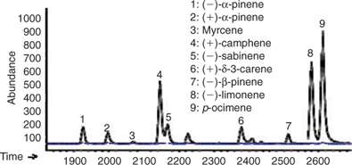
Among the nine marine phytoplankton monocultures investigated in this study, some cultures were found to have significantly enhanced levels of monoterpenes, while for others the monoterpene levels did not differ from the cultureless control. The monoterpenes were identified by combining mass spectroscopy data, elution order, and comparison of retention times of pure standards analysed under the same experimental conditions and following the analytical procedure described by Yassaa and Williams.[33] This is the first time monoterpenes have been identified as phytoplankton emissions.
Fig. 1 shows an example of the reconstructed mass chromatographic profile of monoterpenes obtained by analysing the gaseous emission of D. tertiolecta and the medium (overlayed in blue) on a β-cyclodextrin column using single ion mode (SIM). The chromatographic profile depicted in Fig. 1 was generated by plotting the current produced by ions with m/z 93, a fragment quite specific of monoterpene hydrocarbons that, in many cases, is the base peak of the mass spectrum. The numbers on the peaks refer to the identified compounds reported in Table 2. Nine monoterpenes were identified in the emission of D. tertiolecta; (–)- and (+)-α-pinene, myrcene, (+)-camphene, (–)-sabinene, (+)-δ-3-carene, (–)-β-pinene, (–)-limonene and p-ocimene. As reported in Table 2, p-ocimene accounted for 37% of the total monoterpenes and was the dominant measured monoterpene in the emission of D. tertiolecta. Since we have employed a β-cyclodextrin capillary separation column, the enantiomers of optically active monoterpenes were also well resolved. The average emission rates of the sum of monoterpenes expressed as nmol total C10H16 (monoterpene) g [chlorophyll a]–1 day–1 emitted by the nine phytoplankton species are reported in Table 3. Among the phytoplankton sampled, D. tertiolecta, a Chlorophycae species (close to 226 nmol g [chlorophyll a]–1 day–1), was the strongest emitter of monoterpenes followed by P. tricornutum (~68 nmol g [chlorophyll a]–1 day–1) and then by F. kerguelensis (~43 nmol g [chlorophyll a]–1 day–1). While D. tertiolecta is less important in oceanic phytoplankton, F. kerguelensis is an important, prolific species of the Southern Ocean, whose frustules make up most of the sediment in this region.
|
|
|
Since terrestrial vegetation is known to emit both isoprene and monoterpenes,[34] and it has been established that marine phytoplankton do emit isoprene,[12,17] the emission of monoterpenes from phytoplankton cannot be entirely unexpected. It is worth considering that terpenes are common metabolites in marine plants and their formation by the condensation of isopentenyl pyrophosphate units is, in this regard, comparable to terrestrial metabolism.[35,36] Unlike terrestrial biosynthesis mechanisms, marine terpene production is thought to involve halogens, particularly bromine, in the primary production of terpenes through cyclisation reactions. Bromine-induced cyclisation of a slightly modified monoterpene precursor yields a bromoterpene that can then be further halogenated. This process is common in marine organisms and a variety of haloterpenoids (~400 are known) can be produced.[35,36] There is no literature evidence of terrestrial emissions of haloterpenes, and likewise no evidence that marine phytoplankton or macroalgae produce monoterpenes with the same structures as found in terrestrial plants. However, myrcene was identified by Wise et al.[35] as a major monoterpene emission (32.6%) after (E)-10-bromomyrcene (33.2%) in cultured Ochtodes secundiramea tissue that was subjected to simultaneous steam distillation/solvent extraction and analysed by GC-MS. Previous measurements of various volatile organic compounds in ocean sediments[37] have also led the authors to speculate that marine terpenes may be precursors for biological and low temperature chemical formation mechanisms.
Shipboard measurements
Following the identification of monoterpenes in monoculture samples in the laboratory we sought to directly confirm this finding in ambient air. The Southern Atlantic is an ideal location to perform such measurements since there is practically no influence from advected anthropogenic pollution (in contrast to the North Atlantic) and a ship can be positioned so far from land that any short lived monoterpenes measured may be attributed to oceanic emissions.
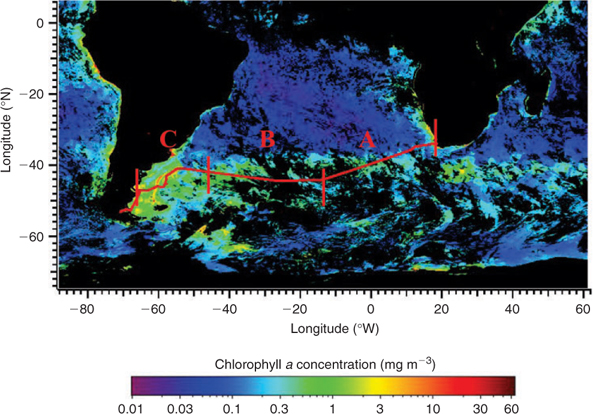
Fig. 2 shows a reconstructed mass chromatographic profile of monoterpenes in an ambient air sample collected over the Southern Atlantic Ocean at a position of 46°99′S, 64°70′W and at maximum monoterpene levels. Monoterpenes were positively identified following the procedure described above. It can be seen that monoterpenes were detected in remote marine air, consistent with an oceanic source of monoterpenes. However, in contrast to the monoculture experiments that showed p-ocimene as the dominant monoterpene emission, in the South Atlantic marine boundary layer (–)- and (+)-α-pinene were the major isoprenoid compounds in all samples. p-Ocimene and other monoterpene species were also identified, but at much lower levels. Therefore, only (–)- and (+)-α-pinene were quantified in this study. Table 4 reports the mixing ratios range of isoprene, (–)-α-pinene, and (+)-α-pinene, the sum of (–)-α-pinene and (+)-α-pinene, and the percent composition of (–)-α-pinene and (+)-α-pinene along with in-situ chlorophyll a and back-trajectory weighted chlorophyll a during the first leg of the cruise. The cruise can be divided into three regions according to the isoprene and α-pinene mixing ratios reported in Table 4. The first region was from 35°49′S, 20°22′E to 43°18′S, 11°17′W (denoted as ‘A’) where these organic species were at or close to the detection limit. The other two regions showed high concentrations, the first one termed ‘distant bloom (before reaching the bloom region)’ from 43°37′S, 11°76′W to 41°51′S, 48°42′W (denoted as ‘B’, from 25 to 31 January 2007 where the maximum α-pinene level was around 115 pptv); and the second one was termed ‘in-situ bloom’ from 41°51′S, 48°42′W to 47°55′S, 65°47′W (denoted as ‘C’, from 31 January to 3 February 2007 where the maximum α-pinene level was around 225 pptv).
|

|
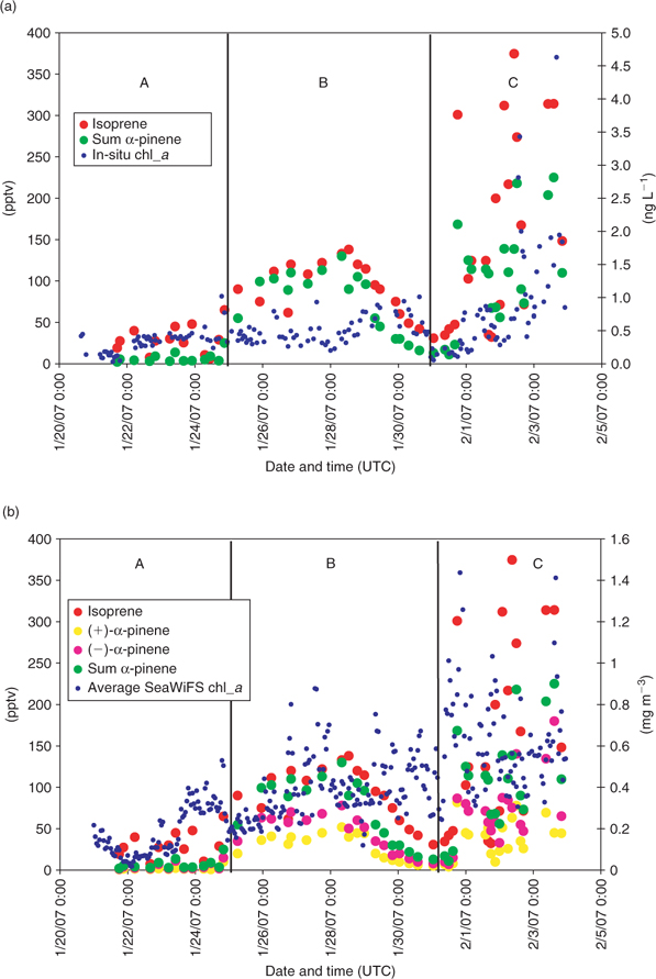
Fig. 3 shows that the vessel traversed regions of relatively low marine biological productivity in the mid- and South Atlantic (region A), and a high productivity region of a natural phytoplankton bloom in the west (region C). As mentioned in the previous section, in order to relate chlorophyll a and observed monoterpene abundance, we also used 10-day chlorophyll a weighted back trajectories, to provide an estimate of the biological footprint sampled by air masses during their transport to the ship. Fig. 4a, b depict the temporal variation of isoprene, (–)-α-pinene, (+)-α-pinene, and the sum of (–)- and (+)-α-pinene, along with in-situ chlorophyll a (calculated as the sum of divinyl-chlorophyll a and chlorophyll a) and 10-day back-trajectory weighted SeaWiFS chlorophyll a.
|
|
The pigment analysis showed that the areas were characterised by distinct phytoplankton compositions (Fig. 5). While in all regions, cyanobacteria built a solid background community, the low chlorophyll regions (region A) were also inhabited by a high proportion of prochlorophytes, typical for this oligotrophic region.[38] In the distant bloom area (region B), the relative proportion of green algae, namely the class of prasinophytes and chlorophytes, increased their relative distribution. D. tertiolecta, the profilic emitter of monoterpenes during the laboratory culture study, also belongs to the chlorophytes and thus, assuming that green algae and especially chlorophytes are strong monoterpene emitters, this might explain the increase observed in monoterpenes in this region. In the ‘in-situ bloom’ region (region C), the relative contribution of these groups decreases again, however, total chlorophyll has increased (Table 4), therefore, the actual concentration of this group is in the same range as before, which might explain the monoterpenes observed in region C. Since monoterpenes show the highest concentrations in this region, it is very likely that other groups in the bloom also contribute to this signal. Dinoflagellates and diatoms are dominant in some of the blooms indicated in Fig. 4a. Since dinoflagellates were not investigated in the laboratory study, we can only speculate that this group might also be a major monoterpene emitter. Another group, the pelagophytes, also not investigated during the laboratory studies, was important in region B and C and might also be responsible for some of the monoterpene emissions. Even though we are currently not able to pinpoint which group might be the most important monoterpene emitter in the field, a clear relation between the increase of phytoplankton and monoterpenes exists.

|
It is interesting to note that isoprene and α-pinene measured over the open ocean were correlated (r2 = 0.41), in particular within the bloom region (r2 = 0.57), which suggests that these two species have a similar emission source. In general, both isoprene and α-pinene appear to correlate with the 10-day averaged back-trajectory weighted chlorophyll a (see Fig. 4b), especially under the influence of the main phytoplankton ‘in-situ bloom’, again consistent with an oceanic phytoplankton-type source. It should be noted that a strong correlation between the simulated chlorophyll a values and the monoterpenes cannot be expected since phytoplankton speciation, chlorophyll content and well being (physiological state) vary greatly, and are likely to give rise to diverse monoterpene emission strengths. Moreover, the aforementioned laboratory study has highlighted the large variation in emission rates as a function of species. Furthermore, the weighted trajectories are necessarily based on monthly average chlorophyll distributions, which may differ slightly from the actual oceanic chlorophyll content encountered by the trajectories at specific times. From Fig. 4a, b and Table 4, it can be seen that with the 10-day averaged back-trajectory weighted chlorophyll a, the obtained correlation is better than with in-situ measured chlorophyll a. Closer inspection of Fig. 4b shows that the trajectories must have crossed a higher chlorophyll region of a ‘distant bloom’ some days before reaching the ship. This can be seen as two peaks that appear in the trajectory trace (the first one on 26 January around 1900 hours (UTC) and the second one on 27 January around 2200 hours (UTC)). The distant bloom region responsible for these peaks must have been emitting both isoprene and terpenes. Since the isoprene and monoterpene levels from the ‘distant bloom’ (region B) are only approximately two times smaller than those seen from the ‘in-situ’ bloom (region C) that we subsequently traversed, and come from a more distant region, we can argue, assuming similar wind speeds, that the more distant high chlorophyll region must have been a stronger emitter than the in-situ bloom. This is because some isoprene/monoterpenes will have been lost during the 3–4 days transport time as a result of oxidation by OH and O3.
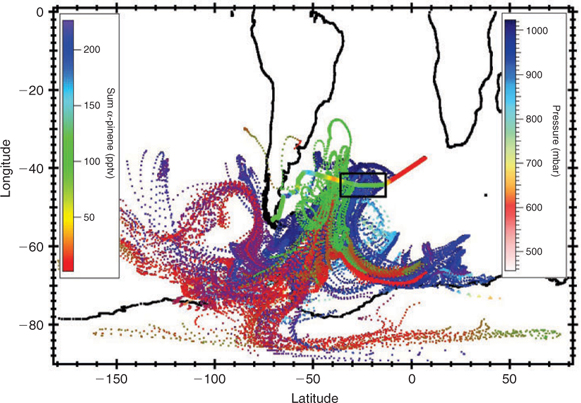
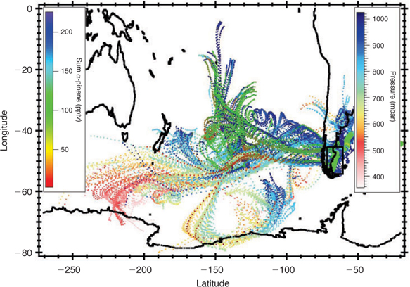
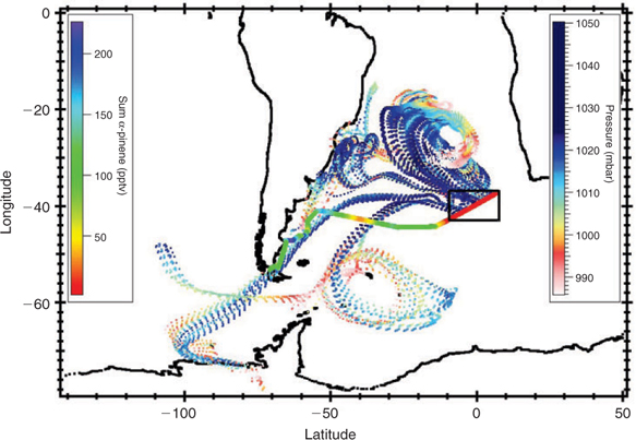
Since monoterpenes, and α-pinene in particular, are known to originate from terrestrial plants, we performed 10-day back-trajectories for the entire cruise track to determine the extent of land influence on the air samples. Figs 6 and 7 show the back-trajectories for the two regions of elevated monoterpene mixing ratios, respectively, while Fig. 8 represents the back-trajectories in a region where α-pinene was close to the detection limit. Both Figs 6 and 7 show that the sampled air masses were not influenced by continental influence in the past 10 days. Thus for land plants to have been responsible for the ~50 pptv monoterpenes observed over the ocean in the section highlighted in Fig. 6, the mixing ratios at source (over 10 days away) would have to have been in excess of 1 ppm, which is several orders of magnitude higher than any previously reported terrestrial measurements. This assumes an OH level of 5 × 10⁵ molecules cm–3 over the 10-day trajectory for α-pinene. We, therefore, conclude that the measured monoterpenes were most likely derived from ocean emissions.
|
|
|
Fig. 6 shows that the air masses in region B come predominantly from Antarctica. The high monoterpene and isoprene mixing ratios observed in the distant bloom region (zone ‘B’ in Fig. 4) may originate from diatoms living in sea ice in Antarctica or be emitted from regions between Antarctica and the ship. In any case we can exclude a terrestrial plant source. The back-trajectories displayed in Fig. 7 show that air masses traversing the main bloom (high chlorophyll region) originated from Antarctica and the Southern Pacific Ocean but passed over the southern part of South America before reaching the ship. In this case we cannot exclude an influence of terrestrial vegetation. Fig. 8 shows that although some back trajectories travelled near land, the α-pinene mixing ratios were still very low and close to the detection limit. This implies that either they were not influenced despite their proximity to land, or any terpenes emitted from this region have oxidised before reaching the ship. This presents further evidence that the monoterpenes observed over the open ocean were produced in-situ by marine phytoplankton and not influenced by terrestrial vegetation.
From the results of laboratory experiments and shipboard measurements we deduce that a suite of monoterpenes (including those identified in this work) are emitted by phytoplankton into the surrounding waters, and because of their low Henry Law coefficients, they are then emitted into the marine boundary layer air. It is not known whether such emissions simply leak through algal tissues or whether they are emitted as a response to biological (e.g. defence against predation) or mechanical (temperature, injury) stress.
Conclusions
Laboratory experiments and shipboard measurements over the Southern Atlantic Ocean have allowed the identification of marine monoterpene emissions for the first time. The phytoplankton emission rates of total monoterpenes were low and varied from 0.3 nmol g [chlorophyll a]–1 day–1 for S. costatum and E. huxleyi to 225.9 nmol g [chlorophyll a]–1 day–1 for D. tertiolecta. The maximum atmospheric monoterpene mixing ratios of 100–225 pptv were observed in the marine atmosphere of the Southern Atlantic Ocean in the region of one phytoplankton bloom where back trajectories show no land influence for the past 10 days.
These first results highlight the need for further studies on algae species in laboratory experiments and shipboard measurements to determine the levels and atmospheric impact of monoterpenes in other areas of the marine boundary layer. Even though the ambient air concentrations of monoterpenes are low, they may, because of their high reactivity, influence the photochemistry of the remote marine atmosphere. Small quantities of marine photochemically produced isoprene (a few pptv) have been shown to impact the formaldehyde budget at a remote coastal site in the southern hemisphere.[39] This is despite the estimated global marine source of isoprene (0.1 Tg year–1)[40] being dwarfed by the terrestrial source (~500 Tg year–1). Monoterpenes also form formaldehyde efficiently by photooxidation. However, the low levels of isoprene and monoterpenes measured here, namely over an order of magnitude less than terrestrial forested regions (see e.g. ref. [41]), indicate that the impact of marine monoterpene emissions on the formaldehyde budget will be small indeed. Nonetheless, in regions of high biological activity, e.g. the Southern Atlantic Ocean during the bloom period, such emissions could be of importance to local photochemistry. A further consideration is that the atmospheric oxidation products of these marine emissions, albeit minor in the absolute sense, may condense on existing aerosol and thereby change its physical properties such as reflectivity and hydroscopicity. Further investigations are needed to determine the potential effect of such higher molecular weight emissions from the ocean. Such studies should also determine possible driving factors for emission, such as ambient light, CO2 levels, temperature, growth stage, nutrient availability, and physiological and ecological state. Moreover, in future, marine ecosystem communities should also be investigated since zooplankton and bacteria may also influence emissions.
Acknowledgements
This work was completed as part of the OOMPH project (Specific Targeted Research Project (STREP) in the Global Change and Ecosystems Sub-Priority). SUSTDEV-2004-3.I.2.1. Project Number 018419. The authors are grateful for logistical support from the IPEV/Aerotrace program during the Southern Ocean cruise. The authors thank Tom Custer for his technical assistance during the laboratory experiments and the cruise and for making the back-trajectory figures, and Rolf Hofmann, Thomas Küpfel, Sarah Gebhardt, Vinayak Sinha and Aurélie Colomb for their technical assistance during the cruise.
[1]
J. Williams ,
Organic trace gases in the atmosphere: an overview.
Environ. Chem. 2004
, 1, 125.
| Crossref | GoogleScholarGoogle Scholar |
CAS |

[2]
A. Guenther ,
C. N. Hewitt ,
D. Erickson ,
R. Fall ,
C. Geron ,
T. Graedel ,
P. Harley ,
L. Klinger ,
et al. A global-model of natural volatile organic compound emissions.
J. Geophys. Res. 1995
, 100, 8873.
| Crossref | GoogleScholarGoogle Scholar |
CAS |
[3]
[4]
[5]
C. Plass-Dülmer ,
R. Koppmann ,
M. Ratte ,
J. Rudolph ,
Light nonmethane hydrocarbons in seawater.
Global Biogeochem. Cy. 1995
, 9, 79.
| Crossref | GoogleScholarGoogle Scholar |
[6]
H. B. Singh ,
A. Tabazadeh ,
M. J. Evans ,
B. D. Field ,
D. J. Jacob ,
G. Sachse ,
J. H. Crawford ,
R. Shetter ,
W. H. Brune ,
Oxygenated volatile organic chemicals in the oceans: interferences and implications based on atmospheric observations and air–sea flux exchange models.
Geophys. Res. Lett. 2003
, 30, 1862.
| Crossref | GoogleScholarGoogle Scholar |
[7]
C. D. O’Dowd ,
M. C. Facchini ,
F. Cavalli ,
D. Ceburnis ,
M. Mircea ,
S. Decesari ,
S. Fuzzi ,
Y. J. Yoon ,
J. P. Putaud ,
Biogenically driven organic contribution to marine aerosol.
Nature 2004
, 431, 676.
| Crossref | GoogleScholarGoogle Scholar |
CAS |
PubMed |
[8]
[9]
P. S. Liss ,
A. D. Hatton ,
G. Malin ,
P. D. Nightingale ,
S. M. Turner ,
Marine sulphur emissions.
Philos. Trans. R. Soc. Lond. B Biol. Sci. 1997
, 352, 159.
| Crossref | GoogleScholarGoogle Scholar |
CAS |
[10]
R. P. Kiene ,
T. S. Bates ,
Biological removal of dimethyl sulphide from seawater.
Nature 1990
, 345, 702.
| Crossref | GoogleScholarGoogle Scholar |
CAS |
[11]
R. P. Kiene ,
L. J. Linn ,
J. A. Bruton ,
New and important roles for DMSP in marine microbial communities.
J. Sea Res. 2000
, 43, 209.
| Crossref | GoogleScholarGoogle Scholar |
CAS |
[12]
B. Bonsang ,
C. Polle ,
G. Lambert ,
Evidence for marine production of isoprene.
Geophys. Res. Lett. 1992
, 19, 1129.
| Crossref | GoogleScholarGoogle Scholar |
CAS |
[13]
W. J. Broadgate ,
P. S. Liss ,
S. A. Penkett ,
Seasonal emissions of isoprene and other reactive hydrocarbon gases from the ocean.
Geophys. Res. Lett. 1997
, 24, 2675.
| Crossref | GoogleScholarGoogle Scholar |
CAS |
[14]
W. J. Broadgate ,
G. Malin ,
F. C. Kupper ,
A. Thompson ,
P. S. Liss ,
Isoprene and other non-methane hydrocarbons from seaweeds: a source of reactive hydrocarbons to the atmosphere.
Mar. Chem. 2004
, 88, 61.
| Crossref | GoogleScholarGoogle Scholar |
CAS |
[15]
P. J. Milne ,
D. D. Riemer ,
R. G. Zika ,
L. E. Brand ,
Measurement of vertical-distribution of isoprene in surface seawater, its chemical fate, and its emission from several phytoplankton monocultures.
Mar. Chem. 1995
, 48, 237.
| Crossref | GoogleScholarGoogle Scholar |
CAS |
[16]
R. M. Moore ,
D. E. Oram ,
S. A. Penkett ,
Production of isoprene by marine-phytoplankton cultures.
Geophys. Res. Lett. 1994
, 21, 2507.
| Crossref | GoogleScholarGoogle Scholar |
CAS |
[17]
S. L. Shaw ,
S. W. Chisholm ,
R. G. Prinn ,
Isoprene production by Prochlorococcus, a marine cyanobacterium, and other phytoplankton.
Mar. Chem. 2003
, 80, 227.
| Crossref | GoogleScholarGoogle Scholar |
CAS |
[18]
M. Claeys ,
B. Graham ,
G. Vas ,
W. Wang ,
R. Vermeylen ,
V. Pashynska ,
J. Cafmeyer ,
P. Guyon ,
M. O. Andreae ,
P. Artaxo ,
W. Maenhaut ,
Formation of secondary organic aerosols through photooxidation of isoprene.
Science 2004
, 303, 1173.
| Crossref | GoogleScholarGoogle Scholar |
CAS |
PubMed |
[19]
N. Meskhidze ,
A. Nenes ,
Phytoplankton and cloudiness over the Southern Ocean.
Science 2006
, 314, 1419.
| Crossref | GoogleScholarGoogle Scholar |
CAS |
PubMed |
[20]
J. H. Seinfeld ,
J. F. Pankow ,
Organic atmospheric particulate material.
Annu. Rev. Phys. Chem. 2003
, 54, 121.
| Crossref | GoogleScholarGoogle Scholar |
CAS |
PubMed |
[21]
M. Jaoui ,
R. M. Kamens ,
Mass balance of gaseous and particulate products from beta-pinene/O3/air in the absence of light and beta-pinene/NOx/air in the presence of natural sunlight.
J. Atmos. Chem. 2003
, 45, 101.
| Crossref | GoogleScholarGoogle Scholar |
CAS |
[22]
J. H. Kroll ,
Secondary organic aerosol formation from isoprene phtooxidation.
Environ. Sci. Technol. 2006
, 40, 1869.
| Crossref | GoogleScholarGoogle Scholar |
CAS |
PubMed |
[23]
R. Croteau ,
Biosynthesis and catabolism of monoterpenoids.
Chem. Rev. 1987
, 87, 929.
| Crossref | GoogleScholarGoogle Scholar |
CAS |
[24]
[25]
R. Rippka ,
T. Coursin ,
W. Hess ,
C. Lichtle ,
D. J. Scanlan ,
K. A. Palinska ,
I. Iteman ,
F. Partensky ,
J. Houmard ,
M. Herdman ,
Prochlorococcus marinus Chisholm et al. 1992 subsp pastoris subsp nov strain PCC 9511, the first axenic chlorophyll a2/b2-containing cyanobacterium (Oxyphotobacteria).
Int. J. Syst. Evol. Microbiol. 2000
, 50, 1833.
|
CAS |
PubMed |
[26]
Y. B. Chen ,
J. P. Zehr ,
M. Mellon ,
Growth and nitrogen fixation of the diazotrophic filamentous nonheterocystous cyanobacterium Trichodesmium sp IMS 101 in defined media: Evidence for a circadian rhythm.
J. Phycol. 1996
, 32, 916.
| Crossref | GoogleScholarGoogle Scholar |
[27]
[28]
R. R. L. Guillard ,
J. H. Ryther ,
Studies of marine planktonic diatoms. I. Cyclotella nana Hustedt and Detonula confervacea Cleve.
Can. J. Microbiol. 1962
, 8, 229.
|
CAS |
PubMed |
[29]
L. Hoffmann ,
I. Peeken ,
K. Lochte ,
P. Assmy ,
M. Veldhuis ,
Different reactions of Southern Ocean phytoplankton size classes to iron fertilization.
Limnol. Oceanogr. 2006
, 51, 1217.
|
CAS |
[30]
M. D. Mackey ,
D. J. Mackey ,
H. W. Higgings ,
S. W. Wright ,
‘CHEMTAX’ – a program for estimating class abundances from chemical markers: application to HPLC measurements of phytoplankton.
Mar. Ecol. Prog. Ser. 1996
, 144, 265.
| Crossref | GoogleScholarGoogle Scholar |
CAS |
[31]
M. J. W. Veldhuis ,
G. W. Kraay ,
Phytoplankton in the subtropical Atlantic Ocean; towards a better understanding of biomass and composition.
Deep-Sea Res. 2004
, I51, 507.
[32]
[33]
N. Yassaa ,
J. Williams ,
Analysis of enantiomeric and non-enantiomeric monoterpenes in plant emissions using portable dynamic air sampling/solid-phase microextraction (PDAS-SPME) and chiral gas chromatography/mass spectrometry.
Atmos. Environ. 2005
, 39, 4875.
| Crossref | GoogleScholarGoogle Scholar |
CAS |
[34]
J. Williams ,
N. Yassaa ,
S. Bartenbach ,
J. Lelieveld ,
Mirror image hydrocarbons from Tropical and Boreal forests.
Atmos. Chem. Phys. 2007
, 7, 973.
|
CAS |
[35]
M. L. Wise ,
G. L. Rorrer ,
J. J. Polzin ,
R. Croteau ,
Biosynthesis of marine natural products: isolation and characterization of a myrcene synthase from cultured tissues of the marine red alga Ochtodes secundiramea.
Arch. Biochem. Biophys. 2002
, 400, 125.
| Crossref | GoogleScholarGoogle Scholar |
CAS |
PubMed |
[36]
M. L. Wise ,
Monoterpene biosynthesis in marine algae.
Phycologia 2003
, 42, 370.
[37]
J. M. Hunt ,
R. J. Miller ,
J. K. Whelan ,
Formation of C4–C7 hydrocarbons from bacterial degradation of naturally occurring terpenoids.
Nature 1980
, 288, 577.
| Crossref | GoogleScholarGoogle Scholar |
CAS |
[38]
M. V. Zubkov ,
M. A. Sleigh ,
P. H. Burkill ,
R. J. G. Leakey ,
Picoplankton community structure on the Atlantic Meridional Transect: a comparison between seasons.
Prog. Oceanogr. 2000
, 45, 369.
| Crossref | GoogleScholarGoogle Scholar |
[39]
A. C. Lewis ,
L. J. Carpenter ,
M. J. Pilling ,
Nonmethane hydrocarbons in Southern Ocean boundary layer air.
J. Geophys. Res. – Atmos 2001
, 106, 4987.
| Crossref | GoogleScholarGoogle Scholar |
CAS |
[40]
P. I. Palmer ,
S. L. Shaw ,
Quantifying global marine isoprene fluxes using MODIS chlorophyll observations.
Geophys. Res. Lett. 2005
, 32, L09805.
| Crossref | GoogleScholarGoogle Scholar |
[41]
J. Williams ,
U. Pöschl ,
P. J. Crutzen ,
A. Hansel ,
R. Holzinger ,
C. Warneke ,
W. Lindinger ,
J. Lelieveld ,
An atmospheric chemistry interpretation of mass scans obtained from a Proton Transfer Mass spectrometer flown over the tropical rainforest of Surinam.
J. Atmos. Chem. 2001
, 38, 133.
| Crossref | GoogleScholarGoogle Scholar |
CAS |