

A mass balance inventory of mercury in the Arctic Ocean
P. M. Outridge A E , R. W. Macdonald B E G , F. Wang C E , G. A. Stern D E and A. P. Dastoor FA Geological Survey of Canada, 601 Booth St, Ottawa, ON, K1A 0E8, Canada.
B Department of Fisheries and Oceans, Institute of Ocean Sciences, PO Box 6000, Sidney, BC, V8L 4B2, Canada.
C Department of Chemistry, University of Manitoba, Winnipeg, MB, R3T 2N2, Canada.
D Department of Fisheries and Oceans, Freshwater Institute, 501 University Crescent, Winnipeg, MB, R3T 2N6, Canada.
E Department of Environment and Geography, University of Manitoba, Winnipeg, MB, R3T 2N2, Canada.
F Air Quality Research Division, Science and Technology Branch, Environment Canada, 2121 Trans Canada Highway, Dorval, QC, H9P 1J3, Canada.
G Corresponding author. Email: robie.macdonald@dfo-mpo.gc.ca
Environmental Chemistry 5(2) 89-111 https://doi.org/10.1071/EN08002
Submitted: 21 December 2007 Accepted: 21 February 2008 Published: 17 April 2008
Environmental context. Mercury (Hg) occurs at high concentrations in Arctic marine wildlife, posing a possible health risk to northern peoples who use these animals for food. We find that although the dramatic Hg increases in Arctic Ocean animals since pre-industrial times can be explained by sustained small annual inputs, recent rapid increases probably cannot, because of the existing large oceanic Hg reservoir (the ‘flywheel’ effect). Climate change is a possible alternative force underpinning recent trends.
Abstract. The present mercury (Hg) mass balance was developed to gain insights into the sources, sinks and processes regulating biological Hg trends in the Arctic Ocean. Annual total Hg inputs (mainly wet deposition, coastal erosion, seawater import, and ‘excess’ deposition due to atmospheric Hg depletion events) are nearly in balance with outputs (mainly shelf sedimentation and seawater export), with a net 0.3% year–1 increase in total mass. Marine biota represent a small fraction of the ocean’s existing total Hg and methyl-Hg (MeHg) inventories. The inertia associated with these large non-biological reservoirs means that ‘bottom-up’ processes (control of bioavailable Hg concentrations by mass inputs or Hg speciation) are probably incapable of explaining recent biotic Hg trends, contrary to prevailing opinion. Instead, varying rates of bioaccumulation and trophic transfer from the abiotic MeHg reservoir may be key, and are susceptible to ecological, climatic and biogeochemical influences. Deep and sustained cuts to global anthropogenic Hg emissions are required to return biotic Hg levels to their natural state. However, because of mass inertia and the less dominant role of atmospheric inputs, the decline of seawater and biotic Hg concentrations in the Arctic Ocean will be more gradual than the rate of emission reduction and slower than in other oceans and freshwaters. Climate warming has likely already influenced Arctic Hg dynamics, with shrinking sea-ice cover one of the defining variables. Future warming will probably force more Hg out of the ocean’s euphotic zone through greater evasion to air and faster Hg sedimentation driven by higher primary productivity; these losses will be countered by enhanced inputs from coastal erosion and rivers.
Introduction
Mercury in the Arctic is a scientific and policy issue of long-standing and increasing interest, partly because of its human and wildlife health implications, and partly because of the widely held view that the Arctic is a ‘sink’ for global atmospheric Hg contamination.[ 1 ] The exposure of northern peoples to Hg is among the highest in the world in terms of blood and hair Hg concentrations, and is well above World Health Organisation guidelines in many communities.[ 1 , 2 ] This relatively high intake stems mainly from the inclusion in traditional northern diets of large amounts of marine mammal and fish flesh that contain surprisingly high Hg levels.[ 3 , 4 ] For example, in beluga (Delphinapterus leucas) sampled during subsistence hunts across the Canadian Arctic, total Hg concentrations in the edible tissues – liver, muktuk (skin) and muscle – ranged from ~0.2 to 100, 0.19 to 1.93 and 0.15 to 3.88 μg g–1 wet weight, respectively, with most samples well above the recommended dietary guideline for total Hg of 0.5 μg g–1 wet weight.[ 5 ] It is of particular concern that over 90% of the total Hg in fish and marine mammal muscle is monomethyl-Hg (MeHg), which is a known neurotoxin.[ 6 ]
Explaining why Hg levels are high in many Arctic aquatic species has proved to be an elusive goal of research over the last 20 years. At least in part, they reflect the entry of anthropogenic Hg into Arctic food chains during the 20th Century as evidenced by retrospective studies of animal and human hard tissues (teeth, hair, feathers). Pre-industrial Hg levels in species including beluga, ringed seals, seabirds, polar bears and humans were up to an order of magnitude lower than in modern specimens.[ 7 – 11 ] But how anthropogenic Hg has been, and is being, transported to the Arctic has not been comprehensively researched. The presumption in recent scientific assessments (e.g. refs [1,3]) is that anthropogenic Hg enters the Arctic almost entirely through atmospheric transport and deposition. The discovery of springtime atmospheric Hg depletion events (MDEs[ 12 ]), which are unique to polar regions, seemed to confirm this presumption by providing a mechanism by which anthropogenic Hg transported from the south in the atmosphere could be efficiently scavenged and lead to enhanced deposition of Hg to Arctic surface environments.[ 13 ]
In recent years, however, investigations into the fate of this deposited Hg have created uncertainty about the actual importance of MDEs, and of the atmosphere generally, as a key pathway for Hg entry into the Arctic. It is now known that on average more than half of the Hg deposited during each MDE is rapidly photoreduced and revolatilised back into the atmosphere,[ 14 – 17 ] while under some conditions MDEs result in no measurable increase in snow Hg concentrations.[ 16 , 18 ] Adding to the uncertainty are findings from two recent field studies of MDE Hg deposition and re-emission, which reported widely divergent net springtime fluxes ranging from 0.21 ± 0.07 μg m–2 in the sub-Arctic at Churchill, Manitoba,[ 15 ] to 26 μg m–2 in the High Arctic at Barrow, Alaska.[ 19 ] Based on well-constrained Arctic lake Hg mass balance studies, Fitzgerald et al.[ 20 ] calculated a net annual atmospheric flux for northern Alaska of only 2.8 ± 0.7 μg m–2 year–1, and a possible MDE contribution of ≤1.2 μg m–2 year–1, consistent with the lower MDE flux estimate at Churchill but not the higher value from Barrow. Without further investigation, it is unclear whether these differences are due to methodology, regional or temporal variations in deposition, or site-specific microclimatic factors, but clearly the uncertainty is significant in terms of mass inputs. The deposition rate at Churchill, if applied to the Arctic Ocean, would add negligible amounts of Hg to the mass already present in seawater.[ 15 ] A second reason to question the overall effect of atmospheric Hg and MDEs is that there is a dichotomy between the trends of Hg in Arctic biota and in the atmosphere. In the Canadian Arctic and west Greenland, many species exhibit significant Hg increases over recent decades,[ 3 ] whereas atmospheric monitoring since 1995 at Alert in northern Canada and other stations in southern Canada shows a stable or declining Hg trend.[ 21 ] Also, there is evidence that the elevated 20th-century accumulation of sedimentary Hg observed in many High Arctic lakes may be largely an artefact of higher aquatic primary productivity and Hg scavenging due to climate warming, implying that the increases in atmospheric Hg inputs calculated from these sediment studies have been significantly overestimated.[ 22 ] Further work needs to be done on the complete Hg cycle to clarify the overall impact of the atmosphere and other transport pathways on Hg levels and trends in Arctic biota and the environment.
One approach to achieving a more accurate understanding of contaminant transport to and cycling in the Arctic is to construct regional mass balance budgets, which allow routes of entry (sources) and exit (sinks) to be compared quantitatively (e.g. see the mass balance constructed for hexachlorocyclohexane in the Arctic Ocean[ 23 ]). Fluxes can then be set against inventories in abiotic and biotic compartments to assess residence times for contaminants and thereby project the effect of actions to curtail emissions. It is only from this perspective that the true importance of the atmosphere and other pathways can be gauged, and their possible impact on contaminants in biota can be assessed. The synthesis involved in constructing a mass balance also helps to identify priority areas for future research and provides insights for policy makers, as exemplified by an Hg inventory for the Mediterranean Sea.[ 24 ] Non-atmospheric pathways of Hg transport into the Arctic include ocean currents, river inflows and coastal erosion[ 23 ] but, until recently, scant attention has been paid to these alternative possibilities or to the dynamics of Hg within the ocean itself. However, these neglected pathways are the focus of recent research conducted in Canada under the auspices of the ‘ArcticNET’ Network of Centres of Excellence into Arctic Climate Change (www.arcticnet-ulaval.ca, accessed 16 March 2008). ArcticNET research and other recent literature now allow at least a first-order approximation of the Hg mass balance to be constructed for the Arctic Ocean; in some cases the flux and inventory estimates are more reliable than first-order because of the longevity and coverage of the datasets now available.
The goal of the present paper is to present the first mass balance study of Hg in the Arctic Ocean (defined in Fig. 1), utilising best-available data for inflows, outflows and total masses in abiotic and biotic compartments. We also report and incorporate new, previously unpublished data on total Hg in Arctic seawater. We focus on the ocean because human exposure to Hg in the Arctic occurs primarily through marine food-webs and, with few exceptions, the highest Hg levels occur in Arctic marine animals.[ 3 , 4 ] In the context of this mass balance, the following questions will be addressed:

|
-
What is the relative importance of atmospheric, oceanic, and terrestrial–riverine fluxes of total Hg into the Arctic Ocean?
-
How do these inputs compare with the standing mass of Hg in marine biota?
-
Which physical, geochemical or biological fulcrums are likely to exert most control over biological Hg levels in the ocean?
-
How sensitive are these fluxes and fulcrums to climate change, given a rapidly warming Arctic?
We also discuss, where appropriate, available information on MeHg. However, the absence of data for key parameters means that a corresponding MeHg budget cannot be derived at this time for the Arctic Ocean.
General description of mercury transport pathways
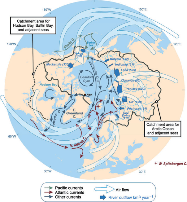
The hydrological, oceanographic and atmospheric circulation patterns and processes that transport Hg into the Arctic (see refs [23,25–27]) are briefly summarised here (Fig. 2). Water and sediment fluxes associated with these pathways are summarised in Tables 1 and 2.
|

|
|
Atmosphere
Tropospheric circulation patterns that bring airborne Hg from southern latitudes into the Arctic are influenced by low-pressure systems over the North Pacific (Aleutian Low) and North Atlantic (Icelandic Low) Oceans, and by high-pressure systems generally centred over Siberia and North America. Air masses originating in eastern North America and western Europe may enter the Arctic by the combined action of the Icelandic Low and North American High, which produce westerly winds over the North American continent and North Atlantic, and southerly winds over the Norwegian and Greenland Seas (see Fig. 2). The Siberian High, on its western side, tends to promote air movement into the Arctic from industrialised regions in eastern Europe and Siberia, whereas the Aleutian Low brings air from east Asia across the North Pacific and into Alaska, the Yukon and the Bering Sea. Interannual and decadal variability in these flow patterns is influenced by the Northern Annular Mode or Arctic Oscillation (AO), a robust, cyclical variation in atmospheric pressure gradients over the Arctic.[ 25 , 28 ] However, on average during winter, when the air pressure gradients are more intense than during summer and winds are therefore stronger and more consistently unidirectional, ~80% of the total south-to-north air transport into the Arctic is accounted for by these three pathways, i.e. southerlies over the Norwegian and Barents Seas (40%), eastern Europe and Siberia (15%), and the North Pacific Ocean and Bering Sea (25%).[ 28 , 29 ] In addition to direct transport of contaminants, AO-influenced wind patterns have an indirect effect on Hg transport by influencing the velocity and direction of surface ocean currents and sea-ice drift.[ 30 , 31 ]
Mercury is present in the atmosphere in different chemical forms that are subject to various rates of scavenging, deposition, and diffusion. Owing to its relatively high vapour pressure, low water solubility, and low reactivity, gaseous elemental mercury (GEM) has a relatively long tropospheric residence time of 6–24 months,[ 32 , 33 ] allowing it to be transported globally. The atmosphere also contains typically low concentrations of oxidised HgII species, operationally defined as reactive gaseous mercury (RGM; water-soluble HgII species with sufficiently high vapour pressure to exist in the gas phase) and particulate Hg (HgP; Hg II species that are adsorbed to atmospheric haze and dust particles).[ 34 ] Because of scavenging and surface adhesion processes, RGM and HgP have shorter atmospheric lifetimes (days to weeks[ 32 ]) than GEM, and are more readily deposited on local to regional scales.[ 35 ]
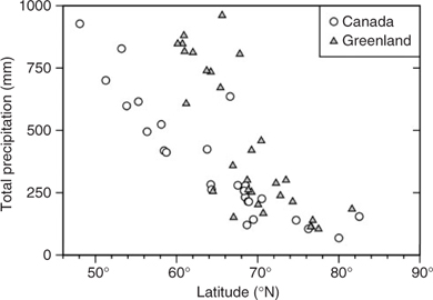
Once present in the Arctic atmosphere, Hg is subject to local deposition processes. These may include wet deposition, mainly of HgP scavenged by precipitation, and dry deposition of HgP and RGM. Precipitation as rain, snow or fog plays a major role in scavenging RGM and HgP from air at temperate latitudes,[ 36 ] but may be restricted by the desert-like conditions prevailing in the Arctic. There is a marked latitudinal pattern to total precipitation. In the Canadian and Greenlandic Arctic, for example, a more than three-fold decline in precipitation occurs from the sub-Arctic (south of 66°N) to ~80°N (Fig. 3). Thus, in the catchments of rivers flowing into the Arctic Ocean, which are mostly south of the Arctic Circle (see Fig. 2), precipitation rates are significantly higher than over the ocean itself. Average total annual precipitation for the Arctic Ocean is 340 mm, corresponding to 3300 km3 of water[ 27 ]; if long-term meteorological data for Alert (82.5°N, 62.2°W, on the edge of the Arctic Ocean) is a guide for our study area, then ~90% of the total falls as snow (measured as its rainfall equivalent, see www.msc.ec.gc.ca/climate/climate_normals, accessed 16 March 2008).
|
Wet and dry deposition of Hg occurs year-round in the Arctic. But after polar sunrise in spring, MDEs occur that act as a photochemical promoter of enhanced deposition,[ 13 ] converting substantial amounts of GEM into RGM and HgP that are then subject to wet and dry scavenging. GEM is usually the most abundant form of tropospheric Hg, with an Arctic baseline concentration of 1.5–1.8 ng m–3 [ 13 ] but can be depleted to <0.1 ng m–3 up to an altitude of ~1 km during MDEs.[ 12 , 37 ] Conversely, RGM and HgP concentrations in the Arctic troposphere are usually one to three orders of magnitude lower than that of GEM, but can dominate during and immediately after MDEs.[ 13 , 38 ] Kinetics studies indicate that halogens such as Br emitted from sea-ice are a necessary catalyst for MDEs and, correspondingly, transect studies report markedly higher Hg concentrations in snow deposited onto sea-ice and coastal areas compared with sites more than 25 km inland.[ 16 , 39 ] Thus, MDE deposition of Hg should be higher in the marginal Arctic seas than in the catchment areas of Arctic rivers.
Between 50 and 90% of the Hg deposited during winter and spring is rapidly revolatilised from snowpacks back to the atmosphere by photoreduction and GEM re-emission,[ 14 , 15 , 17 ] before it can enter aquatic and terrestrial environments. Indeed, one of the most important differences between Arctic and temperate regions in terms of atmospheric Hg dynamics may be tree cover, which provides shade to snowpacks under temperate forests and thereby greatly reduces the photoreduction and loss of deposited Hg.[ 40 ] For our purposes, we define re-emission as the volatilisation of Hg from snowpacks, from the first snowfall of winter to the end of spring snowmelt and runoff. Subsequently, volatilisation of GEM from the ocean can occur during summer and fall until sea-ice cover is re-established the following winter; this process is defined as evasion and is described below.
River and groundwater inflows
Rivers and groundwater transport Hg to the ocean in dissolved and particulate (suspended sediment) forms. Studies in sub-Arctic and temperate rivers show that Hg fluxes are correlated with flow and particulate organic carbon flux.[ 41 , 42 ] Although precipitation is higher over sub-Arctic catchment areas than over the Arctic Ocean, rivers flowing into the ocean are estimated to contribute the equivalent of only 212 mm of rainfall each year because evapotranspiration is also higher.[ 43 ] In our budget area (Fig. 1), this contribution yields an annual runoff of 3300 km3 (Table 1), with the Russian rivers Yenisey (620 km3), Lena (523 km3), and Ob (404 km3), and the Mackenzie River (330 km3) in Canada contributing the largest flows.[ 43 ] Interannual variability of total flow in Arctic rivers is ~30% of the mean based on discharge records from the 1920s onwards, although individual rivers can display larger variations.[ 43 , 44 ] Groundwater inflows are estimated to be <10% of total river discharge (294 km3 year–1 [ 45 ]). Stein and Macdonald[ 46 ] estimated the total sediment loading from rivers to the Arctic Ocean was 227 Mt annually, dominated by the Mackenzie (124 Mt), Lena (20.7 Mt) and Ob (15.5 Mt).[ 47 ]
Coastal erosion
Whereas the Mackenzie River is the dominant suspended sediment source to the Beaufort Sea, coastline erosion in northern Siberia is the major source to the East Siberian Sea.[ 46 ] Erosion rate varies significantly with coastal bluff height, coastal geology, ground ice content, and exposure. Current erosion losses in highly dynamic areas such as the Beaufort and Laptev Seas can be as much as several metres per year.[ 48 ] Total sediment flux from coastal erosion to the ocean is estimated at 430 Mt year–1.[ 46 ]
Ocean currents
The three main points for seawater exchange with the Arctic Ocean are the Bering Strait, Fram Strait and the Barents Sea, and the Canadian Arctic Archipelago (Fig. 2; Table 2). The Bering Strait is a broad, shallow (~50-m depth) sill over which on average 26 200 km3 of Pacific Ocean water flows into the Arctic annually.[ 49 ] On the Atlantic side, a greater net volume of water (110 400 km3) flows annually into the Arctic Ocean; however, because the salinity of Pacific water is less than that of the Atlantic, Pacific waters overlie the Atlantic Layer over about half of the Arctic Ocean area.[ 28 ] The northward penetration and vertical mixing of Atlantic waters is enhanced during periods of positive AO Index, which results in generally stronger southerly winds over the Barents and Greenland Seas. Nonetheless, there is a consistent net west-to-east movement of water through the Arctic Ocean from the Pacific to the Atlantic, which is driven by the pressure gradient created in part by salinity and temperature differences between the two oceans.[ 50 , 51 ] In terms of ocean currents that deliver Hg to Arctic marine food-webs, surface waters down to ~200 m are most important, as these are where most marine biota are found and where primary production occurs. Therefore, Hg in Pacific waters would be of greatest relevance in the western Arctic, whereas Hg from the Atlantic would be relevant to the eastern Arctic and to all deep water.[ 28 ] In terms of exchanges with the atmosphere and ice interactions, it is likely that the top 50 m of the water column is most important as this encompasses the polar mixed layer.[ 28 ] But for the present mass balance, seawater Hg data are not yet sufficiently refined to allocate the masses to these various zones.
Sedimentation
Sediment capture rates are well constrained for the Arctic Ocean, and are markedly higher on the ocean’s continental shelves (463 Mt year–1) than in the Central Basin (142 Mt year–1).[ 46 ] To balance sediment mass within the system, a small net export of 49 t year–1 in ocean currents has been added to Table 2, but has not been added as an extra line in our Hg budget calculations because we assume suspended sediment Hg will be captured in seawater total Hg values.
Evasion
Evasion of dissolved gaseous Hg (DGM) from seawater is an important component of the global Hg cycle, with an estimated net efflux of 1500 t year–1 (7.3 Mmol year–1).[ 52 ] Mercury transport across the air–seawater interface depends on the concentration gradient of GEM in the air and DGM in surface seawater, as well as environmental parameters that affect transfer velocity. Because the formation rate of DGM is dependant on microbial- and photoreduction of HgII, and because a cap of sea-ice would attenuate photoreduction and retard DGM exchange with air, polar regions are thought to exhibit globally insignificant rates of evasion.[ 53 ] However, it may be locally significant in the Arctic, especially from open waters such as polynyas and ice leads, and seasonally important over the shelves, which are now usually clear of ice during late summer. Seawater under the ice near Ellesmere Island contained DGM concentrations as high as 0.13 ± 0.04 ng L–1, suggesting that GEM efflux from open waters might be as much as 130 ± 30 ng m–2 day–1.[ 54 ] This calculated rate is similar to the maximum measured in the Mediterranean Sea,[ 55 ] and the Baltic Sea.[ 56 ] During the Polarstern research cruise in summer 2004, DGM supersaturation of seawater at latitudes above 74°N was reported, with DGM concentrations triple those in more southerly locations.[ 57 ] Like the Baltic[ 58 ] and other subpolar waters,[ 53 ] the Arctic Ocean may exhibit a seasonal reversal of GEM flux with significant evasion during spring and summer and a net influx during winter, although further work is required to prove that this is the case.
Sea-ice drift
Sea-ice is potentially an important transport mechanism for Hg within and out of the Arctic Ocean, either by the accumulation of atmospherically deposited Hg on ice or by the incorporation of shelf sediments through grounding or suspension freezing in shallow continental seas.[ 59 ] The Laptev and Kara Seas are the main sources of new ice within the Ocean’s Central Basin, and contribute significantly to the net yearly export of 2200–2500 km3 of ice (expressed as water volume) through Fram Strait,[ 27 , 60 ] which carries with it 8.6 Mt of sediment.[ 46 ]
Mass balance development
Calculation of mercury fluxes into and out of the Arctic Ocean
The following calculations refer to Hg fluxes into and out of the defined budget area, comprising 9.54 × 10⁶ km2 (Fig. 1; Table 1), which is almost identical to that used by Serreze et al.[ 27 ] for their freshwater mass balance. Table 3 summarises the Hg budget calculations. In general, best estimates were determined to be the median or mean values from individual studies, chosen on the basis of judgement about the adequacy (coverage and intensity) of sampling, internal consistency of data, and in some cases the capabilities of the research group concerned. The minimum and maximum fluxes determined for each parameter can be taken as a crude approximation of the uncertainty around each best estimate; however, these values can only be better constrained with additional empirical data.

|
Atmosphere
Atmospheric Hg fluxes include additions to the ocean from wet and dry deposition of RGM and HgP, and losses through re-emission and evasion of GEM. A range of modelled deposition estimates incorporating gross MDE-related flux has been published for variably defined areas of the Arctic. These ranged from 100 t year–1 for areas north of 70°N[ 37 ] to 325 t year–1 comprising 100 t year–1 from MDEs and 225 t year–1 from other processes.[ 61 ] Other figures fall within these limits (208 t year–1 for ‘the Arctic’,[ 62 ] and ~150–300 t year–1 in polar spring only[ 63 ]). None of these studies incorporated post-MDE re-emission or oceanic evasion in their calculations, nor were they constrained by actual flux measurements.
For the present review, a net deposition estimate incorporating the MDE effect on wet and dry deposition, as well as re-emission from snowpacks and evasion from the ocean, was determined using a modified Global/Regional Atmospheric Heavy Metals (GRAHM) model.[ 64 ] The model does not presently allow the MDE effect to be quantified separately from ‘baseline’ wet and dry deposition in spring (i.e. that not associated with MDEs), but expresses net deposition during spring separately from that in other seasons. For modelling the MDE effect, Br and BrO are considered as the most efficient reactants for oxidising Hg0 during MDEs.[ 61 , 65 , 66 ] Rate coefficients for the Hg0–Br reaction range from 1.1 × 10⁻¹² to 3.6 × 10⁻¹³ cm3 molecules–1 s–1,[ 67 ] which is one of the major sources of uncertainty in modelling atmospheric Hg cycling. Owing to this parameter alone, the uncertainty is ~6%; further information on uncertainties in the current generation of Hg deposition models is given by Lin et al.[ 68 , 69 ] The GRAHM version used for the present study includes halogen–Hg reaction rate coefficients based on Ariya et al., [ 61 ] which was selected on the basis of giving the best correlation between model-simulated MDEs and observed MDEs at Alert, Canada, over multiple years. Processes responsible for Br liberation in the Arctic boundary layer are not fully understood, but sea-salt aerosols, sea-salt deposits on snow, new sea-ice surfaces and frost flowers have been suggested as Br sources.[ 70 ] In the absence of a complete understanding, the model utilises GOME (Global Ozone Monitoring Experiment) satellite-derived monthly average BrO concentrations in the marine boundary layer. Present knowledge of Hg redox chemistry in snow is also limited for re-emission parameterisation. Thus, re-emission in the model is based on results from Poulain et al.[ 17 ] and Kirk et al. [ 15 ] and parameterised as a function of solar radiation reaching the surface including the influence of clouds and surface temperature. Model evasion for the Arctic Ocean is based on the global ocean estimate of 13 Mmol year–1,[ 52 ] and spatially distributed according to Hg deposition pattern and oceanic primary productivity (source: www.marine.rutgers.edu/opp, accessed 16 March 2008). Seasonal and diurnal dependence is added to evasion as a function of solar irradiance. The modified GRAHM model calculates a net atmospheric flux of 98 t year–1, which incorporates re-emission of 133 t year–1 and evasion of 12 t year–1 (thus, gross flux was 243 t year–1). Of the net flux, 46% (45 t) occurs during springtime, and 54% (53 t) at other times of the year.
An independent estimate of net atmospheric input, based on field measurements of parameters associated with atmospheric flux, is calculated here. Analogous to the GRAHM model, net annual atmospheric flux is calculated as:
For net winter and spring deposition, measurements of Hg in snowmelt runoff was employed. Mercury in snowmelt should reflect the integrated result of winter wet and dry deposition, the repeated springtime cycles of MDE-related and -unrelated deposition, and re-emission, because melting occurs after MDEs have ceased and photoreduction has acted on the Hg deposited in snowfall.[ 15 ] As Lindberg et al.[ 63 ] pointed out, meltwater is the logical first stage in the possible link between MDEs and Hg in Arctic biota. Mercury concentrations measured in snow meltwater across the Canadian and Greenland Arctic were between 0.3 and 10 ng L–1 (Fig. 4), with an average of ~3 ng L–1. The most comprehensive survey[ 15 ] sampled meltwater over sea-ice throughout the complete melt cycle for 2 consecutive years at Churchill, Manitoba, finding a mean of 4.0 ± 2.0 ng L–1. Assuming that 90% of total precipitation over the ocean occurred as snow (2960 km3; see above), and that all of the Hg remaining in sea-ice snowpacks was delivered to the ocean in the year of deposition, 3 ng L–1 in meltwater corresponds to a net winter–spring flux of 8.8 t.
|
Wet deposition during summer–autumn in the Arctic Ocean can be estimated from Hg measurements on precipitation collected at Churchill.[ 71 ] From July to October 2006, Hg concentrations in samples collected every two weeks averaged 9.3 ± 9.0 ng L–1 (rain, and snow as its water equivalent) with a total flux during this period of 1.0 μg m–2 and an uncertainty of ±0.1 μg m–2 calculated as the standard deviation of the fluxes of samples collected every two weeks. Churchill may be representative of a wide area of the Arctic. The total wet flux (June 2006 to June 2007) at Churchill was 1.4 μg m–2 year–1, which is similar to 1.5 μg m–2 year–1 in northern Alaska calculated from summer precipitation sampling,[ 20 ] and close to the minimum of 2.1 μg m–2 year–1 at remote sites in mid-continental North America (see www.nadp.sws.uiuc.edu/mdn, accessed 16 March 2008). Our estimate of 1.0 μg m–2 should be a maximum summer–autumn rate for the Arctic Ocean, because average precipitation is lower over the ocean (340 mm[ 27 ]) than the total at Churchill (456 mm) during the study period (see www.msc.ec.gc.ca/climate/climate_normals, accessed 16 March 2008). Scaling-up 1.0 μg m–2 to the budget area gives 9.5 t total Hg. An estimate of Hg in dry deposition during summer–autumn of 0.11 t can be derived from an aeolian dustfall of 5.7 Mt year–1,[ 46 ] pro rated to July to October, and an assumed concentration in Arctic airborne dust (taken as the average of 0.06 μg g–1 dry weight (DW) in uncontaminated soils[ 72 ]). Independently, Fitzgerald et al.[ 20 ] calculated dry Hg deposition in northern Alaska to be 0.1 μg m–2 year–1, corresponding to 0.3 t for summer–autumn for the Arctic Ocean. The total wet and dry deposition for summer–autumn for the ocean thus is (9.5 + 0.1) = 9.6 t.
The annual total atmospheric deposition incorporating re-emission but not evasion is therefore (9.6 + 8.8) = 18.4 t year–1. Evasion from the ocean was estimated in two ways. Field measurements of GEM and DGM were made during the Polarstern cruise in the North Atlantic and Arctic Oceans up to 84°N in summer 2004.[ 38 , 57 ] With an average GEM of 1.8 ng m–3 and DGM of 35 pg L–1 (average values for regions north of 74°N), and assuming an average windspeed at 10-m height, u10, to be 5 m s–1 and temperature of 1°C, evasion is calculated to be 6.4 μg m–2 year–1 over the open ocean. Assuming 5–20% of the Arctic Ocean is open on a yearly basis (D. Barber, University of Manitoba, pers. comm.), this amounts to a range of 3–12 t year–1 with an average of 7.5 t year–1. The second approach was based on the modelling of Strode et al.[ 53 ] who estimated a maximum evasion of ~50 ng m–2 month–1 or 0.6 μg m–2 year–1 for latitudes north of 70°N. Extrapolating to the Arctic Ocean produces an evasion of 5.7 t year–1. A figure of 10 t year–1 will be used in the mass balance.
Therefore, this field measurement-based approach results in an annual net atmospheric loading of (18.4 – 10) = 8.4 t year–1, over an order of magnitude lower than that provided by the GRAHM model. These values cannot be directly compared with previously published estimates because the latter do not include an evasion term. However, our earlier value of deposition without an evasion term (18.4 t year–1) is similar to the 23 t year–1 input calculated for the ‘High Arctic Ocean’ on the basis of snowpack sampling by Lu et al. [ 73 ] allowing for a pro rata adjustment to our budget area, and to a figure of 27 ± 7 t year–1 calculated from a net atmospheric flux of 2.8 ± 0.7 μg m–2 year–1 for lakes in northern Alaska.[ 20 ]
The two approaches explored here – modelling and field measurement – offer a stark choice for use in the Hg mass balance. Both have strengths and weaknesses; although the model needs to be constrained by actual field measurements, it pertains directly to the Arctic Ocean, whereas the field measurements are geographically narrowly focussed and must be extrapolated to the budget area. For this current budget, 98 t year–1 will be used as the best estimate for net atmospheric inputs because it is intermediate between earlier model values and the measurement-based estimates. As it is also the maximum reasonable estimate, its inclusion means that the influence of atmospheric inputs has been maximised in the resulting mass balance.
Oceans
Seawater Hg values contributing to ocean current fluxes were based on samples taken from sub-Arctic or temperate regions outside the defined area, whereas Hg data from inside the area were considered during calculation of standing mass in the abiotic ocean compartment (see below). Owing to the historical lack of attention given to the marine chemistry of Hg, reliable seawater data are sparse, and the mixture of filtered and unfiltered concentration data in the available literature[ 36 ] means that one cannot reliably quantify Hg in dissolved and suspended particulate forms. The limited data for mid-latitude surface waters suggests that particulate Hg is <5% (<0.01 ng L–1 [ 74 , 75 ]) of total Hg although the fraction may be higher in the Arctic Ocean. A median particulate Hg concentration of ~0.05 ng L–1 (range of 0.03–0.23 ng L–1) was reported from the Eurasian Arctic Ocean and the Barents Sea (calculated from [76]). Limited data from North Atlantic surface waters suggest that colloidal Hg (1000 Dalton molecular mass to 0.45-μm filter pore size) comprised ~25% of total Hg, and had a ~10-fold higher volume-based concentration than particulate Hg (>0.45 μm).[ 74 ] These colloidal forms were probably included in both filtered and unfiltered seawater data reported in the literature. For our purposes, we do not distinguish between dissolved and particulate Hg, but instead refer to ‘total’ seawater Hg concentrations. Surface water total Hg data considered during calculation of the oceanic inflows and outflows are summarised in Table 4, which also shows the minimum, maximum and best estimate values chosen for the mass balance.

|
Overall, most seawater total Hg concentrations lay in the range of 0.1 to 1.6 ng L–1, with higher values in the North Atlantic than the North Pacific. MeHg concentrations were usually <0.1 ng L–1 in Arctic Ocean outflow waters but comprised a surprisingly high proportion (30–45%) of total Hg.[ 54 ] By comparison, in South Atlantic surface waters, MeHg was <2% of total Hg.[ 75 ] For calculation of North Pacific Hg inputs to the Arctic Ocean, the median value of 0.15 ng L–1 from Laurier et al.[ 77 ] was used, with a range of 0.11 to 0.38 ng L–1 (Table 4). Given the small volume of inflow (Table 2), the best estimate Pacific contribution to the Arctic is 3.9 t year–1, which is an order of magnitude smaller than the North Atlantic contribution of 44.2 t year–1 based on a mean seawater Hg concentration of 0.40 ng L–1.[ 78 ] For calculation purposes, we have assumed outflows through the Canadian Archipelago and Fram Strait were equivalent to the inflows through the Bering Strait and the Barents Sea, respectively, plus a small additional outflow (3090 km3 year–1, divided between the two outlets) to account for freshwater inflows to the ocean. Best estimate concentrations of 0.50 and 0.48 ng L–1, respectively (Table 2), give Hg effluxes of 13.6 and 53.9 t year–1. Total seawater influxes and effluxes come to 48 and 68 t year–1, respectively. We assumed that the Hg mass in the net sediment outflow of 49 Mt year–1 is captured in total seawater data; even if a separate term was included, the additional efflux would be only ~5 t year–1 based on an average suspended sediment Hg concentration (0.1 μg g–1) like that of deep basin sediments.
Sea-ice
A single measurement of dissolved Hg in sea-ice of 0.8 ng L–1 [ 79 ] gives a 2.0 t year–1 export. Although more data would be preferable, the export of Hg by this route is likely to remain very low because of the small flux of ice involved. Sediment Hg exported in ice amounted to 4.7 t year–1, based on the maximum shelf sediment Hg concentration of 0.40 μg g–1 (see Table 3).
Sedimentation
Mercury concentrations in surface sediments of the western Canadian Arctic shelf ranged from 0.01 to 0.4 μg g–1 with an average of 0.21 μg g–1.[ 80 ] Lower concentrations were found in Central Basin sediments, ranging from 0.06 to 0.12 μg g–1 with an average of 0.09 μg g–1.[ 81 ] Scaling up with the sedimentation rates of 463 and 142 Mt year–1 for shelf seas and the Central Basin (Table 2), respectively, produces an estimated sediment Hg flux of 94.9 t year–1 in the shelf seas and 12.8 t year–1 in the Central Basin.
Riverine–terrestrial
Dissolved and particulate Hg concentrations and seaward fluxes have been reported for four major Arctic rivers: the Yenisei, Ob, Lena,[ 82 ] and Mackenzie[ 83 ] (Table 5). Data for the three Eurasian rivers were obtained from a single sampling in 1991 or 1993, whereas those for the Mackenzie were based on comprehensive seasonal sampling over 2003–05. Concentrations ranged from 0.65 to 2.2 ng L–1 for dissolved Hg, and 0.013 to 0.14 μg g–1 DW for particulate Hg. Based on these data, the water discharge-weighted average concentration of dissolved Hg was 1.39 ng L–1, and the sediment discharge-weighted average concentration of particulate Hg was 0.034 μg g–1 DW. As these four major rivers account for 57% of total riverwater discharge and 72% of total river sediment discharge to the Arctic Ocean, the weighted averages were scaled up to all Arctic rivers, yielding a total riverine Hg flux of 12.5 t year–1 (dissolved, 4.6 t year–1; particulate, 7.9 t year–1; Table 5).

|
For coastal erosion, the only available permafrost Hg profiles along the Arctic coasts were from Leitch et al.[ 84 ] Based on five profiles from the Beaufort Sea coast, a median Hg concentration in permafrost was determined to be 0.11 μg g–1 DW.[ 84 ] Thus, an erosion rate of 430 Mt year–1 (Table 2) corresponds to 47.3 t year–1 of Hg entering the Arctic Ocean.
Calculation of the mercury inventory of the Arctic Ocean
The abiotic (seawater) component
Limited seawater Hg data from inside the defined budget area were available from near-shore regions of the Laptev and Kara Seas.[ 82 ] However, sediment data suggest that the Kara Sea is heavily contaminated with riverine point-source pollution,[ 85 ] and thus is not suitable for establishing average Arctic Ocean Hg concentrations. The Laptev Sea data also appear to be anomalously high (range, 0.8–4.2 ng L–1; median, 4.0 ng L–1) compared with all other literature values, and will not be used here. New, previously unpublished data on total Hg in Arctic seawater are shown in Fig. 5 for locations across the Beaufort Sea and Canadian Archipelago. For calculation of the Hg inventory in the Arctic Ocean, we used the Beaufort Sea data (mean ± s.d., 0.61 ± 0.15 ng L–1), which is similar to the averages for Arctic Ocean outflow areas (see Table 4). In a total volume of 13.0 × 10⁶ km3 (Table 1), the abiotic total Hg mass is therefore 7920 t. In seawater over continental shelves and in the upper 200 m of the Central Basin (termed the ‘upper Ocean’), Hg mass amounts to 945 t in a volume of 1.55 × 10⁶ km3. Alternatively, although no reliable seawater data are available from the Eurasian Arctic, the median inflow concentration for Atlantic seawater of 0.40 ng L–1 may be representative. If so, total Hg masses in the whole and upper Ocean would be 5200 t and 620 t, respectively.

|
Marine biota component
Owing to the scarcity and variability of the biomass and concentration data for most biotic groups, any estimate of the Hg pool in Arctic marine biota can only be a first-order approximation at this time. Table 6 provides the first such estimate, which indicates that ~9 t of total Hg is held in the biotic pool. Groups at the bottom of ocean food-webs – bacteria, phytoplankton, zooplankton and fish – dominate the total Hg pool mainly because of their relatively large biomass. Table 7 provides a summary of the data on Arctic Ocean zooplankton, which is the most comprehensively studied group. Biotic Hg mass decreases by one order of magnitude from these lower taxonomic groupings to the higher trophic level species: seals, beluga, whales, and polar bears. Such a dramatic decrease in accumulated mass up the food-web is either an artefact of the incompleteness of the data, or the result of a low efficiency of Hg transfer from one trophic level to another. Although the total mass of Hg held in higher trophic level marine mammals is believed to be negligible, it is this small inventory of Hg that is of most concern from a human exposure perspective.

|

|
Analysis of temporal trends of Hg concentrations in Arctic marine biota shows that significant increases (biotic Hg mass accumulations) are consistently occurring in species in the Canadian sector of the Arctic Ocean and in outflow areas of the Archipelago and Baffin Bay, whereas significant decreases (biotic Hg mass reduction) are common in marine species in the North Atlantic Ocean and Greenland Sea,[ 4 , 86 ] outside of the model area.
Discussion
The magnitude of fluxes and inventories
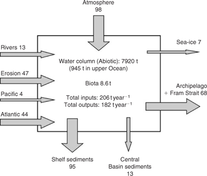
Our analysis of the available data indicates that a total Hg mass of ~7930 t is held in the abiotic and biotic compartments (excluding shelf and basin sediments), of which 99.9% is in abiotic forms (i.e. 7920 t; Fig. 6). In the upper Ocean, ~945 t is abiotic. A surprisingly small amount of Hg resides in marine biota, estimated as <9 t. System inputs total 206 t year–1, with the largest contributions from the atmosphere (98 t year–1 or 48%), oceanic inflows (48 t year–1, 23%) and coastal erosion (47 t year–1, 23%). Wet deposition throughout the year, followed by springtime MDEs, are the important atmospheric processes; our calculations indicate dry deposition (dustfall) is inconsequential. Confidence in the budget is increased because the average Hg turn-over times for the upper Ocean and whole Ocean based on these figures (~5 and 38 years, respectively) approximate water residence times, i.e. ~10 years for the Haloclines and Polar Mixed Layer, and 25–75 years for Arctic Deep Water and the Atlantic Layer.[ 28 ] Mercury outputs of 182 t year–1 are dominated by sequestration in shelf sediments (95 t year–1) and seawater export (68 t year–1). The model therefore portrays a system close to steady-state, with a negligible net gain of 24 t year–1 (~0.3% of total mass). This outcome is consistent with global ocean Hg budgets,[ 52 , 53 , 87 ] which indicate <0.2–0.7% annual increase in the seawater inventory. Virtually all of the global Hg increase accumulates in deep waters below 500 m,[ 52 , 53 ] a finding implying that vertical (downward) flux plays a crucial role in the oceanic distribution of Hg.
|
The relative importance of input and output pathways differs substantially between the Arctic and other oceans (see refs [52,88]). Outputs in global oceans are dominated by GEM evasion (70%), whereas sedimentation results in only small losses. In contrast, evasion in the Arctic is negligible as expected (10 t year–1 or 5%), and sedimentation dominates (56% of outputs). Atmospheric flux accounts for more than 90% of global ocean inputs, but slightly less than 50% in the Arctic, similarly to the Mediterranean Sea,[ 24 ] another semi-enclosed ‘small ocean’. Because the influx from the atmosphere is maximised in the present study (i.e. 98 t year–1), the conclusion that the atmosphere is less dominant in the Arctic than in other oceans is robust, despite continuing uncertainties about the actual amount of Hg re-emission after MDEs and the resultant net input. Therefore, we also deduce that the overall influence of anthropogenic inputs via the atmosphere is proportionately less in the Arctic than elsewhere.
The near-equivalence of the two largest input and output terms for the Arctic Ocean – atmospheric deposition and losses to shelf sediments – suggests that a rapid scavenging and sedimentation of deposited Hg may take place in the euphotic zone during spring and summer. This interpretation is supported by two pieces of evidence. First, it is consistent with the new seawater total Hg profiles presented here (Fig. 5). Most of the sampling stations, except those in Baffin Bay, exhibited a distinct minimum in total Hg at ~50 m compared with surface and 100–200-m waters. Laurier et al.[ 77 ] observed a similar pattern in the North Pacific Subtropical and sub-Arctic gyres and suggested that rapid downward flux of particulate-bound Hg was the explanation. A study of particulate Hg in surface seawater north of Svalbard showed that volume-based concentrations of suspended particulate matter (SPM, mostly of marine algal origin) were inversely correlated with SPM Hg concentrations during summer and fall.[ 76 ] This result could be explained by biomass growth-dilution of Hg adsorption onto SPM, suggesting that dissolved Hg was in limited supply in the euphotic zone by the end of the growing season, although the finding needs to be confirmed by further research.
Lessons about the fulcrums controlling biological Hg trends
One important implication from the current study is that recent increases of biotic Hg in the Arctic Ocean cannot be explained by loadings from the atmosphere or any other import pathway. Seawater and biological Hg concentrations are likely to exhibit only slow, muted responses to increasing or decreasing inputs; owing to the reduced role of the atmospheric pathway, the Arctic’s response to atmospheric loadings will be even more gradual than that of other oceans (see ref. [52]). The mass balance suggests an Arctic Ocean close to steady-state in terms of influxes and effluxes, whereas the biological trend data from Canada and Greenland suggest relatively rapid Hg increases. These findings are not necessarily contradictory, but they cannot be reconciled by a purely mass-driven interpretation and so other explanations must be invoked.
There are multiple lines of evidence and reasoning supporting this interpretation. First, the large mass of Hg already in the system confers a high degree of inertia on seawater and biological responses to the relatively small annual inputs from the atmosphere and other pathways (the ‘flywheel effect’). High mass systems are inherently less responsive to minor inputs than low mass systems. The best estimate of net total Hg increase (0.3% year–1 of the extant inventory) corresponds to a doubling of the oceanic reservoir in ~250 years. If this rate had been sustained over the last century, mass inputs alone could plausibly explain the long-term biotic Hg increases since the pre-industrial period (see also ref. [52]), but not the rapid increases and marked variations of recent decades. This conclusion is unaffected by reasonable alternative choices for seawater Hg concentrations in the inventory calculation (see above), and it supports and extends the suggestion of St. Louis et al.[ 54 ] that meltwater Hg inputs have a limited impact on Arctic seawater concentrations. An alternative interpretation could be that most of the standing oceanic inventory is not bioavailable; with a small and rapidly cycling pool of bioavailable Hg, inputs that are quickly converted to bioavailable forms could produce a rapid biotic response proportional to the input, as they do in lakes (see ref. [89]). However, this interpretation is not supported by MeHg inventory calculations for the Arctic Ocean, which lead to the striking finding that most of the MeHg already in the upper Ocean is not accumulated by marine biota, i.e. it remains in abiotic form. Earlier it was calculated that Arctic marine biota contain 8.6 t total Hg (see Table 6). Assuming that MeHg comprises no more than 25% of total Hg in bacteria, phytoplankton and zooplankton,[ 90 ] and 100% in marine mammals and fish,[ 91 ] the MeHg mass in marine biota is therefore ~4.5 t. We conservatively estimate that 47 t of abiotic MeHg (~5% of the total Hg pool) is present in the upper Ocean, and ~450 t in the whole Ocean, based on a dissolved MeHg concentration of 0.03 ng L–1 measured in North Atlantic continental shelf waters.[ 92 ] Thus, bioaccumulated MeHg represents <10% of the dissolved MeHg pool in the upper Ocean alone, and <1% of whole Ocean MeHg. If the extant pool of bioavailable MeHg is already >10-fold larger than that that has been bioaccumulated, then the effect of further additions to that pool must be limited proportionately.
Indeed, the above calculations suggest that Hg speciation and bioavailability (specifically, dissolved MeHg concentration) may not be a generally limiting factor on Hg concentrations in Arctic marine biota. This is surprising because MeHg is regarded as an extremely bioavailable Hg species whose assimilation by aquatic food-webs is rapid, of the order of days.[ 36 , 89 ] However, another example of an apparent excess abundance of MeHg occurs in Alaskan lakes, in which MeHg accumulation by fish accounted for only 2–14% of annual MeHg inputs.[ 93 ] In contrast, in a temperate coastal food-web, over half of the MeHg inputs were assimilated annually.[ 94 ] Our interpretation of the Arctic Ocean data is unaffected by the selection of dissolved MeHg concentrations as low as 0.005 ng L–1 (at which point abiotic and biotic MeHg pools would be approximately equal). Furthermore, the estimate of the abiotic MeHg reservoir probably understates its true size, because dissolved MeHg concentrations several times higher than those used in the present calculation were determined in surface waters of the Canadian Arctic Archipelago.[ 54 ]
A second argument against recent mass-driven biotic Hg trends is that the calculated total Hg inventory increase of 0.3% per year is at least several times lower than the rate of biological Hg increase. Even the highest plausible net input of ~50 t year–1 (see Table 3) is equivalent to an inventory increase of only ~0.6% per year. Biotic Hg increases are at least several times more rapid. In stating this, it must be assumed that biotic data from the Beaufort Sea and the Canadian Archipelago and west Greenland outflow region represent the Arctic Ocean as a whole, given the absence of data from the Siberian Arctic and the fact that other datasets from the North Atlantic lie outside the budget area. Two of the longest and most robust Arctic datasets concern Beaufort Sea beluga, in which annual increases of liver Hg were ~25% between the early 1980s and mid-1990s,[ 5 ] and two species of Arctic-resident sea-birds (northern fulmars and thick-billed murres) in the Canadian Arctic Archipelago,[ 95 ] which exhibit egg Hg increases of 1.8–2.6% per year since 1975. Other datasets show intermediate rates of increase[ 4 ]; thus, all of the biological rates were well above the maximum mass inventory increase of 0.6%.
The mass-driven interpretation furthermore fails to account for significant differences between co-occurring species, which may exhibit non-linear trends, substantial year-to-year changes, varying rates of change, and even reversals of trends within the same general area.[ 4 ] Most datasets do not display the consistently increasing pattern determined in the sea-bird eggs. The Beaufort beluga trend, as one example, shows that subsequent to a maximum reached in 1996, age-corrected liver Hg levels declined by about half up to 2005.[ 5 , 96 ] In fact, several biotic Hg trends across the Arctic, whether increasing or decreasing, display significant non-linear components,[ 86 , 97 ] which indicate that simple Hg mass increases or decreases in the Arctic are not the principal drivers of biotic Hg variation over recent decades.
The recent impact of mass inputs, especially of atmospheric origin, is also brought into question by the lack of an obvious MDE-related signal in Arctic surface seawater. According to the GRAHM model, MDE-associated deposition delivers within a few weeks in springtime almost half of the atmospheric input and ~20% of total inputs to the Arctic Ocean. Unfiltered (total) Hg profiles from the Beaufort Sea and Archipelago in summer 2005 (see Fig. 5) did not show significantly elevated Hg levels in surface waters as is observed in mid-latitude ocean profiles as a consequence of a dominant atmospheric input.[ 74 , 77 , 88 , 98 ] In Baffin Bay, a single site with higher surface concentrations (1.19 ± 0.19 ng L–1) than elsewhere, skewed the overall mean (see Fig. 5a). If this value is removed, the Baffin Bay surface values average 0.51 ± 0.06 ng L–1, similar to or lower than those deeper in the profile. An alternative explanation for the apparent absence of an MDE effect is that the summer sampling campaign failed to collect the springtime pulse of MDE Hg, which was rapidly absorbed by marine food-webs. However, this seems unlikely in view of the minor fraction of Hg held in biota, which is five times smaller than the model’s springtime input of 45 t. The report of Stern and Macdonald[ 90 ] of increased MeHg levels in Beaufort Sea zooplankton around the time of snowmelt may be evidence of this pulse on a local scale; it may also simply reflect increased local microbial methylation or zooplankton growth rates, driven by warmer water temperatures and snowmelt nutrients. Arctic cod sampled at the same times and locations did not show an increase.
The conclusion that recent Hg trends in Arctic marine biota are not mass-driven is contrary to past experience from freshwater systems concerning the impact of atmospheric inputs on Hg in food-webs. Spatial patterns of MeHg in freshwater biota are correlated with regional variations in atmospheric Hg deposition across Europe and North America,[ 99 – 102 ] and mesocosm isotope spike experiments[ 89 ] and lake mass balance studies[ 20 , 93 ] confirm the importance of atmospheric HgII inputs for MeHg cycling and biotic uptake in lakes. However, the Arctic Ocean and other oceans are fundamentally different from lakes, not least because of their large extant Hg inventories compared with relatively minor loadings (see also ref. [52]), which are a function of smaller surface area : volume ratios. This is further exacerbated by the diminished role of the atmosphere in the Arctic compared with other oceans.
Alternative drivers of changes in biotic Hg
If ‘bottom-up’ controls (i.e. the concentrations of bioavailable Hg in seawater driven by mass inputs and Hg speciation) are incapable of satisfactorily explaining Hg increases and variations in marine biota as we propose, then other processes must be considered. We suggest the alternative explanation that the rate of biological uptake and trophic transfer from the large abiotic MeHg reservoir may be a key regulator. Processes that might be involved in this form of regulation could include: food-web ecology (e.g. changing food-web species composition, foraging domain, or the efficiency of zooplankton grazing of phytoplankton biomass[ 103 ]); ocean biogeochemistry (e.g. variable inputs of key nutrients that limit Hg incorporation by phytoplankton); plant and animal physiology (growth rates and metabolism); and animal ecology (sea-ice-limited access of animals to shelf areas where seawater and food-web MeHg concentrations may be higher (see ref. [90])). The possible role of ocean grazing ‘match–mismatch’ (i.e. the degree of coupling in time and space of phytoplankton blooms and large zooplankton stocks[ 103 ]) is particularly intriguing because it can directly influence the capture efficiency of organic carbon and nutrients (and logically also contaminants) by Arctic marine food-webs. It is also climate-sensitive, as are many of the above processes, and can exhibit significant variations annually as well as geographically,[ 103 ] which could partly account for annual and regional biotic Hg variations. Grazing mismatch could represent a possible ‘break-point’ for Hg flows in food-webs, between effective incorporation into the primary consumer trophic level, and diversion of Hg out of food-webs by sedimentation of ungrazed algal biomass (i.e. pelagic–benthic coupling v. pelagic–pelagic coupling).
It would be premature to conclude, on the basis of the apparent excess abundance of unaccumulated MeHg, that Hg methylation plays no role in determining biotic Hg concentrations. Arctic Ocean Hg speciation, bioavailability and bioaccumulation are processes about which we know very little at present. The presence of unusually high seawater MeHg concentrations under sea-ice just before ice breakup, without corresponding elevations of total Hg,[ 54 ] suggests that over-winter changes in aqueous Hg speciation (mediated through increased methylation or decreased demethylation rates) could be an important fulcrum for biological Hg uptake in springtime, at least in localised areas such as open ice leads and polynyas. Furthermore, processes such as blowing snow entering polynyas might provide locally important pathways between MDEs and biological uptake that are missed by examining only large-scale balances between deposition and emission at the snowpack surface. Nonetheless, our present understanding of Hg inventories and fluxes in the Arctic Ocean strongly suggests that we should look to marine ecology and biogeochemistry for the explanation for recent biotic Hg trends. The governing factors for local production of MeHg, where and at what rate MeHg is captured by ambient biota, and its transfer efficiency through food-webs, are probably centrally important questions to answer on the way to understanding why biotic Hg is increasing in the Arctic Ocean and decreasing in the North Atlantic, and why there is significant variation within these regions, between years, and between species.
Uncertainties and future research priorities
Outcomes and conclusions from the flux calculations are sensitive to uncertainties and inadequacies in the sometimes limited datasets used to formulate them. New findings could easily change the conclusion about a quasi steady-state between inputs and outputs. However, conclusions stemming from comparisons of biotic Hg mass v. the large abiotic Hg reservoir in the Ocean, and in particular the size of the unincorporated MeHg pool, are more robust because the calculations are simpler and based on generally better-quality data, and the masses involved are starkly different from each other. Those values depend on volume data for the Arctic Ocean that are accurately known,[ 104 ] conservatively estimated seawater Hg and MeHg concentrations, and Hg concentrations and biomass of the major groups of marine biota. Although these latter data are less accurately known than seawater volume and Hg concentrations, the conclusions would remain valid even if the true biotic Hg and MeHg inventories had been underestimated by 10-fold.
Based on the relative magnitude of Hg pathways into and out of the marine system, and the differences between the minimum and maximum flux estimates (which reflect either inherent variability or an undersampling of those pathways), future development of the mass balance inventory would benefit most from improving precision and accuracy of the following parameters: the net atmospheric Hg contribution (after re-emission and evasion); waterborne Hg exchange between the Pacific, Atlantic and Arctic Oceans; Hg input from coastal erosion; Hg sequestration into continental shelf sediments; and marine biota Hg mass. Studies on water-column Hg scavenging and vertical flux should form part of this work. Development of a MeHg mass balance would improve our understanding of factors controlling Hg flows into and through food-webs, and so additional MeHg studies on many of the same parameters are required.
Our conclusion that the atmosphere is less dominant in the Arctic Ocean than elsewhere is conservative, for reasons discussed above. Nonetheless, uncertainty around the true magnitude of the net atmospheric flux is particularly problematic because this largest single input in the budget is presently very uncertainly estimated given the order-of-magnitude difference between model results and calculations based on measurements. In part, this uncertainty reflects past misjudgements by the scientific community about the relative significance of MDEs v. other atmospheric processes that occur year-round, and about the actual role of the atmosphere compared with other Hg pathways. In contrast to a sizeable literature and on-going programs in several Arctic countries examining MDE chemistry or monitoring GEM trends, no comparable effort has been directed towards wet deposition. As far as is known, wet deposition monitoring in the Arctic currently takes place at only one site in the Canadian sub-Arctic,[ 71 ] and no related process research or dry deposition monitoring occurs or is planned. Furthermore, irrespective of the uncertainty around the net atmospheric flux, other pathways in total contribute at least as much Hg to the Arctic Ocean. We strongly hold the view that further substantive progress on understanding the risk presented by Hg to Arctic marine biota and their human consumers will stall without a systems approach to research that includes processes in the upper Ocean. Given the new quantitative perspective provided here, a realignment of funding priorities may be in order.
Another part of the reason for uncertainty over the atmospheric input is the lack of consensus about the best approach to measure the net impact of MDEs and re-emission. As mentioned, there is considerable disagreement between the results of snowpack-based and atmospheric gas dynamics approaches. If it is assumed that meltwater runoff is the only important route for MDE Hg in sea-ice snowpacks to enter the ocean, then delivery of 45 t year–1 of atmospheric Hg in spring as estimated by the GRAHM model would require meltwater Hg concentrations to be up to five times higher (~15 ng L–1) on average than the present literature reports (see Fig. 4), and be sustained at those levels across the Arctic Ocean throughout the entire melt period. Delivery of 300 t of Hg annually from MDEs alone, as earlier models proposed, would require ~40-fold higher meltwater concentrations. At present, the literature concerning Hg in snowpack runoff presents a relatively consistent set of findings, but possible methodological flaws should be considered. It is possible that some of the meltwater studies did not sample frequently enough or at the right stage of the melt cycle to capture a large pulse of Hg exiting the snowpack; meltwater Hg concentrations can vary considerably within 24 h.[ 105 , 106 ] However, other studies[ 15 , 105 ] conducted frequent and lengthy sampling campaigns. There is a need for co-located studies using both approaches (to unravel methodological issues from real geographic variability) to be carried out at multiple locations across the Arctic.
Processes and pathways sensitive to climate change
Recent climate warming has had and is projected to have profound effects on virtually all aspects of the Arctic, including biogeochemical cycles.[ 28 , 107 ] Here, we discuss how projected changes in environmental processes and pathways might significantly influence environmental Hg fluxes or biological Hg levels (summarised in Table 8).
|
One of the most pervasive and influential geophysical factors having potential to affect marine Hg dynamics is sea-ice. Together with snow cover, the extent and thickness of sea-ice are involved in a positive feedback loop with the albedo effect on the absorption rate of solar energy by the Arctic Ocean, which has the potential to force many processes across tipping-point thresholds beyond which rates of change become non-linear relative to air temperature trends. Relatively small changes (of the order of a few weeks) in the timing of sea-ice breakup and freeze-up, for example, are likely to have disproportionate effects on the physical forcing of Arctic heat, light and nutrient budgets, and may already be having measurable impacts.[ 28 , 107 ] The Arctic Climate Impact Assessment’s median projection of sea-ice extent in 2070 was a 26% reduction from 2000 levels, with more severe and immediate effects in spring and fall and on ocean margins.[ 107 ] By 2020, sea-ice extent is predicted to be so reduced that continental shelves will be mostly ice-free in summer, with resulting ‘substantial’ increases in nutrient loadings because of wind-driven sediment resuspension and upwelling of nutrient-rich deeper waters.[ 107 ] Recent observations suggest that this rate of ice retreat might be a gross underestimate,[ 108 ] with some predicting an entirely ice-free summer Arctic Ocean before 2020.[ 109 ] The present discussion will concentrate on DGM evasion; MDEs; coastal erosion and permafrost loss; marine primary productivity, scavenging and sedimentation; and Hg methylation–demethylation, because these processes are all exceptionally sensitive to change in the cryosphere and most of them contain the largest budget terms. We assume that the net effect of climate warming on Arctic seawater inflows and outflows will be minimal, although circulation patterns are expected to change.[ 107 ]
Evasion. Summertime evasion could become a major Hg removal process from continental shelves in a warmer Arctic Ocean, as it is presently in the Baltic Sea.[ 56 , 58 ] There is already an active microbial community present in Arctic seawater capable of reducing environmentally significant amounts of inorganic HgII,[ 110 ] and the shrinking area of sea-ice will increase UV radiation penetration and therefore probably photoreduction of HgII to Hg0. The present latitudinal gradient of oceanic GEM evasion can be used to project future increases for the Arctic. Reduction of oceanic HgII in summer increases exponentially between 80–90°N and 60°N because of greater microbial metabolism in temperate ocean upwelling regions; rates in productive coastal areas are also higher than average.[ 53 ] Consequently, summer GEM efflux increases from ~50 to 400 ng m–2 month–1, and annual flux from near-zero to 200 ng m–2 month–1, between those latitudes. The latter rate would be equivalent to an Arctic Ocean-wide efflux of 23 t year–1, although the St. Louis et al.[ 54 ] data suggest that this might be an underestimate. Their calculated GEM efflux of 130 ± 30 ng m–2 day–1 just before ice breakup scales up to 37 t of Hg released in only 1 month.
Mercury depletion events. Springtime MDEs require abundant sea salt aerosols in the lower troposphere, calm weather, a temperature inversion, sunlight and subzero temperatures.[ 63 , 73 ] Predicting the impact of a warmer climate on MDE Hg fluxes is speculative owing to the unknown effects of simultaneous and possibly opposing trends in these parameters. Because MDEs presently cause atmospheric GEM concentrations to commonly decline below 0.1 ng m–3,[ 13 ] the potential to amplify Hg flux per MDE appears to be limited. However, climate factors that increase the frequency, geographic extent or location of MDEs offer more scope. The initial stages of climate change may enhance MDE frequency around Arctic Ocean margins because of more first year sea-ice, which ultimately will contribute larger amounts of BrO and ClO aerosols to the marine boundary layer. Larger areas of new sea-ice and open ice leads than at present should increase MDE intrusion into the Central Basin. By 2050, though, predictions are that average winter sea-ice extent will have declined by 15 to 20% and summer sea-ice by 30 to 50%.[ 107 ] Under these conditions, although new ice may be a larger percentage of total ice cover, the overall new ice area may be smaller than at present. Thus, longer-term warming may reduce opportunities for MDE occurrence around Arctic Ocean margins, but increase its occurrence over the interior ocean. More open water will also result in proportionately more RGM and HgP being deposited directly into seawater, which should reduce the relative amount of re-emission.
Coastal erosion and permafrost loss. Permafrost may play a role in stabilising Arctic soils and marine sediments through mechanical bonding of particles, and is a repository of massive deposits of Holocene terrestrial organic matter,[ 107 ] which probably contain a globally significant but as yet unquantified mass of Hg. Surface soils in the Arctic likely contain some portion of contaminant Hg that has been deposited during the past two centuries; changes in soil moisture and temperature cycles may therefore release this archived Hg or enhance its methylation. Quantitative predictions of future erosion rates in Arctic catchment and coastal areas are lacking. However, large reductions in the depth and extent of terrestrial, subsea and coastal permafrost are probable in a warmer Arctic, and the frequency and severity of storms in the Arctic will also increase.[ 107 ] Both of these trends are likely to significantly elevate erosion of soil from coastal bluffs and riverbanks and of sediment from beach deposits, thus enhancing the fluxes of Hg and ancient organic matter into near-shore areas.[ 28 , 111 ] Given that Arctic riverine particulate organic carbon (POC) tends to be old, and is thought to derive from riverbank erosion, and dissolved organic carbon (DOC) is young and derives from leaching of shallow soils,[ 46 ] we expect that release of archived contaminant Hg will likely follow the DOC (and colloidal organic carbon) pathway. Long-term permafrost borehole temperature records from across Siberia, Scandinavia and the Canadian Arctic have shown increases of 1°C or more in recent decades.[ 112 – 114 ] Modelled estimates of the area of terrestrial permafrost retreat range from 13 to 29% up to 2050, with increases in the depth of seasonal thaw varying regionally from <10 to >50%.[ 107 ] Similar estimates were not forthcoming for coastal and subsea permafrost because of inherent system complexity and unpredictability.
Marine primary productivity and Hg scavenging and sedimentation. Sea-ice cover is presently one of the key factors regulating Arctic Ocean primary productivity and biomass.[ 115 ] In a future with less ice, higher nutrient levels and the improved light climate in seawater will likely drive marine primary productivity (MPP) higher by about two to four times above present in shelf waters such as the Barents Sea, with smaller increases in the upper Central Basin.[ 103 ] Increasing primary productivity has been found to reduce Hg bioaccumulation in higher consumer species in laboratory and natural freshwaters, by reducing per cell Hg accumulation by phytoplankton.[ 116 , 117 ] There is limited evidence that this effect occurs in Arctic marine phytoplankton.[ 76 ] Another possible effect of greater climate-driven aquatic productivity will be to increase the rate of waterborne Hg scavenging and sedimentation by algal-derived particulate organic matter, as was recently demonstrated in High Arctic lakes.[ 22 , 118 ] Although no empirical data are yet available for this phenomenon in marine systems, the overall effect of greater MPP will likely be to lower Hg levels in marine biota, partly by growth dilution at the bottom of food-webs and partly by enhanced vertical flux into the deep ocean.
Methylation–demethylation. The finding that the abiotic MeHg reservoir in the upper Ocean is many times larger than the mass held in marine biota raises doubts about whether and how rapidly future changes in methylation process rates would significantly impact biotic MeHg levels. Ultimately, however, changes in Hg speciation have the potential to leverage dramatic change in biotic Hg levels because of the multiplicative effect of MeHg biomagnification, which can increase Hg concentrations in consumer animals 1000–3000 times above that in particulate organic matter.[ 119 , 120 ]
The findings of high DGM concentrations under sea-ice in spring, and of a high proportion of MeHg in Archipelago sea-water[ 54 ] indicates the presence of an active, cold- and Hg-resistant microbial community capable of significantly affecting aquatic Hg speciation (see ref. [110]). Temperature and organic matter are two key influences on methylation activity in marine and estuarine sediments.[ 36 ] Future sea surface temperatures are likely to increase by approximately the same rate as air temperatures in areas free of sea-ice, but will remain near freezing in areas with long-term ice cover.[ 107 ] If so, Arctic Ocean margins will likely see average water temperatures increase by ~4°C in winter and 0.5–1.0°C in summer by 2050.[ 107 ] In shallow Arctic ponds where summer water temperatures varied by over 15°C, increasing temperatures led to higher dissolved total Hg and a significant increase of up to 40% in the MeHg proportion of total Hg.[ 121 ] Although these temperature ranges are unlikely to be experienced by marine ecosystems, drainage of organic carbon and Hg from melting permafrost into shallow, turbid estuaries and littoral zones, or into shallow coastal lakes that drain to the sea, could increase methylation activity in these areas as they warm, and enhance MeHg inputs to near-shore food-webs.
Demethylation has been poorly investigated compared with methylation, but it is known to occur through both biotic and abiotic processes and to be a particularly important part of the Hg cycle in sediments.[ 36 ] In temperate estuarine sediments, cycling of Hg by biotic methylation–demethylation was rapid with a turn-over time for MeHg of the order of days.[ 92 ] Photodemethylation was a potent process in an Alaskan lake, accounting for ~80% of annual sedimentary MeHg production, even though it was limited to the 100-day ice-free season.[ 122 ] In essence, photodemethylation competed with freshwater biota for MeHg, thereby possibly inhibiting its uptake by the lake’s food-web.[ 122 ] For the Arctic Ocean, future changes in overall demethylation rates and the possible impacts on biotic Hg are difficult to predict. Potential photodegradation increases as a result of longer ice-free seasons may be offset by greater light attenuation by more standing phytoplankton biomass and dissolved organic matter. The effect of increased temperature and organic matter on microbial demethylation has not been investigated, but can be expected to promote those processes. However, in a study of demethylation across freshwater environments that differed in Hg contamination and sediment characteristics, total Hg concentration was found to be the most important determinant of microbial demethylation rate, exhibiting a significant positive relationship.[ 123 ] Biogeochemical factors, however, were of negligible influence, suggesting that overall changes in demethylation rates may be minimal in a warmer Arctic. The net result of future changes in methylation and demethylation may therefore be increased Hg methylation potential.
Conclusions
Development of the present Hg mass balance has produced some unexpected findings concerning the state of Hg fluxes and masses in various Arctic Ocean compartments, and their potential impact on biotic Hg temporal trends and variations. Like global oceans in general, Hg influxes and effluxes in the Arctic Ocean are close to steady-state, with a small net annual increase equivalent to a doubling of oceanic Hg concentrations in ~250 years. Atmospheric inputs are less dominant for the Arctic than for other oceans (<50% of total inputs v. 90%, respectively), and so the importance of anthropogenic loadings via this pathway is proportionately diminished. Evidence that MDEs in spring significantly influence Arctic seawater or marine biota Hg concentrations continues to be elusive. Even with the atmospheric input maximised in this inventory, MDEs contributed <22% of total inputs (all pathways) and <50% of net atmospheric inputs. Arctic seawater Hg profiles published here for the first time also show no evidence of surface enrichments consistent with a dominant atmospheric or springtime MDE impact. Rapid scavenging and downward export of dissolved Hg from seawater by algal-derived particulate organic matter may operate as a steady-state counterweight to airborne Hg deposition in the surface ocean.
The currently large abiotic total Hg and MeHg inventories in Arctic seawater confer a high degree of inertia on change in seawater and biotic Hg concentrations. We infer that ‘bottom-up’ processes (i.e. control of bioavailable Hg concentrations in seawater by mass inputs and Hg speciation) are not capable of directly regulating biological Hg levels and trends, at least not generally. We propose instead that ‘top-down’ processes, i.e. the rate of biouptake and trophic transfer by marine food-webs from the dissolved MeHg pool, are likely to be key variables and that these in turn depend on other processes possibly including food-web ecology, animal foraging strategy, physiology, nutrient biogeochemistry, and sea-ice control of animal access to continental shelf areas. These should prove to be fruitful areas for future research, especially as all are potentially climate-sensitive.
A policy-related implication from this mass balance is that while pollution-driven increases of net inputs, sustained over the long term, could produce the dramatic Hg increases that have occurred in Arctic marine wildlife since pre-industrial times, trends in recent emissions are not capable of producing the rapid increases occurring over recent decades. Future reductions in global atmospheric Hg emissions, although necessary to return Arctic biotic Hg levels to their natural state, will probably produce only gradual, long-term reductions in seawater and biological Hg concentrations, unlike in lakes. The response of the Arctic Ocean, because of the weaker atmospheric influence, will be even slower than the muted response to emission controls predicted for other oceans.
Although uncertainty about flux and mass estimates is to be expected when developing a first-order model based on limited data, the conclusions stated above are robust across a wide range of alternative selections of concentrations and water and sediment mass transfers. The best-estimate concentrations and pathway transfer coefficients were conservatively chosen, and the range of minimum to maximum estimates of net flux (+11 to +47 t year–1) indicate that overall uncertainty around the best estimate of +24 t year–1 is probably about ±100%. Also, the contrast between the biotic and abiotic masses of total and MeHg is so striking that even an order of magnitude error in estimation would not seriously challenge the resulting conclusions. Thus, although the precision and accuracy of inventory numbers will benefit from future research and can be adjusted accordingly, there are grounds for a high degree of confidence in the general findings and conclusions.
The effects of climate warming in the Arctic, particularly retreat of sea-ice, are likely to bring about profound changes of Hg fluxes in the Arctic Ocean. Although quantitative prediction is not presently possible, the change in sea-ice regime will likely force large amounts of Hg out of the euphotic zone through higher evasion and greater downward fluxes driven by increased primary productivity and scavenging. Opposing the resulting ocean-wide decreases, we expect elevated inputs from coastal erosion into ocean margins, and smaller increases from flushing of archived natural and contaminant Hg in river catchments. These latter processes might be locally significant. In terms of Hg bioaccumulation, higher marine algal productivity could enhance biomass dilution of Hg at the bottom of food-webs and thus reduce Hg uptake by higher consumer animals. The overall impact of a warmer Arctic Ocean on these pathways and processes is likely to be reduced seawater levels followed by slower declines in biotic Hg concentrations.
Experimental methods for seawater Hg profiles
Seawater samples from the Beaufort Sea and Canadian Arctic Archipelago were collected on board the Canadian Research Icebreaker CCGS Amundsen in July–August 2005 as part of an ArcticNET research cruise. The samples were collected from various depths of the water column in pre-cleaned Niskin bottles (General Oceanics, Miami, FL). The samples were stored in 50-mL new sterilised Falcon polypropylene tubes (VWR, Missisauga, ON) that were tested for background Hg levels (always <0.1 ng L–1) before being shipped to the field. Once filled with samples in the field, the bottles were double-bagged in polyethylene Ziploc bags and transported in coolers to the laboratory where they were refrigerated until analysis. The two-person ‘clean hands, dirty hands’ Hg sampling protocol[ 124 ] was followed to minimise potential contamination.
The analysis of total Hg in seawater samples was performed as described previously[ 83 ] by cold-vapour atomic fluorescence spectroscopy on a Tekran 2600 Hg analyser (Tekran Instruments Corporation, Knoxville, TS) in Class 10–1000 clean-rooms at the metal-free, Ultra-Clean Trace Elements Laboratory (UCTEL) of the University of Manitoba, following US EPA Method 1631.[ 125 ] Certified reference material ORMS-3 (National Research Council of Canada) was used for quality control, and results were within 5% of their certified values. Further quality assurance and quality control were carried out regularly in the laboratory as part of the interlaboratory comparison program under the Collaborative Mercury Research Network (COMERN) and the Metals in the Human Environment Research Network (MITHE-RN).

|
Acknowledgements
The new Arctic seawater Hg results incorporated here were made possible by multi-year funding from the ArcticNET Network of Centres of Excellence to R.M., G.S. and F.W. We also acknowledge past support from the Geological Survey of Canada (P.O.), the Science Subvention Program of the Department of Fisheries and Oceans and the Fisheries Joint Management Committee (F.W., G.S.), the Polar Continental Shelf Project (F.W., G.S.), the Canadian Arctic Shelf Exchange Study (CASES; G.S., R.M.), and the Natural Science and Engineering Research Council of Canada (F.W.). P.O. thanks Prof. Bill Shotyk and the Institute for Environmental Geochemistry, University of Heidelberg, Germany, for hosting him during the preparation of the present article. We also thank Dr Alison Green for the invitation to prepare the present review for Environmental Chemistry, and to the Arctic Monitoring and Assessment Program (AMAP) for permission to adapt Fig. 2 (taken from [ 25 ]). Two anonymous reviewers provided numerous suggestions that have helped to improve the presentation.
[1]
[2]
[3]
[4]
B. M. Braune ,
P. M. Outridge ,
A. T. Fisk ,
D. C. G. Muir ,
P. A. Helm ,
K. Hobbs ,
P. F. Hoekstra ,
M. Kwan ,
R. J. Letcher ,
W. L. Lockhart ,
R. J. Norstrom ,
G. A. Stern ,
Z. Z. Kuryk ,
Persistent organic pollutants and mercury in marine biota of the Canadian Arctic: an overview of spatial and temporal trends.
Sci. Total Environ. 2005
, 351–352, 4.
| Crossref | GoogleScholarGoogle Scholar |
[Verified 17 March 2008].
[87]
C. H. Lamborg ,
W. F. Fitzgerald ,
J. O’Donnell ,
T. Torgerson ,
A non-steady-state compartmental model of global-scale mercury biogeochemistry with interhemispheric gradients.
Geochim. Cosmochim. Acta 2002
, 66, 1105.
| Crossref | GoogleScholarGoogle Scholar |
[Verified 16 March 2008].
[97]
[98]
G. A. Gill ,
W. F. Fitzgerald ,
Vertical mercury distributions in the oceans.
Geochim. Cosmochim. Acta 1988
, 52, 1719.
| Crossref | GoogleScholarGoogle Scholar |
[Verified 17 March 2008].
[126]
A. Ohmura ,
N. Reeh ,
New precipitation and accumulation maps for Greenland.
J. Glaciol. 1991
, 37, 125.
[Verified 17 March 2008].
[140]
C. J. Ashjian ,
R. G. Campbell ,
H. E. Welch ,
M. Butler ,
D. Van Keuren ,
Annual cycle in abundance, distribution, and size in relation to hydrography of important copepod species in the western Arctic Ocean.
Deep-Sea Res. II 2003
, 50, 1235.
| Crossref | GoogleScholarGoogle Scholar |

[141]
K. N. Kosobokova ,
H. Hanssen ,
H.-J. Hirche ,
K. Knickmeier ,
Composition and distribution of zooklankton in the Laptev Sea and adjacent Nansen Basin during summer, 1993.
Polar Biol. 1997
, 19, 63.
| Crossref | GoogleScholarGoogle Scholar |
[142]
M. E. Vinogradov ,
E. A. Shushkina ,
L. P. Lebedeva ,
V. I. Gagarin ,
Mesoplankton in the eastern part of the Kara Sea and Ob and Yenisei Rivers estuaries.
Oceanology (English Translation) 1995
, 34, 716.
[143]
P. Dalpadado ,
R. Ingvldsen ,
A. Hassel ,
Zooplankton biomass variation in relation to climate conditions in the Barents Sea.
Polar Biol. 2003
, 26, 233.
[144]
H.-J. Hirche ,
W. Hagen ,
N. Mumm ,
C. Richter ,
The north-east water polynya, the Greenland Sea III.
Polar Biol. 1994
, 14, 491.
| Crossref | GoogleScholarGoogle Scholar |