

Modelling the impact of possible snowpack emissions of O(3P) and NO2 on photochemistry in the South Pole boundary layer
P. D. Hamer A B D , D. E. Shallcross A , A. Yabushita C and M. Kawasaki CA School of Chemistry, University of Bristol, Cantock’s Close, Bristol, BS8 1TS, United Kingdom.
B Present address: Jet Propulsion Laboratory – NASA, 4800 Oak Grove Drive, MS 183-601, Pasadena, CA 91109, USA.
C Department of Molecular Engineering, Kyoto University, Kyoto, 615-8510, Japan.
D Corresponding author. Email: paul.d.hamer@jpl.nasa.gov
Environmental Chemistry 5(4) 268-273 https://doi.org/10.1071/EN08022
Submitted: 6 March 2008 Accepted: 27 June 2008 Published: 19 August 2008
Environmental context. The study of surface photochemical ozone production on the Antarctic continent has direct relevance to climate change and general air quality and is scientifically noteworthy given the otherwise pristine nature of this environmental region. The identification of possible direct ozone emissions from snow surfaces and their contribution to the already active photochemical pollution present there represents a unique physical phenomenon. This process could have wider global significance for other snow-covered regions and therefore for global climate change.
Abstract. O(3P) emissions due to photolysis of nitrate were recently identified from ice surfaces doped with nitric acid. O(3P) atoms react directly with molecular oxygen to yield ozone. Therefore, these results may have direct bearing on photochemical activity monitored at the South Pole, a site already noted for elevated summertime surface ozone concentrations. NO2 is also produced via the photolysis of nitrate and the firn air contains elevated levels of NO2, which will lead to direct emission of NO2. A photochemical box model was used to probe what effect O(3P) and NO2 emissions have on ozone concentrations within the South Pole boundary layer. The results suggest that these emissions could account for a portion of the observed ozone production at the South Pole and may explain the observed upward fluxes of ozone identified there.
Additional keywords: nitrate and ice chemistry, oxygen atoms, ozone, reaction dynamics.
Introduction
A series of measurement campaigns have highlighted the presence of intense photochemical activity at the South Pole. NOx emissions from the ice due to the photolysis of nitrate cause NO concentrations to reach up to 600 parts per trillion by volume (pptv).[1] Two campaigns have shown that the photochemistry at the South Pole is being driven by the emission of NOx from the snowpack and the changing boundary layer height, which in turn serves to determine the concentration of NOx by affecting the mixing volume.[2] These elevated NOx concentrations lead to in situ production of ozone.[3] NOx is produced within the snowpack from the photolysis of nitrate.[4–6] The exposure that the plateau has during the summer months to 24 h sunlight in conjunction with the photon flux enhancement due to the high surface albedo is important too for determining the photochemical activity.[7,8] Further factors contribute also; the emission of formaldehyde (HCHO) and hydroperoxide (H2O2) from the snowpack[9] has been shown through modelling studies to enhance the HOx budget,[10] while the identification of oxygenated volatile organic compounds (OVOCs)[11,12] and subsequent modelling studies showed that these compounds both impact on ozone production and OH sequestration.[13] Recently published work[13] shows that up to 3–4 parts per billion by volume (ppbv) of the observed ozone results from OVOC oxidation by OH (ozone reaches up to 35 ppbv for sensible OVOC concentrations), but the peak simulated ozone concentrations still fall short of the highest ozone concentrations that are observed at the South Pole (up to 45 ppbv).[3] This discrepancy suggests that there are still some processes missing from within the model. This speculation has perhaps been confirmed by a recent laboratory-based study by Yabushita et al.[14] During their studies, emissions of O(3P) were identified coming from ice films cooled to 100 K that were doped with nitric acid and then exposed to UV–visible light. This is a remarkable discovery and the implications seem to be qualitatively clear from an understanding of reaction 1; the emission of O(3P) should lead to increased ozone production because O(3P) reacts with molecular oxygen via reaction 3 to produce ozone directly. The present study aims to investigate the impact of these emissions using a photochemical box model.


Although the work of Yabushita et al.[14] identified the emission of O(3P) atoms from the ice surface doped with nitric acid, no quantitative estimate was placed either on the quantum yield or on the magnitude of the flux from the ice surface. This is principally because the Resonance Enhanced Multi-Photon Ionization (REMPI) laser technique employed by Yabushita et al.[14] is not a quantitative technique capable of determining the concentration of the species being studied. Further work has been carried out at the South Pole observing both NOx and ozone, investigating the vertical extent of the boundary layer active photochemistry.[15–18] These studies combine in-situ and vertical profile observations of trace gases with meteorological information regarding boundary layer height, wind speed, vertical temperature profile and dew point to further confirm the fundamental role dynamics play in controlling the volume of the boundary layer photochemical reactor, as identified by Davis et al.[2] Helmig et al.[17] observed vertical distributions of NOx from the South Pole for the first time and showed that elevated NOx concentrations only exist within the boundary layer. Johnson et al.[16] and Helmig et al.[18] further confirmed that elevated concentrations of ozone are limited to the boundary layer and become higher during shallow boundary layer conditions. These two studies noted too that under certain conditions, notably when boundary layer heights are lower than 30 m, upward fluxes of ozone appear to exist above the snowpack. A review[19] of ozone dry deposition over snow-covered regions identifies a wide variety of possible ozone deposition velocities, with most studies observing downward fluxes of ozone but with some showing upward fluxes of ozone,[20–23] and as in Johnson et al.[16] and Helmig et al.[18] Ozone is typically dry-deposited over land surface types and many of the vertical ozone profiles from other snow-covered sites exhibit the standard behaviour, i.e. downward fluxes of ozone.[23–27] Indeed, the only regions in the world where upward ozone fluxes have been observed at the surface are snow-covered areas. One intriguing aspect of the recent measurements made at the South Pole[18] was that ozone levels within the snowpack itself were depressed relative to the observations made above the surface. The identification of an upward ozone flux in combination with these results suggests that there is either some unknown process that is inhibiting ozone dry deposition at this location, or it suggests that some process is perhaps producing ozone on the surface of the snowpack or in the first few metres of overlying atmosphere. The present study aims to explore some of these issues.
The present work is aimed at being a follow-up to both the modelling work of Hamer et al.[13] and the laboratory and initial modelling work of Yabushita et al.[14] The aim is to investigate the possible impact that O(3P) and NO2 emissions might have on ozone concentrations in the overlying atmosphere at the South Pole and to compare these results with observations of NO and ozone.
Methods
A photochemical box model was used during the present study. The model was an ASAD-based model[28] (a self-contained atmospheric chemistry code) that was originally constructed to describe urban pollution events. The model consists of two vertically stacked boxes of air, exchange between the boxes, deposition onto the surface in the lower box and transport in and out of the upper box. The model calculates the concentrations of 163 chemical species and includes 472 reactions describing the degradation pathways of non-methane hydrocarbons (NMHCs) containing up to five carbon atoms. This photochemical mechanism is based on the Master Chemical Mechanism.[29] As such, the model has had to undergo a series of modifications in order for it to describe the South Pole boundary layer. The concentrations of NMHCs and other background species had to be reduced from urban levels to the concentrations found at the South Pole. Data from the ISCAT 2000 (Investigation of Sulfur Chemistry in Antarctic Troposphere) campaign provided the basis for this (G. Huey, pers. comm., 2005). The model’s albedo had to be increased from its urban value of 0.3 up to 0.8.[7] NOx emissions had to be speciated so as to emit two NO2 molecules for each NO molecule emitted. This reflects studies of snowpack concentrations of NOx observed during field campaigns at the South Pole and Neumayer.[1,3] Fluxes of both HCHO and H2O2 were added to the model to simulate the observed fluxes of both of these compounds at the South Pole.[9] Following the identification of methyl hydroperoxide (MHP) at the South Pole[12] and the reported presence of other OVOCs there as well,[13] fluxes of OVOCs were added into the box model. Hamer et al.[13] report the sensitivity of the model to various different OVOC scenarios. The OVOC scenario used in the present instance (referred to in the current paper as the ‘Base Case’) was the ‘3 × OVOC’ case. The ‘Base Case’ was then in turn built on using several different O(3P) emission scenarios.
O(3P) was emitted into the lower box (simulating surface emissions) using three different emission factors. Given that the secondary NO3– photolysis leads to the formation of one molecule of NO and one O atom, the emission factors of O(3P) were derived from the ratio between emitted O atoms and emitted NO molecules. The three emission factors used in the model were 0.5, 1 and 2, i.e. one-half of the NO emission, the exact NO emission and twice the NO emission respectively. Each of these O(3P) scenarios was then tested under a range of different boundary layer heights. In each individual model run, the NO and O(3P) emissions were kept constant (2.4 × 10¹⁰ molecules cm–2 s–1) whereas the boundary layer height was changed, thus allowing the full range of NOx conditions to be explored. The surface emissions were larger than the observed emissions by a factor of 100. It is believed that this discrepancy results from the coarse manner in which dynamics are modelled. The venting rates in the model are likely to be too high, which means that higher emissions are required to maintain observed atmospheric concentrations. The following boundary layer heights were used (m): 500, 400, 350, 300, 250, 200, 150, 125, 100, 75, 60, 50, 40, 35 and 30. Further details of the model’s configuration are contained within previous work[13] within the description of ‘run B’.
To solely investigate the contribution of surface NO2 emissions to direct ozone production, two further model investigations were carried out. Using the same model framework of the ‘Base Case’ model being driven by changes in boundary layer height, the NO2 : NO emission ratio was changed. In ‘Control Run 1’, model NO2 emissions were turned off and the model only emitted NO. In ‘Control Run 2’, the NO2 : NO ratio was reversed so that NOx was emitted in a 1 : 2 ratio.
Results
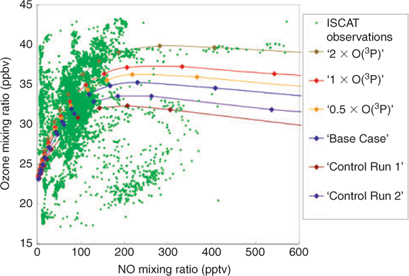
The model results shown in Fig. 1 show how the ozone concentrations from the four different O(3P) emission scenarios vary with changing NO concentration. The NO concentrations in the model were varied by modulating the boundary layer height. The results from the ‘1 × O(3P)’ scenario are viewed as being the most likely representation of reality, given that NO is emitted in a 1 : 1 ratio with O(3P). Comparing the ‘Base Case’ ozone concentrations with the results from the ‘1 × O(3P)’ scenario indicates a difference in ozone concentration of up to ~2 ppbv, whereas the ‘0.5 × O(3P)’ scenario shows a ~1 ppbv increase and the ‘2 × O(3P)’ scenario shows an increase of up to ~5 ppbv.
|
‘Control Run 2’ is lower than the ‘Base Case’ model run by up to ~1.5 ppbv and ‘Control Run 1’ by up to ~3 ppbv, which is the total contribution to ozone production from NO2 emissions. The differences between the ‘Control Runs’ and the ‘Base Case’ results show the contributions to ozone production from direct surface NO2 emissions.
The observations from the ISCAT 2000 monitoring campaign (kindly provided by G. Huey) are shown alongside the model data as green points. These data demonstrate the relationship between ozone and NO concentrations at the South Pole and present a general description of this photochemical environment. It should be noted that ozone concentrations are reaching very elevated concentrations for a clean air location, even with the observed NO levels. Without the presence of the high concentrations of HOx, which also play a key role[10,30,31] at the South Pole, these elevated ozone episodes would not occur. Ozone increases with rising NO concentration in a broadly linear fashion except for two outlying groups of data points. First, there appears to be a series of data points that exhibit very high ozone concentrations while maintaining very low NO concentrations. Second, there appears to be a series of results showing relatively low ozone concentrations that have high NO. In the first instance, these events appear to occur during the break-up of shallow boundary layer conditions and active photochemical episodes exhibiting high ozone and NOx. As the boundary layer height increases, both NOx and ozone begin to decrease, but given that ozone likely has a longer photochemical lifetime under these conditions, it persists longer within the boundary layer. Such an event is visible in the data collected by Helmig et al. in fig. 2,[17] as a sharp increase in boundary layer height occurs and decreases in both NO and ozone are observed, but the key point is that ozone appears to be maintained at higher concentrations for a longer period compared with NO. There are two possibilities in the second instance, though the first seems more likely. Either these data points represent pollution events or something specific about the conditions at the South Pole on that day prevented significant photochemical activity. In the latter case, if it was misty, this could have an impact because mist events were suggested as scavengers for HO2 at the South Pole[31] and HO2 is an important precursor to ozone formation.
Discussion
The significance of the model sensitivities to the differing O(3P) emission scenarios is two-fold. First, the apparent increase in modelled ozone concentration between the ‘Base Case’ scenario and the ‘1 × O(3P)’ scenario indicates that snowpack O(3P) emissions could be contributing to the observed ozone concentrations within the South Pole boundary layer by as much as 2 ppbv, or ~6% of the observed concentration. This figure is in qualitative agreement with the ozone production rate derived from a simple calculation based on boundary layer height and the observed NO fluxes from the South Pole.[32] Assuming a boundary layer height of 20 m and using the observed fluxes from Oncley et al.[32] of 2.6 × 10⁸ molecules cm–2 s–1, a flux (plus assuming that NO and O(3P) emissions are equivalent) into the boundary layer of 1.3 × 10⁵ molecules cm–3 s–1 can be derived, which equates to 0.6 ppbv per day of ozone production. Considering the peak ozone production rate reported by Crawford et al.[3] was 6 ppbv, and the estimated O(3P) production rate is 10% of the observed ozone production rate, there appears to be a decent agreement between the modelled impact of such an emission and its theoretical impact based on field observations. Thus, the predicted absolute concentrations highlight a modest but hitherto unreported source of ozone at the South Pole that is likely contributing to the already active photochemistry present there.
The second implication of the laboratory findings of Yabushita et al.[14] and of the model results presented in the current study is that they have the potential to at least partially explain the apparent upward fluxes of ozone identified at the surface at the South Pole.[16,18] There is another consideration that could place limitations on the applicability of these results to accurately predict the true impact of O(3P) surface fluxes, and, specifically, their potential for explaining the apparent upward ozone fluxes from the snow at the South Pole. This consideration is that the reported ozone concentrations from within firn air at the South Pole are lower compared with the concentrations in the overlying atmosphere.[18] This observation implies that ozone is in fact being destroyed within the snowpack relative to the overlying atmosphere, which is potentially in conflict with the implications presented by the present work. It is assumed here that ozone is being destroyed more efficiently within the snowpack relative to the overlying atmosphere owing to deposition and to a lesser extent by reaction with elevated NOx concentrations[1,3] (see reactions 4 and 5). Although ozone deposition to snow surfaces is believed to be less efficient than to other land surfaces by approximately a factor of 10 (M. King, pers. comm., 2004) the snowpack itself presents a medium with extremely high surface area. Therefore ozone in the firn air will be exposed to a greater deposition loss rate than the overlying atmosphere that only comes into contact with the snow surface. Ozone lifetimes with respect to NOx (3 h in the case of NO and over 100 days for NO2) are considerably longer than the snowpack air residence time (~1 min, derived from Oncley et al.[32]). This suggests that 0.5% of the ozone in the snowpack will be lost via reaction with NO before being vented out of the snowpack.


There are, however, some further points and considerations that could maintain the consistency between the proposed implications in the current work and the firn air ozone observations. First, ozone formed from O(3P) atoms that are emitted directly into the boundary layer from the uppermost snowpack are unlikely to be affected by the three snowpack ozone loss processes mentioned earlier, and so some direct emission of O(3P) into the atmosphere is still possible. Second, the product of reaction 4, NO2, is photochemically active and yields O(3P) atoms on photolysis. NO2 is photolysed via reaction 6 to yield a single O(3P) atom. NO2 formed in this way could act as a potential carrier of O atoms out of the firn air and into the boundary layer.

NO2 has a photochemical lifetime on the order of 6 h (derived via France et al.[33]) in the snowpack and so 99.75% is likely to be transported into the boundary layer before photolysis occurs. This demonstrates that NO2, formed via reaction 4, can act as an effective carrier of O atoms between the firn air and the atmosphere. Assuming a photolysis rate of NO2 in the boundary layer of 1.05 × 10⁻² s–1,[7] NO2 should have a photochemical lifetime of ~1.5 min, and assuming that complete boundary layer mixing is occurring considerably slower than this, it seems highly probable that NO2 formed from reaction 4 that is emitted from the snowpack could contribute to the observed enhancement in surface ozone concentrations. It therefore seems likely that the only process that will inhibit the firn air formation of ozone is the direct deposition of ozone within the snowpack. The depositional loss of ozone within the snowpack may be offset by evaporation of adsorbed ozone and potential for photolysis of adsorbed ozone to re-release O atoms. The work of Yabushita et al.[14] clearly shows that O atoms can be emitted from solid surfaces; it is therefore conceivable that this process could be occurring.
It should also be highlighted that firn air contains elevated concentrations of NO2 with respect to NO in a roughly 2 : 1 ratio[2,4] due to the photodegradation of NO3–, which preferentially photolyses via channel (2) to directly yield NO2. Comparison of the ‘Control Runs’ and the ‘Base Case’ shows the modelled impact on ozone of such emissions. It appears that the direct emission of NO2 from the snowpack increases ozone by as much as 3 ppbv in the model (8.5% of the total concentration at 35 ppbv). This suggests that this is an additional ozone source, even larger than that proposed owing to O(3P) emissions, and that these emissions perhaps go further towards explaining the upward fluxes of ozone observed at the South Pole.
It therefore seems plausible that the following three processes (in order of their magnitude) are contributing to the enhanced ozone production in the air immediately above the snowpack: the emission of NO2 (formed via reaction 2) from the snowpack and its subsequent photolysis (8.5%), direct surface emission of O(3P) from the uppermost snow and to a lesser extent from within the snowpack itself (6%), and the indirect contribution to NO2 production from reaction 4 (~0.01%, see below), i.e. between NO and ozone formed from O(3P) emitted within the snowpack and ozone transported into the snowpack from the overlying atmosphere. The bulk of the latter source is likely to be a result of background ozone reacting with firn air NOx via reaction 4 rather than from ozone formed within the snowpack as a result of O(3P) emission. Assuming that 0.5% of the ozone (assuming a background of 35 ppbv) reacts with NO in the snowpack and that only 6% of this resulted from O(3P) emission, boundary layer enhancements in ozone concentration are likely to be limited to hundredths of ppbv. It is believed that until discrepancies between firn air and boundary layer ozone concentrations can be resolved, the estimate of 6% from O(3P) emissions will be an upper limit for the amount of ozone expected to be produced via this mechanism.
One further explanation for the apparent upward fluxes of ozone is that photochemistry leading to ozone production could be more active in the lower portion of the boundary layer. This could occur simply because NOx concentrations will be elevated closer to the snow surface compared with the upper boundary layer by virtue of proximity to the NOx snowpack source. Indeed, fig. 5 of Helmig et al.[17] shows that a gradient exists in NO concentrations even within a 20–30-m boundary layer, with NO concentrations ranging between 600 pptv at the surface and up to 300 pptv at the top of the boundary layer. Given that the presence of an upward ozone flux was established by examining the difference in concentrations between measurements made at 4 and 17 m, it is entirely possible the gradient in NOx concentrations could be causing the apparent upward ozone gradient. This issue can be investigated using both the model output in Fig. 1 and the observations that indicate a typical NO–ozone relationship. The key point is that ozone production does not seem to change significantly in the range between 200 and 600 pptv of NO according to the model output from the present study and the ISCAT 2000 observations. It is therefore difficult to attribute the observed upward fluxes of ozone to more active low level photochemistry arising from different NOx regimes present at the contrasting altitudes. Therefore, it seems that the explanations postulated previously are more probable.
Further investigation is required to test for the existence of various chemical and physical processes; ozone deposition needs to be thoroughly investigated to determine whether ozone can be photolysed on the ice surface to yield O atoms into the firn air and to see if ozone can be evaporated from the ice surface once it has been adsorbed via a physical process. The budget of NO2 production within firn air needs to be assessed via in-depth modelling and laboratory work to weigh up the relative contributions to NO2 formation via the photochemical processes mentioned earlier.
Another important question is whether or not the central assumptions in the present study are valid. Can the central model scenario of a 1 : 1 emission ratio between O(3P) and NO be justified? Based on the previous discussion, it would appear that this assumption cannot stand without some modification, but more fundamentally, is the emission of radicals from the surfaces of ice particles and from within bulk ice supportable by any observation? In fact, the time-of-flight spectra shown in Yabushita et al.[14] (fig. 3 in that study) shed some light on the microphysics at work on the ice surface and this question. The time-of-flight spectra showed three distinct peaks that from the Boltzmann translational energy distribution can be attributed to different chemical and physical phenomena; the first can be attributed directly to NO3– photolysed on ice surfaces, the second has an energy that corresponds to the lower-energy O atom released from NO2 photolysis also presumably adsorbed onto the ice surface, and the final peak has a translational energy of 100 K relating to O atoms produced within the bulk ice (cooled to 100 K) that have migrated to the surface. The weighting of each O atom source is ~5 : 1 : 4 respectively.[14] The fact that 40% of the observed O atoms are derived from the bulk ice in this experiment is highly supportive of the notion that O atoms produced within ice grains, or near their surface, have a good chance of escaping into the firn air. This adds greater plausibility to the assumption that the 1 : 1 scenario is the most likely reflection of reality. Further, if NO2 adsorbed onto ice grains is also considered as an O atom source, then it appears that a scenario of 1 : 1.1 is perhaps even more probable.
Fig. 1 also shows a comparison between the observations made during the ISCAT 2000 campaign of NO and ozone and the model results. The model appears to broadly agree with the observations, though there are a few areas where the agreement could be better. It should be noted that the model fails to describe the highest ozone concentrations, though the introduction of O(3P) emissions does appear to remove some of this discrepancy. The model also appears to overestimate ozone concentrations at the lowest levels of NO (<50 pptv NO) and underestimate the ozone concentrations at the highest NO levels (i.e. >200 pptv NO). This can be partially attributed to the coarse manner in which the model describes dynamics and the way in which vertical mixing changes as inversions strengthen and the boundary layer shrinks. A fixed rate of vertical mixing is used to vent the upper box of the model and a fixed rate of infilling of free tropospheric ozone is used. In reality, mixing is liable to be more efficient during low NOx conditions, i.e. high boundary layer episodes, and therefore free tropospheric air with lower background ozone concentrations will mix downwards and will tend to lower the ozone concentrations at the surface. Conversely, during high NOx episodes in shallow boundary layer conditions, the model underestimates ozone concentrations and this could be due to overestimation of the rate of mixing between the ozone-poor air of the free troposphere and the ozone-rich air in the boundary layer. Further development work is required to improve the model’s description of these two separate circumstances.
Conclusions
The emissions of O(3P) from nitric acid-doped ice surfaces exposed to UV–visible light is a novel discovery[14] that may have led to a partial explanation of the observed upward fluxes of ozone seen at the South Pole and other locations. However, existing observations of snowpack NO2 suggest that NO2 formed from NO3– photolysis may make a greater contribution to the production of ozone in the lowest portion of the atmosphere above the snowpack. It was also shown that ozone produced in the firn air via O(3P) release and ozone transported into the snowpack can play a minor role in the direct production of NO2.
The increases in absolute modelled ozone concentrations as a result of both simulated O(3P) and NO2 emissions highlight that these processes could have a modest contribution to ozone production at the South Pole. The results clearly show that most of the ozone production can be clearly attributed to the previously reported active photochemistry present there. These newly identified ozone sources are still of note owing to their novel nature.
Acknowledgements
P. D. Hamer would like to thank National Environment Research Council (NERC) and BAS for funding, and Will Harris, Betty Hamer and Laura Watson for special assistance. Special thanks to Greg Huey for allowing access to the ISCAT 2000 dataset and to Doug Davis for extremely helpful discussion. D. E. Shallcross and M. Kawasaki thank the Daiwa Anglo-Japanese Foundation for a Daiwa-Adrian award that supported the current work. A. Yabushita and M. Kawasaki thank the Ministry of Education of Japan for financial support.
[1]
D. D. Davis ,
J. B. Nowak ,
G. Chen ,
M. Buhr ,
R. Arimoto ,
A. Hogan ,
F. Eisele ,
L. Mauldin ,
D. Tanner ,
R. Shetter ,
B. Lefer ,
P. McMurry ,
Unexpected high levels of NO observed at South Pole.
Geophys. Res. Lett. 2001
, 28, 3625.
| Crossref | GoogleScholarGoogle Scholar |

[2]
D. Davis ,
G. Chen ,
M. Buhr ,
J. Crawford ,
D. Lenschow ,
B. Lefer ,
R. Shetter ,
F. Eisele ,
L. Maudlin ,
A. Hogan ,
South Pole NOx chemistry: an assessment of factors controlling variability and absolute levels.
Atmos. Environ. 2004
, 38, 5375.
| Crossref | GoogleScholarGoogle Scholar |
[3]
J. H. Crawford ,
D. D. Davis ,
G. Chen ,
M. Buhr ,
S. Oltmans ,
R. Weller ,
L. Maudlin ,
F. Eisele ,
R. Shetter ,
B. Lefer ,
R. Arimoto ,
A. Hogan ,
Evidence for the photochemical production of ozone at the South Pole surface.
Geophys. Res. Lett. 2001
, 28, 3641.
| Crossref | GoogleScholarGoogle Scholar |
[4]
A. E. Jones ,
R. Weller ,
E. W. Wolff ,
H. W. Jacobi ,
Speciation and rate of photochemical NO and NO2 production in Antarctic snow.
Geophys. Res. Lett. 2000
, 27, 345.
| Crossref | GoogleScholarGoogle Scholar |
[5]
A. E. Jones ,
R. Weller ,
P. S. Anderson ,
H. W. Jacobi ,
E. W. Wolff ,
O. Schrems ,
H. Miller ,
Measurements of NOx emissions from the Antarctic snowpack.
Geophys. Res. Lett. 2001
, 28, 1499.
| Crossref | GoogleScholarGoogle Scholar |
[6]
E. S. N. Cotter ,
A. E. Jones ,
E. W. Wolff ,
S. J. B. Bauguitte ,
What controls photochemical NO and NO2 production from snow? Laboratory investigation assessing the wavelength and temperature dependence.
J. Geophys. Res. 2003
, 108, 4147.
| Crossref | GoogleScholarGoogle Scholar |
[7]
B. L. Lefer ,
S. R. Hall ,
L. Cinquini ,
R. E. Shetter ,
Photolysis frequency measurements at the South Pole during ISCAT-98.
Geophys. Res. Lett. 2001
, 28, 3637.
| Crossref | GoogleScholarGoogle Scholar |
[8]
A. E. Jones ,
E. W. Wolff ,
An analysis of the oxidation potential of the South Pole boundary layer and the influence of stratospheric ozone depletion.
J. Geophys. Res. 2003
, 108, 4565.
| Crossref | GoogleScholarGoogle Scholar |
[9]
M. A. Hutterli ,
J. R. McConnell ,
G. Chen ,
R. C. Bales ,
D. D. Davis ,
D. H. Lenschow ,
Formaldehyde and hydrogen peroxide in air, snow and interstitial air at South Pole.
Atmos. Environ. 2004
, 38, 5439.
| Crossref | GoogleScholarGoogle Scholar |
[10]
G. Chen ,
D. Davis ,
J. Crawford ,
L. M. Hutterli ,
L. G. Huey ,
D. Slusher ,
L. Maudlin ,
F. Eisele ,
D. Tanner ,
J. Dibb ,
A reassessment of HOx South Pole chemistry based on observations recorded during ISCAT 2000.
Atmos. Environ. 2004
, 38, 5451.
| Crossref | GoogleScholarGoogle Scholar |
[11]
K. Riedel ,
R. Weller ,
O. Schrems ,
G. Konig-Langlo ,
Variability of tropospheric hydroperoxides at a coastal surface site in Antarctica.
Atmos. Environ. 2000
, 34, 5225.
| Crossref | GoogleScholarGoogle Scholar |
[12]
M. M. Frey ,
R. W. Stewart ,
J. R. McConnell ,
R. C. Bales ,
Atmospheric hydroperoxides in West Antarctica: links to stratospheric ozone and atmospheric oxidation capacity.
Atmos. Environ. 2005
, 110, D23301.
[13]
P. D. Hamer ,
D. E. Shallcross ,
M. M. Frey ,
Modelling the impact of oxygenated VOC and meteorology upon the boundary layer photochemistry at the South Pole.
Atmos. Sci. Lett. 2007
, 8, 14.
| Crossref | GoogleScholarGoogle Scholar |
[14]
A. Yabushita ,
N. Kawanaka ,
M. Kawasaki ,
P. D. Hamer ,
D. E. Shallcross ,
Release of oxygen atoms and nitric oxide molecules from the ultraviolet photodissociation of nitrate adsorbed on water ice films at 100 K.
J. Phys. Chem. A 2007
, 111, 8629.
| Crossref | GoogleScholarGoogle Scholar | PubMed |
[15]
W. Neff ,
D. Helmig ,
A. Grachev ,
D. D. Davis ,
A study of boundary layer behaviour associated with high NO concentrations at the South Pole using a minisodar, tethered balloon, and sonic anemometer.
Atmos. Environ. 2008
, 42, 2762.
| Crossref | GoogleScholarGoogle Scholar |
[16]
B. J. Johnson ,
D. Helmig ,
S. J. Oltmans ,
Evaluation of ozone measurements from a tethered balloon-sampling platform at South Pole Station in December 2003.
Atmos. Environ. 2008
, 42, 2780.
| Crossref | GoogleScholarGoogle Scholar |
[17]
D. Helmig ,
B. J. Johnson ,
M. Warshawsky ,
T. Morse ,
W. D. Neff ,
F. Eisele ,
D. D. Davis ,
Nitric oxide in the boundary-layer at South Pole during the Antarctic Tropospheric Chemistry Investigation (ANTCI).
Atmos. Environ. 2008
, 42, 2817.
| Crossref | GoogleScholarGoogle Scholar |
[18]
D. Helmig ,
B. Johnson ,
S. J. Oltmans ,
W. Neff ,
F. Eisele ,
D. D. Davis ,
Elevated ozone in the boundary layer at South Pole.
Atmos. Environ. 2007
, 42, 2788.
| Crossref | GoogleScholarGoogle Scholar |
[19]
D. Helmig ,
L. Ganzeveld ,
T. Butler ,
S. J. Oltmans ,
The role of ozone atmosphere–snow gas exchange on polar, boundary-layer tropospheric ozone – a review and sensitivity analysis.
Atmos. Chem. Phys. 2008
, 7, 15.
[20]
K. Zeller ,
T. Hehn ,
Measurements of upward turbulent ozone fluxes above a subalpine spruce-fir forest.
Geophys. Res. Lett. 1996
, 23, 841.
| Crossref | GoogleScholarGoogle Scholar |
[21]
[22]
K. Zeller ,
Wintertime ozone fluxes and profiles above a subalpine spruce-fir forest.
J. Appl. Meteorol. 2000
, 39, 92.
| Crossref | GoogleScholarGoogle Scholar |
[23]
I. E. Galbally ,
I. Allison ,
Ozone fluxes over snow surfaces.
Geophys. Res. Lett. 1972
, 77, 3946.
[24]
M. L. Wesely ,
D. R. Cook ,
R. M. Williams ,
Field measurement of small ozone fluxes to snow, wet bare soil, and lake water.
Boundary-Layer Meteorol. 1981
, 20, 459.
| Crossref | GoogleScholarGoogle Scholar |
[25]
D. W. Stocker ,
K. F. Zeller ,
D. H. Stedman ,
O3 and NO2 fluxes over snow measured by eddy correlation.
Atmos. Environ. 1995
, 29, 1299.
| Crossref | GoogleScholarGoogle Scholar |
[26]
[27]
I. E. Galbally ,
C. R. Roy ,
Destruction of ozone at the Earth’s surface.
Q. J. R. Meteorol. Soc. 1980
, 106, 599.
| Crossref | GoogleScholarGoogle Scholar |
[28]
G. D. Carver ,
P. D. Brown ,
O. Wild ,
The ASAD atmospheric chemistry integration package and chemical reaction database.
Comput. Phys. Commun. 1997
, 105, 197.
| Crossref | GoogleScholarGoogle Scholar |
[29]
M. E. Jenkin ,
S. M. Saunders ,
M. J. Pilling ,
The tropospheric degradation of volatile organic compounds: a protocol for mechanism development.
Atmos. Environ. 1997
, 31, 81.
| Crossref | GoogleScholarGoogle Scholar |
[30]
R. L. Mauldin ,
F. L. Eisele ,
D. J. Tanner ,
E. Koscuich ,
B. Shetter ,
S. R. Lefer ,
S. R. Hall ,
J. B. Nowak ,
M. Buhr ,
G. Chen ,
P. Wang ,
D. D. Davis ,
Measurements of OH, H2SO4, and MSA at the South Pole during ISCAT.
Geophys. Res. Lett. 2001
, 28, 3629.
| Crossref | GoogleScholarGoogle Scholar |
[31]
G. Chen ,
D. Davis ,
J. Crawford ,
J. B. Nowak ,
F. Eisele ,
R. L. Maudlin ,
D. Tanner ,
M. Buhr ,
R. Shetter ,
B. Lefer ,
R. Arimoto ,
A. Hogan ,
D. Blake ,
An investigation of South Pole HOx chemistry: comparison of model results with ISCAT observations.
Geophys. Res. Lett. 2001
, 28, 3633.
| Crossref | GoogleScholarGoogle Scholar |
[32]
S. P. Oncley ,
M. Buhr ,
D. H. Lenschow ,
D. D. Davis ,
Observations of summertime NO fluxes and boundary-layer height at the South Pole during ISCAT 2000 using scalar similarity.
Atmos. Environ. 2004
, 38, 5389.
| Crossref | GoogleScholarGoogle Scholar |
[33]
J. L. France ,
M. D. King ,
J. Lee-Taylor ,
Hydroxyl (OH) radical production rates in snowpacks from photolysis of hydrogen peroxide (H2O2) and nitrate (NO3–).
Atmos. Environ. 2007
, 41, 5502.
| Crossref | GoogleScholarGoogle Scholar |