

Global dust teleconnections: aerosol iron solubility and stable isotope composition
Matthieu Waeles A B , Alex R. Baker A , Tim Jickells A E and Jurian Hoogewerff C DA Laboratory for Global Marine and Atmospheric Chemistry, School of Environmental Sciences, University of East Anglia, Norwich NR4 7TJ, UK.
B Present address: Laboratoire de Chimie Marine, Université de Bretagne Occidentale (IUEM), UMR CNRS 7144 Roscoff, Place Nicolas Copernic, Technopôle Brest-Iroise, F-29280 Plouzané, France.
C Institute of Food Research, Norwich Research Park, Colney, Norwich NR4 7UA, UK.
D Present address: School of Chemical Sciences and Pharmacy, University of East Anglia, Norwich NR4 7TJ, UK.
E Corresponding author. Email: t.jickells@uea.ac.uk
Environmental Chemistry 4(4) 233-237 https://doi.org/10.1071/EN07013
Submitted: 6 February 2007 Accepted: 21 May 2007 Published: 16 August 2007
Environmental context. Iron is an essential component of many enzyme systems of marine plants (phytoplankton), but in large areas of the global ocean iron is in such short supply as to hinder phytoplankton growth. This is of major environmental interest because phytoplankton growth can remove carbon from the atmosphere. This contribution seeks to improve the understanding of how dust transported through, and processed within, the atmosphere helps to supply usable iron to the plants of the remote ocean.
Abstract. Soil dust mobilised from arid regions is transported through and processed within the atmosphere before deposition to marine and terrestrial ecosystems remote from the source regions. This process represents a significant source of iron to the oceans, which creates feedback loops throughout the Earth’s system. The very limited solubility of iron from dust makes the determination of this solubility, how it varies and how this may influence ocean biogeochemistry of considerable importance. In this short communication we summarise a series of recent studies of mechanisms that control solubility and then consider how these results influence the inputs of iron to the oceans and their isotopic signature.
Additional keywords: aerosols, iron, isotopes, ocean biogeochemistry.
The global transport of dust represents a key process by which very different components of the Earth’s system are interconnected through the atmosphere.[1] Dust is primarily mobilised from small arid areas of the Earth, a process that is now readily detectable by satellite.[2] Global dust production is ~1700 Tg yr–1 (Tg = 1012 g with most dust produced in the Northern Hemisphere.[1] Production rates are rather uncertain and highly variable on inter-annual timescales, as well as on shorter timescales related to episodic dust storms.[1] Dust production requires very arid conditions and also a ready supply of erodible material.[2] Hence dust production is highly localised. For instance, within North Africa (the largest source region) the Bodélé depression in Chad is estimated to produce as much as 58 Tg yr–1 from an area equivalent to only ~0.2% of the Sahara desert.[3]
Atmospheric dust influences a wide range of processes within the Earth’s system. Close to source regions, the dust represents an important component of the planetary albedo and hence influences radiative budgets and climate.[4] The dust also represents an important source of nutrient to some impoverished terrestrial ecosystems, for instance, the Amazon.[3,5] However, perhaps the major mechanism by which dust production, mobilisation and transport creates long-range teleconnections through the Earth’s system is by its role as a source of iron (Fe represents ~3.5% of mineral dust by mass on average) to the oceans.[1] Thus terrestrial and marine components of the Earth’s system are interconnected by the transport of dust and atmospheric chemical reactions that influence iron solubility.
Atmospheric residence times of aerosol dust are much shorter than atmospheric mixing times, because of relatively rapid removal of dust by wet and dry deposition.[1] Hence there is a strong gradient in atmospheric dust concentrations away from desert source regions. Dust deposition is relatively more efficient for larger aerosol particles and hence the average dust aerosol size (and surface area) decreases during long-range atmospheric transport.[6]
It is now recognised that iron is a key nutrient for phytoplankton growth in the oceans. It is an essential component of many algal enzyme systems and yet is highly insoluble in seawater, which severely limits its availability to phytoplankton from ocean waters.[7] Hence, although there are large inventories of iron within marine sediments and large supplies to the oceans from fluvial systems, little of this iron reaches the open ocean. Atmospheric supply from dust transport, therefore, becomes a very important source of iron, and ocean regions remote from dust sources, such as the Southern Ocean, demonstrate a high nutrient–low chlorophyll (HNLC) status characteristic of iron limitation (or co-limitation) of primary production.[7] Such HNLC waters may cover 30% of the global ocean.[1] Some relief of iron stress in the Southern Ocean may arise from localised mobilisation of iron from island margin sediments[8] and supply from glacial sources.[9] In tropical ocean gyre waters where the supply of biologically available nitrogen limits primary production, some phytoplankton can overcome this limitation by nitrogen fixation. Nitrogen-fixation enzymes contain large amounts of iron, and hence iron supply may limit nitrogen fixation in these areas,[7,10] although this idea has recently been challenged.[11] Hence, although tropical waters are generally closer to desert dust sources, their overall productivity may still be sensitive to atmospheric dust supply. The impact of dust on ocean productivity and biogeochemistry leads to a network of complex feedbacks to the climate system and may have contributed to glacial–interglacial climate change.[1]
The atmospheric supply of dust represents a major source of iron to the oceans (~16 Tg yr–1), but on a global basis it is estimated that only ~1% of this is soluble,[12] the remainder being strongly bound within aluminosilicate crystal lattices.[13] There is considerable uncertainty over aerosol iron solubility, however, so that this parameter is a significant unknown factor in understanding iron supply to the oceans. We, therefore, report here a summary of studies of the variability of aerosol iron solubility and the factors that control it.
The low solubility of, and high biological demand for, iron and the consequent short residence time of iron in ocean waters mean that some spatial and temporal variability of the iron isotopic composition of seawater can be anticipated.[14] Iron isotope composition can be altered by a variety of low temperature processes, which include redox reactions and partial dissolution.[15,16] Records of such variations can provide clues as to the changes in iron inputs and cycling in the oceans over time, although to date measurements of iron isotopes in seawater itself have not been possible and studies have concentrated on proxies such as ferromanganese crusts.[14,15,17] Interpretation of iron isotope results in seawater and marine proxies requires a description of the iron isotope composition of inputs as a starting point. Therefore, we also report results of the analysis of a series of aerosols and desert soil fractions for their iron isotope composition.
Full details of the sampling and analytical iron methods used are presented elsewhere[18] and only briefly summarised here, while iron isotope data methods are described in more detail.
Aerosol sampling is performed with high-volume samplers and cascade impactors to separate coarse (>1-μm diameter) and fine-mode aerosol. Most dust resides in the coarse mode since it is mechanically produced.[19] Our iron analysis protocol involves extraction of a subsample of the filter in a pH 4.7 ammonium acetate buffer, for a fraction we define as readily soluble,[18] and, for another subsample, total digestion in HF/HNO3. Further subsamples of the filters are analysed for other major components of the aerosol. These extraction procedures were also applied to the desert soil samples studied here.
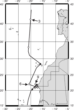
Here, we report iron stable isotope data for aerosol samples collected during the AMT15 cruise[20] (Southampton, UK to Cape Town, South Africa, September/October 2004) and aerosols collected at Barbados (Fig. 1). The Barbados samples were selected to represent relatively high dust periods with North Africa as the main dust source. We also determined the iron stable isotope composition of soil samples from Chinese and Australian deserts (Table 1).
|
|
For iron stable isotope analysis, aerosol and desert soil extracts were digested in the presence of H2O2 and concentrated HNO3 in order to dissolve samples and to ensure that all the Fe was oxidised to FeIII. The residues of evaporation were then redissolved in 7 M HCl for chromatographic Fe separation. Anion exchange chromatography was performed using BioRad AG1-X8 resin columns. After elution of the matrix elements with 4 M HCl, Fe was eluted with 0.04 M HCl. This separation of Fe has been tested using a multi-element standard solution (Merck VI) and the IRMM-014 iron isotopic reference solution. The extraction procedure is quantitative and does not induce fractionation between Fe isotopes. Subsequently the samples were evaporated and redissolved in 2% HNO3 for elemental and isotopic measurements.
The elemental concentration of Fe and possible interfering elements such as Ca (CaO), Cr and Ni were determined on an Agilent 7500c Quadrupole Inductively Coupled Plasma Mass Spectrometer (Q-ICPMS). Only samples with less than 0.1% contaminants relative to Fe were accepted for further processing.
The isotope ratio measurements were performed on a VGi Isoprobe Multi Collector Collision Cell Inductively Coupled Plasma Mass Spectrometer (MC-CC-ICPMS) with static measurement of iron isotopes 54Fe, 56Fe and 57Fe on the Faraday cups. The ArN interference was eliminated by the use of Ar and H2 in the collision cell. To correct for mass bias drift, the IRMM-014 iron isotopic reference solution, at the same concentration (within 5%) as the sample, was run between each sample and a linear mass fractionation correction was applied using the values of Rosman and Taylor.[21] Because of the very small Fe amounts in the samples, they were run in triplicate at 200 ng mL–1 if possible, or at least in duplicate. Only samples with an Fe concentration >500 times that of the procedural (digest plus column) blanks as determined on the Q-ICPMS were measured.
Results are reported in standard δ notation (parts per 103)[15]


The longer term accuracy during the half year of incidental measurements for this project of the IRMM-014 56Fe/54Fe and 57Fe/54Fe are ±0.1‰ and 0.16‰ (2sd) respectively. The precision of the sample results was determined from the duplicate and triplicate data on soil samples (i.e. the higher concentration samples, since for other samples there was insufficient sample) as ±0.1‰. We subsequently report results to two decimal places to avoid having to often round uncertainties to ±0.0. Two samples out of 31 gave highly anomalous fractionations, which we assume represent contamination and are excluded from subsequent analysis.
Both δ56Fe and δ57Fe were determined in order to assess the quality of the separation and measurements. Even within the narrow range of values measured here, the two isotope ratios were highly correlated (r = 0.77, n = 29) with a slope of 2.06 (δ57Fe/δ56Fe), which is very close to the theoretical mass dependent fractionation line.[15] For the subsequent discussion we focus on the δ56Fe, as it is the more accurate because of a higher abundance of 56Fe relative to 57Fe in the measurement and is less susceptible to interferences.
Global models of total dust deposition to the oceans show a huge range of fluxes from ~0.1 g m–2 yr–1 over much of the remote Southern Ocean to >50 g m–2 yr–1 off the coast of North West Africa. Our recent research,[6] using samples collected during Atlantic Ocean cruises, spanning more or less the entire global range of aerosol dust loadings, demonstrates that there is also a systematic inverse variation in aerosol iron solubility with atmospheric dust concentration and hence flux (Fig. 2). Jickells and Spokes[12] have considered factors that might control the solubility of aerosol iron. It is not possible from the data in Fig. 2 alone to deduce the mechanism that gives rise to this systematic variation in solubility, however, it is possible to consider the relative significance of several of the potential mechanisms proposed by Jickells and Spokes.[12]
|
Similar trends are seen for other elements of low solubility that are tightly bound to aluminosilicates such as Al and Si,[6] and hence the mechanism is not unique to Fe as might be the case if iron redox cycling were important. Other metals not so strongly associated with aluminosilicate lattices show quite different solubility patterns (e.g. Mn, Fig. 2). An alternate, or possibly parallel, mechanism for enhancing iron solubility and that of other aluminosilicate bound metals (but not Si) would be processing by acids during atmospheric transport. However, Baker et al.[18] report no correlations of iron solubility with acid availability in aerosols. A final possibility would be if, remote from desert regions, alternative and more soluble iron sources overwhelm dust sources, for instance anthropogenic or volcanic emissions.[1] Given that anthropogenic iron sources are likely to be predominantly in the Northern Hemisphere and that volcanic sources are likely to be distributed thinly but widely around the planet, it is difficult to equate the symmetric increase in iron solubility seen in low dust regions of both the northern and southern hemispheres with a significant role for non-dust sources of iron. There are no local variations in solubility related to proximity to volcanic islands along the Atlantic Meridional Transect (AMT). These considerations led Baker and Jickells[6] to conclude that the simplest hypothesis consistent with the Fe results in Fig. 1 is that during long-range transport, larger dust particles are systematically lost as a result of preferential wet and dry deposition to leave smaller aerosol particles with larger surface-to-volume ratios and that these are more soluble. Although this mechanism is essentially a physical one, it is possible that atmospheric chemical processing may contribute to changes in iron particle size distribution and hence solubility.
The range of solubility we observe is ~100 fold (0.5–50%). This range is considerably less than the range in aerosol concentration[6] or dust deposition,[1] but the solubility trend is opposite to the dust gradient and will act to reduce the overall gradient in soluble iron supply to the oceans. The main soluble iron inputs to the oceans will still be to the areas downwind of the major deserts where dust fluxes are greatest. Thus, in considering global iron budgets it is necessary to focus attention on such high dust deposition ocean regions, while in considering atmospheric inputs to HNLC regions such as the Southern Ocean, it is the local solubility that will be of particular significance.
The desert soil samples analysed (Table 1) had iron isotope compositions very close to 0 (0.08 ± 0.04, n = 8), which is consistent with other studies of contemporary soils and rocks.[14,15,22] Ammonium acetate extracts of two of the desert soils gave an average δ56Fe value of –0.06‰, which suggests that the labile iron fraction (as defined by our procedures) in desert soils is isotopically similar to the total iron fraction.
Both the AMT15 and Barbados aerosol samples were heavily influenced by African dust emissions.[23] The isotopic composition of total iron in both sample sets is similar for those samples analysed (δ56Fe = 0.04 ± 0.09, n = 4), which is consistent with the anticipated dominance of desert soils as an iron source and with the only other published data for aerosols.[14] The isotopic composition of the soluble iron extracts of the samples is essentially identical in both datasets (AMT15 0.12 ± 0.22, n = 6; Barbados 0.13 ± 0.11, n = 3) so we can merge the datasets to derive an average aerosol soluble iron isotopic signature of δ56Fe = 0.13 ± 0.18 (n = 9). This value is again essentially the same as that of crustal material. Although the Barbados and AMT aerosol samples represent periods of high dust loading, samples will still have been subject to several days to a week of atmospheric transport and associated biogeochemical processing before collection. This is particularly true of the Barbados samples collected some 4000-km away from the source region. The results suggest that over a timescale of a few days of atmospheric transport at least, there appears to be no significant isotopic fractionation of soluble iron from its parent crustal material as a result of atmospheric processing. Hence the isotopic composition of total and readily soluble iron entering the ocean from the atmosphere in high dust regions (which dominate the iron input to the oceans) is essentially zero and similar to crustal material. We were unable to measure reliable stable iron isotope data for aerosols collected from the southern hemisphere during AMT15 because of the very low iron content of those samples.
Our results demonstrate that both dust fluxes and dust iron solubility show very large and systematic gradients across the oceans. These gradients work to some extent to counteract each other, with the result that the relative differences in soluble iron fluxes between ocean regions are not as extreme as in total dust inputs. In evaluating regional and local iron budgets, it is important to consider the gradients in solubility as well as the total dust flux. On a global basis the main inputs of both soluble and total iron occur downwind of the main desert regions such as off North Africa and Asia where iron solubility is relatively low (Fig. 2), which is consistent with the inverse calculations of Jickells and Spokes.[12] Our results suggest that the isotopic signature of the soluble iron in such regions is essentially identical to that of the crustal/soil source material. Other isotopic signatures in aerosols such as Nd or Sr[24] and Pb[25] are more useful as tracers of aerosol sources and transport, but of course of much less biogeochemical significance within the ocean.
The impact of atmospherically delivered soluble iron on surface ocean biogeochemistry will depend on the nutrient status of the receiving waters, the balance of limiting nutrients in the water column[10,26] and the relative magnitude of atmospheric inputs of iron and other nutrients (N,P)[27] all of which vary regionally.
Our studies only define a soluble iron component from the aerosol. This cannot represent the full complexity of iron cycling in seawater where wet and dry deposited dust is processed in the surface mixed layer by a variety of biogeochemical processes, which include complexation by strong organic ligands and direct interactions with bacteria, phytoplankton and zooplankton over timescales of many tens of days.[1] No simple chemical extraction can hope to mirror the complexity of these interactions. Boyd et al. quantified this complexity during the FeCycle field campaign, and showed an intense cycling of iron within the euphotic zone. It was also shown that, although inputs and export of iron within the euphotic zone were approximately in balance, the form of the iron was transformed during passage through the euphotic zone from primarily aluminosilicate in the atmospheric input to primarily biogenic in the sinking flux from the euphotic zone. Unravelling the complex biogeochemical cycling within the euphotic zone represents a major challenge for the future.
Acknowledgements
This work was supported by NERC grant NER/B/S/2003/00780 and sampling was supported by the AMT programme under NERC grant NER/O/S/2001/00680/01244. We acknowledge Carol Robinson’s leadership of AMT and Andy Rees as PSO of AMT15. This is contribution 155 of the AMT programme. We thank Doug Mackie and J.J. Cao for providing desert soil samples and Joe Prospero for providing the Barbados aerosol samples. We also thank two referees for their helpful comments.
[1]
T. D. Jickells,
Z. S. An,
K. K. Anderson,
A. R. Baker,
G. Bergametti,
N. Brooks,
J. J. Cao,
P. W. Boyd,
R. A. Duce,
K. A. Hunter,
H. Kawahata,
N. Kubilay,
J. La Roche,
P. S. Liss,
N. Mahowald,
J. M. Prospero,
A. J. Ridgwell,
I. Tegen,
R. Torres,
Science 2005, 308, 67.
| Crossref | GoogleScholarGoogle Scholar |
| Crossref | GoogleScholarGoogle Scholar |
| Crossref | GoogleScholarGoogle Scholar |
| Crossref | GoogleScholarGoogle Scholar |
| Crossref | GoogleScholarGoogle Scholar |
| Crossref | GoogleScholarGoogle Scholar |
| Crossref | GoogleScholarGoogle Scholar |
| Crossref | GoogleScholarGoogle Scholar |
| Crossref | GoogleScholarGoogle Scholar |
| Crossref | GoogleScholarGoogle Scholar |
| Crossref | GoogleScholarGoogle Scholar |
| Crossref | GoogleScholarGoogle Scholar |
| Crossref | GoogleScholarGoogle Scholar |
| Crossref | GoogleScholarGoogle Scholar |
| Crossref | GoogleScholarGoogle Scholar |
| Crossref | GoogleScholarGoogle Scholar |
| Crossref | GoogleScholarGoogle Scholar |
| Crossref | GoogleScholarGoogle Scholar |
| Crossref | GoogleScholarGoogle Scholar |
| Crossref | GoogleScholarGoogle Scholar |
| Crossref | GoogleScholarGoogle Scholar |
| Crossref | GoogleScholarGoogle Scholar |
| Crossref | GoogleScholarGoogle Scholar |
| Crossref | GoogleScholarGoogle Scholar |
