

Precipitation Isotopes New Zealand (PINZ): improvements in precipitation isoscapes with machine learning
A. F. Hill A , A. McKenzie B , B. D. Dudley B * and D. B. Nelson C
A
B
C
Abstract
Stable water isotopes δ18O and δ2H in atmospheric precipitation are valuable hydrologic tracers with varied applications, but measuring them over large scales is impractical. Precipitation isotope models (isoscapes) are instead needed to predict isotopes through space and time. Precipitation isotopes are affected by numerous variables ranging from orographic effects to phase changes to moisture mass origin, making them challenging to predict in complex geographies such as New Zealand. Improving data density together with recent advances in modelling approaches hold promise for improving accuracy of precipitation isoscapes in New Zealand and similar locations.
Precipitation isotope models based on global networks, such as the Global Network of Isotopes in Precipitation (GNIP), lack sufficient spatial and temporal resolution for hydrological applications in New Zealand due to sparse data coverage. Models driven by regional datasets are needed to improve accuracy of isotope predictions to increase utility in environmental research applications.
We develop Precipitation Isotopes New Zealand (PINZ) δ18O and δ2H isoscapes employing the Extreme Gradient Boosting (XGBoost) machine learning algorithm driven by a regional precipitation isotope database with high station density across New Zealand, and diverse climate and geographic predictors. We produce a national monthly precipitation isotope model at 5-km resolution. Model uncertainty associated with monthly predictions is evaluated using ‘leave one out’ cross validation (LOOCV, or jackknife) tests.
PINZ shows significant spatial and temporal variability in isotope values, with notable patterns related to New Zealand’s complex topography and climatic influences. Model performance on test data is described by a root mean square error of 1.83‰.
Although the model performs well overall, it exhibits limitations in predicting extreme precipitation δ18O values (most enriched and most depleted) and predicting δ18O of precipitation during periods of extreme weather conditions. Leveraging detailed local data and advanced algorithms, we demonstrate one way forward for improving isoscapes in complex environments.
Keywords: isoscape, isotope hydrology, machine learning, monthly isoscape, New Zealand, oxygen and hydrogen stable isotopes, precipitation isotope model, tree boosting algorithm.
Introduction
Isotopes of water provide a window into otherwise invisible aspects of the water cycle such as transit times through catchments (Jasechko 2019; Benettin et al. 2022), origins of streamflow (Liu et al. 2004; Hill et al. 2020) and evaporation processes (Kirchner and Allen 2020; Gibson et al. 2021; Vystavna et al. 2021). Understanding patterns of isotopes across the hydrological cycle can also provide insight into the origins of geological and biological materials that incorporate oxygen and hydrogen from water, with applications across a wide range of scientific fields including ecohydrology, anthropology, forensics, ecology and paleoclimatology (West et al. 2006; Lachniet 2009; Bartelink and Chesson 2019; Guerrieri et al. 2019). In New Zealand, stable water isotopes have been employed in a variety of applications and timescales. For example, improving knowledge of seasonally varying precipitation processes (Purdie et al. 2010; Kerr et al. 2015; Yang et al. 2020), determining groundwater sources and residence times on the order of years to decades (Stewart et al. 2007), and in paleoclimate reconstructions looking back over millennia (Lorrey et al. 2018).
Some of these applications are limited by accurate representation of stable water isotopes of hydrogen and oxygen (hereafter δ2H and δ18O) in precipitation. Accurate characterisation of stable isotopes in precipitation is often impractical by measurement of samples, especially for large scale studies, for catchments that extend to high elevations or for historical time periods. For such applications, it can be advantageous to use modelled precipitation isotope datasets (Lin et al. 2022; Stadnyk and Holmes 2023). However, modelled data products are only useful if they are appropriately accurate for the application. Global modelled spatial isotope surfaces (hereafter ‘isoscapes’) that predict isotopes at a given location and time (Bowen and Revenaugh 2003; Allen et al. 2019; Terzer-Wassmuth et al. 2021) do not offer sufficient spatial and temporal accuracy for most local environmental applications within New Zealand. Data for global models are commonly sourced from the International Atomic Energy Agency’s (IAEA) Global Network of Isotopes in Precipitation (GNIP), and other northern hemisphere precipitation networks. For New Zealand, the GNIP network is not representative of precipitation isotopes on a national scale: there are two GNIP sites with long-term data series, one each at extreme high and low latitudes and both at sea level. These sites miss critical influencing factors on New Zealand’s precipitation isotopes (Baisden et al. 2016). Regional isoscape development may improve predictions if they use more local data and specific statistical predictors relevant to the region, especially for regression-based approaches (Allen et al. 2019).
A regional precipitation isoscape for New Zealand is especially challenging given the diversity of New Zealand’s topography and climate. New Zealand’s island location and long, narrow shape (traversing 12° latitude) in the Southern Ocean means it receives moisture laden air masses that originate from all directions spanning cold southerlies from Antarctica to warm, humid systems brought by the sub-tropical ridge (Salinger 1980). Storms include regular atmospheric river events that bring high-intensity, multi-day rainfall (Prince et al. 2021). The prow of the Southern Alps mountain range that runs the length of the South Island of New Zealand produces strong orographic precipitation effects that are most dramatic from west to east where the land rises at an average 12% gradient from the west coast to New Zealand’s highest point, before a rain shadow dominates the eastern plains. Some temporal variation in rainfall isotope values across New Zealand can be accounted for with seasonal models (Dudley et al. 2024), however, much of the temporal variation across New Zealand is non-seasonal and associated with moisture origin – this is particularly the case in windward areas and those with maritime climates, whereas temperature-driven seasonal patterns are more pronounced in the central east (Stewart and McDonnell 1991; Baisden et al. 2016; Dudley et al. 2018; Marttila et al. 2018).
These examples of interacting, temporally variable climate factors demonstrate the complexity of relationships between predictors that are difficult to quantify and replicate statistically in commonly used multi-variate linear regression models (West et al. 2009). When the goal is to predict precipitation isotope values most accurately instead of disentangling mechanisms affecting precipitation isotope change, it is likely that the modelling task is better suited to data-intensive machine learning (ML) approaches (Nelson et al. 2021). ML models are appropriate for such complex tasks because of their ability to integrate non-linear interactions between variables that are otherwise challenging to prescribe. Here we present monthly oxygen (δ18O) and hydrogen (δ2H) isoscapes developed through XGBoost (Extreme Gradient Boosting, Chen 2016), a parallel tree boosting ML algorithm, to produce a publicly available continuous monthly precipitation isotope model for New Zealand from 2004 onwards at 5-km resolution. δ18O isoscapes are presented in detail in the body of this paper, whereas δ2H isoscapes are provided as Supplementary material. This work demonstrates that in complex geographies with myriad isotope-influencing and interacting processes, a ML modelling approach is a way forward for improving prediction of precipitation isotopes that can be replicated in other regions of the world.
Methods
Isotope notation
Stable isotope change processes in hydrology refer to the variation in the ratios of isotopes such as oxygen-18 and deuterium in water as it undergoes processes such as evaporation, condensation and infiltration. Stable isotope composition refers to the relative abundance of different isotopes in a sample. We refer to stable isotope composition in the delta (δ) notation, expressed as a deviation in parts per 1000 (i.e. ‘permille’, ‰), as a relative measure of isotope enrichment or depletion compared to the standard:
where Rsample and Rstandard are the ratios of the heavy to light isotope (e.g. or ) in the sample and the internationally recognised standard respectively. For both oxygen and hydrogen isotopes in water, the standard is Vienna Standard Mean Ocean Water (VSMOW), and the reference isotope scale is defined by this, as well as Standard Light Antarctic Precipitation (SLAP) (International Atomic Energy Agency 2021).
Data sources
Compared to traditional regression-based approaches, ML model capabilities rely on increased data requirements beyond those that have been historically available for New Zealand. To overcome this data shortfall and enable use of ML, we used existing precipitation networks and established an additional data collection network in 2021 that targeted sites to characterise isotope processes that were previously poorly represented in historical datasets (Fig. 1). New data collection was focused on high elevation sites and transects to capture west–east orographic effects (Supplementary Fig. S1 and S2).
Sample sites and associated number of observations for 2005 onwards. The black circle on the southern coast of the South Island represents the GNIP-Invercargill site that has 228 observations since 2005 (this site is not represented by colour or dot size due to scale).
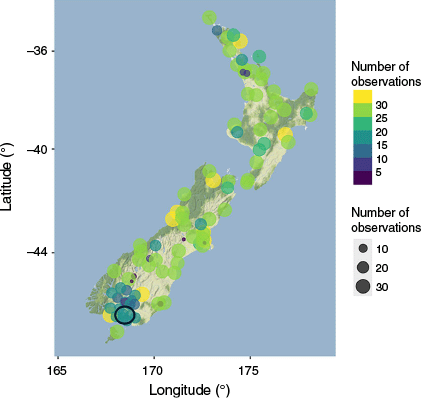
The dataset compiled existing records from sites across New Zealand (Supplementary Fig. S1) including those previously collected through National Institute of Water and Atmospheric research (NIWA) research, newly collected samples at NIWA Snow and Ice Network sites, by researchers (most notably a dataset collected at 54 sites over 2007–09 as per Baisden et al. 2016), various sampling efforts from local government scientists, and as part of the global IAEA Global Network of Isotopes in Precipitation (GNIP) network at two sites (Invercargill and Kaitaia). For the available precipitation isotope data, 13.83% of it was from prior to 1992 and only from two GNIP sites, with no data from 1992 to 2004 (inclusive). To mitigate the disproportionate impact of the GNIP sites on the geographic distribution of data and on the model, as well as to ensure the model is representative of recent climate conditions relevant to contemporary science applications, we limited the historical data record used to 2005 onwards.
Previous studies highlighted specific data gaps in New Zealand’s available precipitation isotope records (Kerr 2013; Dudley et al. 2024) that in part result in less accurate model predictions in the mountainous regions of New Zealand. To better capture the orographic effect on precipitation isotopes we installed two sampling transects across the Southern Alps in 2021 that generated 2 years of weekly or monthly precipitation samples (Supplementary Fig. S2). Also, in 2021 we launched a citizen science program mostly aimed at alpine professionals. Climbers and skiers across New Zealand sourced 121 unique high-elevation solid precipitation samples, including from the summits of New Zealand’s highest peaks, that were used to evaluate model performance. Four ski areas contributed weekly winter samples. Sites that were sampled weekly were aggregated to monthly by a volume-weighted average calculation. In rare cases where weekly volumes were unavailable, weekly samples were averaged for the month.
The total number of monthly precipitation isotope samples used to create PINZ is 2499 samples over 98 unique sites across New Zealand (Fig. 1) between 2005 and 2024. Because the dataset is a compilation of available historical data and newly collected samples, samples were analysed for δ18O and δ2H across several facilities. Details of the analyses can be found in Supplementary Table S1.
Model predictors include 3 geographic and 11 climate variables (Table 1) and month. Climate data were sourced from NIWA’s Virtual Climate Station Network (VCSN) (Tait et al. 2006, 2012; Tait and Woods 2007). VCSN produces daily climate data on a 5-km grid interpolated from measurements at climate stations across New Zealand. All predictor data were normalised to improve computational stability. We used minimum and maximum daily temperatures interpolated using the Norton method (Tmin_N, Tmax_N) instead of the operational VCSN temperature interpolation method. Norton interpolation corrects the warm bias in high mountainous terrain (>1000 m above sea level, ASL) without compromising accuracy of low elevation estimates (Tait and Macara 2014). Geographic variables include latitude, longitude and elevation from the R package elevatR (ver. 0.99.0, see https://github.com/jhollist/elevatr/; Hollister et al. 2023). Month was also retained as a predictor given seasonality of precipitation isotopes (Dudley et al. 2024) and was put in as a dummy variable using one-hot encoding. The monthly isotope measurements at each site were paired in time and location with the VCSN database. The daily VCSN climate data were reduced to monthly mean values at each site to match the measured isotope data timescale. Although we acknowledge that other land cover and atmospheric circulation variables may have provided additional predictive power to the model, we chose to limit our predictor set to this suite of 14 variables to simplify the model inputs to those used by previous New Zealand precipitation isotope modelling efforts for best comparison across approaches.
| Parameter | ||
|---|---|---|
| Tmin_N | Minimum temperature using the Norton method | |
| Tmax_N | Maximum temperature using the Norton method | |
| ETmp | Earth temperature at 10-cm depth | |
| Rad | Solar radiation | |
| MSLP | Mean sea level pressure | |
| PET | Potential evapotranspiration | |
| Rain_bc | Rainfall with bias correction | |
| Wind | Average wind speed at 10 m above ground level (2005 onwards) | |
| SoilM | Soil moisture | |
| RH | Relative humidity | |
| VP | Vapour pressure | |
Model structure
We modelled precipitation δ18O and δ2H values using a suite of climate and geographic predictors using XGBoost, a tree-based ML modelling approach built on gradient boosting algorithms. It develops an ensemble of decision trees and is built sequentially, where each new tree corrects errors made by the combination of previously grown trees. The XGBoost model was run within the Tidymodels framework (ver. 1.3.0, M. Kuhn and H. Wickham, see https://cran.r-project.org/package=tidymodels or https://www.tidymodels.org) in R (R Foundation for Statistical Computing, Vienna, Austria, see https://www.r-project.org/) using the boost_tree function and the XGBoost engine. The number of trees was set at 1000 and the hyperparameters min_n, tree_depth, learn_rate and loss_reduction for the boosted regression tree model were estimated by a five-fold cross validation on a grid of size 60 defined by the grid_max_entropy function. The number of trees is strongly correlated with the other hyperparameters, particularly the learning rate, and was set at a value of 1000 based on the dataset complexity, in order to constrain the estimation of the other hyperparameters during tuning. The choice of the number of trees was also checked by assessing the learning curve, which shows the change in model error in the training and validation data with each additional tree. Initially, this drops quickly with each added tree, but then eventually reaches a plateau of diminishing returns. The number of trees (n = 1000) was confirmed to reach this plateau, while making sure not to add too many, which would be identified through declining model performance (larger error) in the validation data after too many trees were included. The exact number is somewhat arbitrary, provided it falls within the optimal fit range on the learning curves. The final model was fitted using the XGBoost engine with parameters estimated by minimising the squared error.
Given a set of predictor data, this method generates precipitation isotope predictions using the trained XGBoost model. A user-defined loss function (we used the default regression with squared loss) measures the accuracy of the model’s predictions.
Our PINZ ML model was developed using precipitation isotope data collected from 2005 onward, as discussed above. The data were split into training data (80%) and test data (20%). The split was done within isotope quartile strata, then pooled, which ensured that there were similar isotope distributions for the training and test data sets.
Predictor variable importance
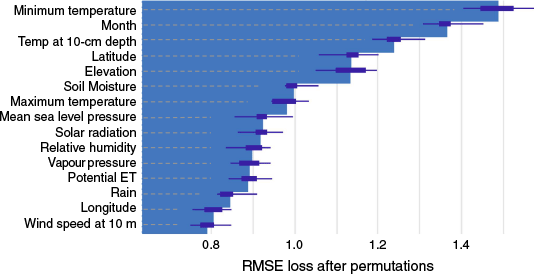
A helpful aspect of a tree-based algorithm model infrastructure such as XGBoost is global feature importance (GFI). GFI evaluates the relative importance of predictor variables by permutating the values for a predictor variable and evaluating the impact on model performance (i.e. isotope prediction). If permutating the predictor values makes little difference to model performance, the predictor variable is then reasonably unimportant. GFI not only assists in understanding which temporal, climate and geographic variables are most influential, it can also allude to inconspicuous mechanistic processes or interactions that affect precipitation isotope variability that would otherwise go unnoticed, and, in this way, GFI has the potential to provide new insights to the field of isotope change processes.
Model tuning
For the final model we used the best hyperparameter values assessed using the root mean square error (RMSE) criterion (Table 2), with all other parameters set to the default.
| Parameter | Definition | Default parameter value | Final model parameter | |
|---|---|---|---|---|
| min_n | An integer for the minimum number of data points in a node required for it to be split further. | 5 | 14 | |
| tree_depth | An integer for the maximum depth of the tree (i.e. number of splits) (specific engines only). | 6 | 13 | |
| learn_rate | A number for the rate at which the boosting algorithm adapts from iteration to iteration (shrinkage parameter). | 0.3 | 0.0107162 | |
| loss_reduction | A number for the reduction in the loss function required to split further. | 0 | 6.13 × 10⁻¹³ |
Model performance
We assessed model performance by comparing model predictions with the associated observations using the test data (20% of data set), training data (80% of data set) and all data combined. We report RMSE as our primary metric to evaluate the accuracy of the model.
Uncertainty in spatial predictions over New Zealand
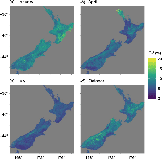
We evaluated model uncertainty associated with monthly predictions using ‘leave one out’ cross validation (LOOCV, or jackknife) tests (Hastie et al. 2009). For this analysis we constrained the period of prediction to months within the 2023 year. We conducted LOOCV to generate δ18O predictions for each of the 98 sites and 12 months. Using the training data we re-trained and ran the model 98 times, each time one site was dropped yielding a prediction across the 5-km grid based on the input data from the other 97 sites. This yielded a ‘stack’ of 98 model predictions at each grid point across New Zealand. We calculated mean, standard deviation and coefficient of variation (CV) statistics on the range of predictions at each VCSN grid point (98 predictions for each site) and month, producing a spatial representation of the CV of model predictions.
Results
Model performance
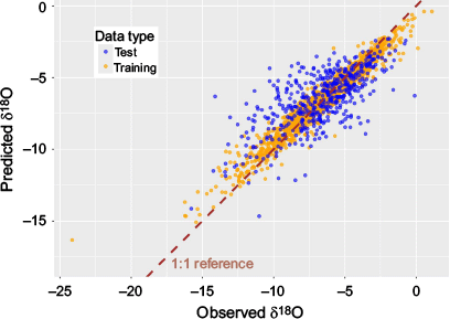
Model performance was evaluated using the 20% of test data set aside from the original dataset within δ18O quartile strata to ensure representative distribution of data in the test set. RMSE was used to evaluate the model performance at each site, with no clear spatial patterns across New Zealand (Fig. 2). The RSME for the overall model (national scale) evaluated using the test data is 1.83‰, evaluated on the training data is 0.64‰, and evaluated on all data is 1.00‰.
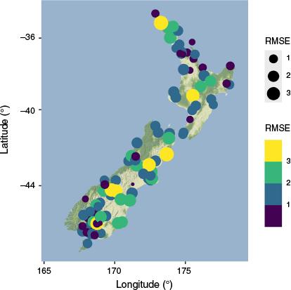
The sites with the highest RMSE occurred in contrasting geographies: RMSE = 3.76‰ (Frew 34), RMSE = 3.78‰ (Te Hiku) and RMSE = 3.25‰ (Ohau skifield). Ohau skifield is in the alpine, has samples limited to winter ski seasons, and is mainly comprised of solid precipitation (snow) samples. It also registered the lowest isotope value recorded in the dataset (δ18O = −24.14‰) during a short, severe cold snap in July 2021. Frew 34 is located on the north-east coast of the South Island near Kaikoura (25 m ASL), and the forested Te Hiku (RMSE = 3.78‰) is in Northland at 34 m ASL and was sampled during an especially unsettled period, discussed in more detail below.
Although R2 is a less helpful model evaluation metric than RMSE or mean absolute deviation (MAD), we report it here for clear comparison to previous modelling efforts. The model’s performance on the test data is summarised by a R2 of 0.54, and a R2 of 0.71 was achieved when assessing with all sample data.
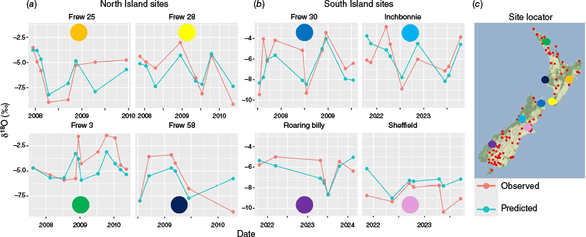
Time series predictions at sampling sites show the model’s capability to track sinusoidal seasonal cycles and generally capture the directions, if not the extent, of the extreme precipitation isotope signals (Fig. 3).
Model predictions as compared to test data observations on the (a) North Island and (b) South Island where Inchbonnie and Sheffield represent sites on the western and eastern side of the main divide respectively. (c) Colour-coded site locations shown are at representative, geographically distributed sites across New Zealand. Small red dots represent all sample sites.
Isoscapes
National monthly isoscapes at 5-km-grid resolution across New Zealand (Fig. 4) demonstrate both seasonal and non-seasonal spatial variation throughout New Zealand. Seasonality appears to be strongest in the lee of the central mountain ranges on both islands, whereas coastal areas demonstrate higher variability at sub-seasonal time scales. Here we present results for δ18O. δ2H isoscapes are provided in Supplementary Fig. S3 and S4.
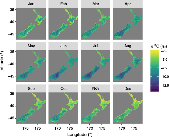
Across all months and seasons, the southern regions of the South Island in the rain shadow of the Southern Alps exhibit the most 18O-depleted (most negative) isotope values, whereas the coastal areas of the North Island are the most 18O-enriched (least negative). As expected, the colder winter period (June–August) receives the lowest isotopes across all regions as compared to the warmer months (December–February).
The influence of the South Island’s Southern Alps mountain range on the isotope progression from the west coast to the continental divide generally mimics the topography. However, the location of the lowest values from the summer and spring exhibit a geographical shift towards the east as summer–spring progresses to winter (e.g. February as compared to August in Fig. 4).
On the North Island, isotope values on the East Cape (north-eastern corner) follow the elevation changes associated with the Kaimanawa Range as compared to the more subdued coastal topography of the western coast of the North Island at similar latitudes. The higher elevation Central Plateau, home to the dominant Mount Ruapehu volcano, consistently displays lower isotopes across all months. The influence of other smaller ranges on the North Island to deplete (lower) isotopes is also apparent at the conical Mount Taranaki volcano on the south-west corner and the Tararua range north of Wellington.
Model prediction–observation comparison
The model shows a strong correlation between the predicted values generated by the model and the actual observed values in the dataset. Predictions plotted with the full observation dataset (all test and training data) (Fig. 5) result in a Pearson correlation coefficient of 0.71, signifying a strong positive linear relationship between what the model predicts and what actually occurs. The model is least accurate at predicting the high and low extremes of δ18O values. For values of δ18O less than −10‰ (i.e. more negative) the model tends to over-predict (prediction is a value higher than observed). For values greater than ~−2.5‰ (i.e. closer to zero) the model tends to underpredict (predicts a value lower than observed) – this pattern is observed both at the national and site level.
Predictor importance
The GFI (explained in detail in the ‘Predictor variable importance’ section above) chart indicates minimum daily temperature (Tmin_N), month and earth temperature at 10-cm depth (ETmp) as the most important model predictors (Fig. 6). Latitude and elevation are next most important. Whereas vapour pressure (VP) is highly correlated with δ18O and the temperature-related variables that are powerful PINZ predictors (Tmin_N, Tmax_N and ETmp) (Supplementary Fig. S5), VP is absent from the top predictors in the GFI. Overlapping confidence intervals in the GFI, for example, for minimum daily temperature and month, demonstrate the range in importance of predictor variables, introducing challenges in assessing one predictor as clearly more important that the other. Additionally, the potential for non-linear interactions captured by the model to affect the influence of predictor variables is not obvious from variable-to-variable correlations (Supplementary Fig. S5).
Uncertainty in spatial predictions over New Zealand
The CV for δ18O predictions calculated using LOOCV demonstrate high variation at the highest elevations of the South Island’s Southern Alps across all seasons, and in the Northeast Cape in spring, summer and autumn (Fig. 7). Higher variability is generally observed in the summer as compared to the winter. This may be in part due to the lower absolute value of δ18O (i.e. closer to 0) in summer than in winter, leading to a higher CV when the standard deviation of the cross-validation results is divided by the mean.
Coefficient of variation (CV) for δ18O predictions across 4 months generally representative of New Zealand’s seasons in 2023: (a) January, (b) April, (c) July and (d) October. The figure shows data for 11,491 VCSN climate grid points in New Zealand, excluding points in the far north with CVs exceeding 20% for April.
Discussion
We tested XGBoost’s ability to model precipitation isotopes in the complex environment of New Zealand using a set of selected climate and geographic predictors, and thus if the model’s architecture can capture multifaceted interactions between climatic and topographic factors to improve prediction accuracy. Applying the XGBoost methodology to New Zealand provided improved accuracy to monthly isotope predictions over previous models, especially in coastal regions where much of the temporal variation is not seasonal (Dudley et al. 2024) but still important to capture for ecological and hydrological applications using precipitation isotopes.
Previous modelling studies at the national New Zealand scale include the initial regression-based approach by Baisden et al. (2016) and a sinusoidal model that models the seasonal and spatial variation of precipitation isotopes across New Zealand (Dudley et al. 2024). These two efforts, as well as PINZ, utilise VCSN climate variable predictors and the sample measurements from Baisden et al. (2016).
Baisden et al. (2016) produced mean annual and mean monthly isoscapes for New Zealand using a multi-linear regression modelling approach yielding R2 = 0.46 and RMSE = 1.9‰ for monthly δ18O predictions. We improved upon this work by augmenting the dataset including filling spatial data gaps at high elevations and across the Southern Alps to better capture the complex processes occurring as precipitation moves over major topography and throughout seasonal cycles. We were also able to leverage existing ML models that were not available until recently. Using all sample data (test and training data inclusive) to match the Baisden et al. (2016) evaluation approach, PINZ resulted in R2 = 0.71 and RMSE = 0.996‰ for monthly δ18O predictions.
Dudley et al. (2024) modelled precipitation isotopes over New Zealand using a sinusoidal modelling approach with the goal of capturing their seasonal swing (amplitude of the sinusoid) and the annual mean isotope value (offset). The basic premise of the sinusoidal model is that it uses its cyclical nature to capture seasonal signals. By design the sinusoidal model does not aim to capture non-seasonal temporal variation (event-based and inter-annual variability), which is very important in some areas of New Zealand and the globe (Allen et al. 2019). PINZ complements the sinusoidal approach by considerably improving our ability to describe spatial patterns and the extent of non-seasonal (e.g. event-based or inter-annual) precipitation isotope variation.
In both of these previous modelling efforts, the dataset used lacked measurements above 1291 m and only 3 of 58 sites were above 700 m. Much of New Zealand’s precipitation falls at elevations poorly represented by the dataset, yet elevation is commonly used as a predictor in the models, meaning that elevational trends from low-lying regions needed to be extrapolated to make predictions at higher locations. The accuracy of isotope prediction in the higher mountain areas was a shortfall that we were able to improve upon with PINZ’s expanded input data. Previous models might also be expected to perform better with more data, but the added complexity of environmental processes in the mountainous terrain from which the new data were drawn might also conversely result in decreased model performance from these previous approaches.
A central modelling limitation relates to the factors or predictors that were not incorporated into the model. The foundation of this modelling exercise is to predict precipitation δ18O values based on variables representative of the prediction site. Yet, it is well documented that precipitation δ18O values can be strongly related to upstream transport processes that deliver the moisture to the site of precipitation and to conditions at the evaporation source. No point-based model that does not incorporate transport processes can hope to perfectly capture these effects. However, on-site climate conditions may also be more preferentially associated with different types of transport modes, such that cool–wet conditions may generally be associated with moisture with one source, whereas warm–wet conditions are associated with another. By incorporating multiple climate and geographical predictors, such as those used in PINZ (e.g. latitude, mean sea level pressure), some such circulation patterns might be partially characterised, but they can never be fully accounted for without a much more complicated model. This can explain why this approach gives improved results over other point-based models but also does not perfectly replicate the δ18O values.
A longstanding challenge of modelling precipitation isotopes at scale is the spatiotemporal mismatch between samples and climate data. Precipitation isotope sampling time series are typically collected as monthly (or at best weekly) intervals, resulting in an aggregate isotope value that may attenuate isotope differences between climatically variable storms, including obscuring isotopic extremes. Alternatively, all of the precipitation in a given month could fall in one intense, cold event with the rest of the month being hot, so the mean temperature for that month will not reflect the conditions when that precipitation fell. One approach to manage this mismatch is to go to event-based sampling with high-resolution climate data. This approach has been applied for point-based studies seeking to understand a specific process or mechanism (Crawford et al. 2013), but it is not practical or even possible to do over a large region. This type of temporal mismatch is a good explanation for why a ML model like PINZ misses extreme values.
Much of the variation in precipitation δ18O that we observe across New Zealand can be explained by well-understood processes. For instance, the temperature dependence of the equilibrium isotope fractionation factor for oxygen governs the condensation reaction as precipitation forms, leading to lower δ18O values at higher elevations and latitudes (Friedman and O’Neil 1977). Furthermore, New Zealand’s long, narrow shape results in significant differences in precipitation isotope values across its length due to global atmospheric circulation and associated Rayleigh fractionation effects. A disproportionately large amount of atmospheric moisture is evaporated at the equator, and rainout effects result in progressive depletion in precipitation δ18O values as this moisture is transported poleward (Dansgaard 1964). However, in a modelling exercise such as PINZ, potentially complex interactions that effect precipitation isotopes can be unexpectedly highlighted. For example, we see in our model’s uncertainty analysis unusually high CVs in Northland in the mid-late austral summer of 2023 (Fig. 7b). The February–April 2023 period in Auckland and Northland experienced especially unsettled weather and this is uncharacteristic for this historically stable time of year: Cyclone Gabrielle made landfall in the region in mid-February 2023, followed by further heavy rain events and an atmospheric river event on 30 April 2023. These events are reflected in the extreme climate and precipitation isotope time series from February to April 2023 at the Te Hiku sampling site in Northland (Supplementary Fig. S6). Model performance will sharply drop off when climate predictors are outside the range of normal values, yielding higher variability in predictions when climate conditions (wind speeds, temperature, etc.) are outside the training parameter space, leading to an increase in CVs (Fig. 7b). Capturing of extreme conditions would improve model performance generally but requires a higher temporal resolution of data collection, as discussed above.
Further improvements to the model could include augmentation of predictor variables to represent moisture origin, atmospheric climate indices (e.g. El Niño–Southern Oscillation, ENSO), continentality, cloudiness, orography and land cover that may affect influential processes such as cloud formation, convection and moisture recycling. Representing moisture origin will always be a limitation with our current modelling approach but may be served by incorporating wind-related predictors (e.g. speed, direction). Potential approaches include wind rose data (local scale), wind back-trajectory analysis (regional scale) or zonal and meridional wind predictions (national scale) from numerical weather prediction (NWP) models. Downscaling reanalysis data from NWP models or Global Circulation Models to incorporate wind predictors at different atmospheric levels would go even further by incorporating larger atmospheric circulation.
ML approaches typically benefit from more data, especially to capture processes that fall outside historical norms or across multi-year cycles such as ENSO. Augmenting the PINZ dataset is straightforward, allowing for simple integration of small datasets into the sample data used to train and test the model. This allowed for incorporating a wider range of existing data and feasibility in acquiring increased data density in challenging-to-access locations by citizen scientists where a time series was not possible. For these reasons, PINZ is also well placed to receive additional sample data through outreach within the scientific communities. The vision for PINZ going forward is to transition to a community-based model structure that becomes a shared, open-source asset to the New Zealand isotope science community. This affords the opportunity to add both future data and legacy collections from within the community to the sample database used to train and test future iterations of the model, with the aim of continuing to improve both accuracy and utility of the precipitation isoscapes, especially in relation to better capturing extreme values or non-seasonal variations (e.g. circulation modes, significant storms).
Conclusion
We developed a machine learning model to create a publicly available national precipitation isoscape to predict δ18O and δ2H amid New Zealand’s complex geography and climate. We produce monthly isoscapes at 5-km spatial resolution. Compared to previous New Zealand isoscapes, PINZ improves accuracy of predictions, with the lowest accuracy predictions seen at the extreme isotope values. The model’s highest RMSE is observed in the higher elevation sites that have limited data, and in the far north at a site sampled during periods of prolonged unsettled weather conditions. The open access model structure is poised for continued development with the incorporation of additional data from the New Zealand isotope community, as well as with the inclusion of additional predictors, especially those that relate to moisture origin. The results from PINZ provide an example of how machine learning precipitation isotope models can be applied to other regions with complex environments to produce improved input datasets for a broad range of ecological, paleoclimate and hydrological applications.
Data availability
We provide free public access to PINZ model outputs for δ18O and δ2H, as well as access to precipitation isotope data used in model development. The PINZ model code in R programming language (ver. 4.4.2, R Foundation for Statistical Computing, Vienna, Austria, see https://www.r-project.org/) is also publicly available at https://github.com/niwa/PINZ.
Declaration of funding
A. F. Hill’s contributions were supported by a Rutherford Foundation Postdoctoral Fellowship from New Zealand Government funding, administered by the Royal Society Te Apārangi. Contributions of B. D. Dudley and A. McKenzie to this work were funded by New Zealand’s Ministry for Business, Innovation and Employment through the Endeavour Fund (under the Forest Flows programme led by Scion, contract number C04X1905) and the NIWA Strategic Science Investment Fund (SSIF). Funding sources provided essential time for the authors to complete the research and develop this manuscript under their research programs, but funding bodies had no such involvement in the decision to submit for publication.
Acknowledgements
The authors thank the many citizen scientists and regional council scientists who provided water collected from across New Zealand, and Russell Frew for providing access to much of the precipitation isotope data used in this study. Much appreciation goes to Travis Horton for assistance with timely isotope analysis of samples.
References
Allen ST, Jasechko S, Berghuijs WR, Welker JM, Goldsmith GR, Kirchner JW (2019) Global sinusoidal seasonality in precipitation isotopes. Hydrology and Earth System Sciences 23, 3423-3436.
| Crossref | Google Scholar |
Baisden WT, Keller ED, van Hale R, frew RD, Wassenaar LI (2016) Precipitation isoscapes for New Zealand: enhanced temporal detail using precipitation-weighted daily climatology. Isotopes in Environmental and Health Studies 52, 343-352.
| Crossref | Google Scholar | PubMed |
Bartelink EJ, Chesson LA (2019) Recent applications of isotope analysis to forensic anthropology. Forensic Sciences Research 4, 29-44.
| Crossref | Google Scholar | PubMed |
Benettin P, Rodriguez NB, Sprenger M, Kim M, Klaus J, Harman CJ, van der Velde Y, Hrachowitz M, Botter G, Mcguire KJ, Kirchner JW, Rinaldo A, Mcdonnell JJ (2022) Transit Time Estimation in Catchments: Recent Developments and Future Directions. Water Resources Research 58, e2022WR033096.
| Crossref | Google Scholar |
Bowen GJ, Revenaugh J (2003) Interpolating the isotopic composition of modern meteoric precipitation. Water Resources Research 39, 1299.
| Crossref | Google Scholar |
Chen TCG (2016) XGBoost: a scalable tree boosting system. In ‘KDD ‘16: Proceedings of the 22nd ACM SIGKDD International Conference on Knowledge Discovery and Data Mining’, 13–17 August 2016, San Francisco, CA, USA. (Eds B Krishnapuram, M Shah, ASmola, C Aggarwal, D Shen, R Rastogi) pp. 785–794. (Association for Computing Machinery: New York, NY, USA) 10.1145/2939672.2939785
Crawford J, Hughes CE, Parkes SD (2013) Is the isotopic composition of event based precipitation driven by moisture source or synoptic scale weather in the Sydney Basin, Australia? Journal of Hydrology 507, 213-226.
| Crossref | Google Scholar |
Dansgaard W (1964) Stable isotopes in precipitation. Tellus 16, 436-468.
| Crossref | Google Scholar |
Dudley BD, Marttila H, Graham SL, Evison R, Srinivasan M (2018) Water sources for woody shrubs on hillslopes: an investigation using isotopic and sapflow methods. Ecohydrology 11, e1926.
| Crossref | Google Scholar |
Dudley B, Hill A, Mckenzie A (2024) A seasonal precipitation isoscape for New Zealand. Journal of Hydrology: Regional Studies 52, 101711.
| Crossref | Google Scholar |
Friedman I, O’Neil JR (1977) Compilation of stable isotope fractionation factors of geochemical interest. Professional Paper 440-KK, US Geological Survey, US Department of the Interior. 10.3133/pp440KK
Gibson JJ, Holmes T, Stadnyk TA, Birks SJ, Eby P, Pietroniro A (2021) Isotopic constraints on water balance and evapotranspiration partitioning in gauged watersheds across Canada. Journal of Hydrology: Regional Studies 37, 100878.
| Crossref | Google Scholar |
Guerrieri R, Belmecheri S, Ollinger SV, Asbjornsen H, Jennings K, Xiao J, Stocker BD, Martin M, Hollinger DY, Bracho-Garrillo R (2019) Disentangling the role of photosynthesis and stomatal conductance on rising forest water-use efficiency. Proceedings of the National Academy of Sciences 116, 16909-16914.
| Crossref | Google Scholar | PubMed |
Hill AF, Rittger K, Dendup T, Tshering D, Painter TH (2020) How important is meltwater to the Chamkhar Chhu headwaters of the Brahmaputra River? Frontiers in Earth Science 8, 81.
| Crossref | Google Scholar |
Hollister J, Shah T, Nowosad J, Robitaille A, Beck M, Johnson M (2023) jhollist/elevatr: CRAN Release v0.99.0. Zenodo 2023, v0.99.0.
| Crossref | Google Scholar |
Jasechko S (2019) Global isotope hydrogeology―review. Reviews of Geophysics 57, 835-965.
| Crossref | Google Scholar |
Kerr T (2013) The contribution of snowmelt to the rivers of the South Island, New Zealand. Journal of Hydrology 52, 61-82.
| Google Scholar |
Kerr T, Srinivasan M, Rutherford J (2015) Stable water isotopes across a transect of the Southern Alps, New Zealand. Journal of Hydrometeorology 16, 702-715.
| Crossref | Google Scholar |
Kirchner JW, Allen ST (2020) Seasonal partitioning of precipitation between streamflow and evapotranspiration, inferred from end-member splitting analysis. Hydrology and Earth System Sciences 24, 17-39.
| Crossref | Google Scholar |
Lachniet MS (2009) Climatic and environmental controls on speleothem oxygen-isotope values. Quaternary Science Reviews 28, 412-432.
| Crossref | Google Scholar |
Lin W, Barbour MM, Song X (2022) Do changes in tree-ring δ18O indicate changes in stomatal conductance? New Phytologist 236, 803-808.
| Crossref | Google Scholar | PubMed |
Liu F, Williams MW, Caine N (2004) Source waters and flow paths in an alpine catchment, Colorado Front Range, United States. Water Resources Research 40, W09401.
| Crossref | Google Scholar |
Lorrey AM, Boswijk G, Hogg A, Palmer JG, Turney CS, Fowler AM, Ogden J, Woolley J-M (2018) The scientific value and potential of New Zealand swamp kauri. Quaternary Science Reviews 183, 124-139.
| Crossref | Google Scholar |
Marttila H, Dudley B, Graham S, Srinivasan M (2018) Does transpiration from invasive stream side willows dominate low‐flow conditions? An investigation using hydrometric and isotopic methods in a headwater catchment. Ecohydrology 11, e1930.
| Crossref | Google Scholar |
Nelson DB, Basler D, Kahmen A (2021) Precipitation isotope time series predictions from machine learning applied in Europe. Proceedings of the National Academy of Sciences 118, e2024107118.
| Crossref | Google Scholar | PubMed |
Prince HD, Cullen NJ, Gibson PB, Conway J, Kingston DG (2021) A climatology of atmospheric rivers in New Zealand. Journal of Climate 34, 4383-4402.
| Crossref | Google Scholar |
Purdie H, Bertler N, Mackintosh A, Baker J, Rhodes R (2010) Isotopic and elemental changes in winter snow accumulation on glaciers in the Southern Alps of New Zealand. Journal of Climate 23, 4737-4749.
| Crossref | Google Scholar |
Salinger MJ (1980) New Zealand climate: I. Precipitation patterns. Monthly Weather Review 108, 1892-1904.
| Crossref | Google Scholar |
Stadnyk TA, Holmes TL (2023) Large scale hydrologic and tracer aided modelling: a review. Journal of Hydrology 618, 129177.
| Crossref | Google Scholar |
Stewart MK, McDonnell JJ (1991) Modeling base flow soil water residence times from deuterium concentrations. Water Resources Research 27, 2681-2693.
| Crossref | Google Scholar |
Stewart MK, Mehlhorn J, Elliott S (2007) Hydrometric and natural tracer (oxygen‐18, silica, tritium and sulphur hexafluoride) evidence for a dominant groundwater contribution to Pukemanga Stream, New Zealand. Hydrological Processes: An International Journal 21, 3340-3356.
| Crossref | Google Scholar |
Tait A, Macara G (2014) Evaluation of interpolated daily temperature data for high elevation areas in New Zealand. Weather and Climate 34, 36-49.
| Crossref | Google Scholar |
Tait A, Woods R (2007) Spatial interpolation of daily potential evapotranspiration for New Zealand using a spline model. Journal of Hydrometeorology 8, 430-438.
| Crossref | Google Scholar |
Tait A, Henderson R, Turner R, Zheng X (2006) Thin plate smoothing spline interpolation of daily rainfall for New Zealand using a climatological rainfall surface. International Journal of Climatology: A Journal of the Royal Meteorological Society 26, 2097-2115.
| Crossref | Google Scholar |
Tait A, Sturman J, Clark M (2012) An assessment of the accuracy of interpolated daily rainfall for New Zealand. Journal of Hydrology 51, 25-44.
| Google Scholar |
Terzer-Wassmuth S, Wassenaar LI, Welker JM, Araguas-Araguas LJ (2021) Improved high-resolution global and regionalized isoscapes of δ18O, δ2H and d-excess in precipitation. Hydrological Processes 35(6), e14254.
| Crossref | Google Scholar |
Vystavna Y, Harjung A, Monteiro LR, Matiatos I, Wassenaar LI (2021) Stable isotopes in global lakes integrate catchment and climatic controls on evaporation. Nature Communications 12, 7224.
| Crossref | Google Scholar | PubMed |
West JB, Bowen GJ, Cerling TE, Ehleringer JR (2006) Stable isotopes as one of nature’s ecological recorders. Trends in Ecology & Evolution 21, 408-414.
| Crossref | Google Scholar | PubMed |
Yang J, Dudley BD, Montgomery K, Hodgetts W (2020) Characterizing spatial and temporal variation in 18O and 2H content of New Zealand river water for better understanding of hydrologic processes. Hydrological Processes 34, 5474-5488.
| Crossref | Google Scholar |