
Seasonal sea level forecasts for the Australian coast
Ryan M. Holmes A * , Grant A. Smith B and Claire M. Spillman B
A
B
Handling Editor: Andrea Taschetto
Abstract
Seasonal-to-interannual anomalies in coastal water levels, associated with climate drivers such as the El Niño–Southern Oscillation (ENSO) and other atmospheric and oceanographic processes, contribute to coastal sea level extremes by raising the baseline sea level on top of which storm surges and tides act. These anomalies are potentially predictable months in advance, information that could be used to construct an early warning system for coastal flooding hazards. With this aim in mind, we present a comprehensive skill assessment of Australian coastal sea level ensemble forecasts made with the Australian Bureau of Meteorology’s seasonal prediction system, ACCESS-S2, between 1 and 8 months into the future. ACCESS-S2 has skill on the Australian north and west coasts, where sea level anomalies associated with tropical climate drivers can reach ±20 cm. Inclusion of the impact of atmospheric surface pressure variations on sea level (the ‘inverse barometer’) as a post-processing step increases skill around most of the coast, particularly in the east. Forecast skill metrics that incorporate ensemble uncertainty information, such as the Continuous Ranked Probability Score and the Brier Skill Score for median, upper tercile and upper decile exceedances, show significant improvements over reference anomaly persistence or climatology forecasts. Forecast skill arises largely from ACCESS-S2’s ability to forecast ENSO and its connection to Australian sea level by oceanic teleconnections, with other modes of variability playing a minor role. These seasonal sea level forecasts will be used for probabilistic sea level products with various applications, including improving community resilience to coastal flooding hazards.
Keywords: coastal hazards, coastal inundation, El Niño–Southern Oscillation, forecast skill, inverse barometer, sea level, seasonal prediction, verification.
1.Introduction
Coastal inundation is an increasingly significant hazard for many communities around Australia, and is 1 of the 10 priority hazards being assessed by Australia’s first National Climate Risk Assessment (NCRA, Department of Climate Change, Energy, the Environment and Water 2024). The frequency and severity of coastal flooding are expected to increase with sea level rise under climate change (Cooley et al. 2022), necessitating adaptation measures to protect coastal communities and infrastructure (Mortensen et al. 2024). Although extreme flooding events often receive the most attention, the cumulative cost of regular minor or nuisance flooding (‘high tide flooding’) may be comparable to that of extreme events in many locations, especially as sea level rise raises the baseline water levels around which tides vary (Moftakhari et al. 2017). In addition to affecting coastal communities through property damage, loss of access and loss of life, sea level extremes can also affect coastal ecosystems. For example, low sea level events can expose coral reefs causing bleaching (e.g. Ampou et al. 2017; Brown et al. 2019) or lead to mangrove die-backs (e.g. Abhik et al. 2021).
Seasonal forecasts of coastal sea level made up to a year into the future can provide valuable information for environmental managers, emergency services, local councils and port operators to prepare for and mitigate the impacts of extremes. The Australian Bureau of Meteorology’s seasonal ensemble prediction system, the Australian Community Climate and Earth-System Simulator-Seasonal prediction system version 2 (ACCESS-S2, Hudson et al. 2017; Wedd et al. 2022) provides seasonal forecasts of global sea level up to 8 months into the future on a low-resolution 1/4° grid. Studies have demonstrated that ensemble seasonal prediction systems, including ACCESS-S2, have skill relative to climatological forecasts in predicting low-frequency sea level variations out to and beyond 6 months into the future throughout broad regions of the tropical open oceans (Miles et al. 2014; Widlansky et al. 2017, 2023; Long et al. 2021). Although the processes governing coastal sea level variability differ from those in the open ocean and require finer grid resolutions to resolve, several studies have demonstrated that such models may also have skill at forecasting sea level along the coast (e.g. on the shelf and at tide gauge locations) where the impacts of sea level extremes are more keenly felt (McIntosh et al. 2015; Long et al. 2021, 2023; Jacox et al. 2023). In this study, we further demonstrate the skill and potential utility of these forecasts through a detailed assessment of ACCESS-S2’s inshore sea level predictions for the Australian coast.
Variability in coastal sea level is driven by a wide range of processes including but not limited to tides, storm surges, coastal upwelling, coastal trapped waves (CTWs), mesoscale eddies and wave processes (setup and run-up, not considered here). These processes act on different time scales, vary in amplitude around the coastline and differ in their predictability (Woodworth et al. 2019). Around Australia, tidal variability is strongest in the north, particularly on the north-west shelf, and weakest in the south and south-west (green line in Fig. 1a, d). By contrast, the high-frequency residual (sea level minus the tide) is strongest along the south coast associated with storm surges and mid-latitude synoptic variability (orange line in Fig. 1a). These signals, beyond weather time scales of a few days, tend to propagate anti-clockwise around the Australian coast, associated with CTW dynamics (White et al. 2014). The mean seasonal cycle is another source of sea level variability, reaching a standard deviation of 10 cm in the north (green line in Fig. 1b), peaking in austral summer (December–February) and autumn (March–May, Barroso et al. 2024) and weakening to the south, where it peaks in austral winter (June–August).
Standard deviations of various components of the sea level signal at the ANCHORS tide gauges over the 1982–2018 period. Tide gauges are listed in anti-clockwise order with corresponding locations marked in the map (d). (a) Standard deviation of the tide, the monthly averaged residual (sea level minus the tide) and the daily averaged residual. The standard deviation of the tidal signal is computed from hourly time series using the UTide software package (see Section 2), which includes the annual and semi-annual tidal constituents (thus the residual does not include the seasonal cycle). (b) Standard deviation of the monthly residual, the seasonal cycle (computed from the monthly climatology of the tidal signal) and the monthly averaged inverse barometer (IB). (c) Ratio of the variances of the monthly averaged to the daily averaged residual (blue) and the monthly averaged IB to residual (orange). Also shown are the fraction of the monthly averaged sea level variance associated with ENSO (here, the Niño 3.4 index, N34(t)) and with SAM (using the Marshall 2003 index) from a multi-linear regression on these two indices. For N34(t), with multi-linear regression coefficient B, this is computed as var (B × N34) ÷ var(SLA), where var is the variance operator and SLA(t) is the total (monthly averaged) residual sea level. (d) The colour of the symbols indicates the standard deviation of the tide (green line, a).
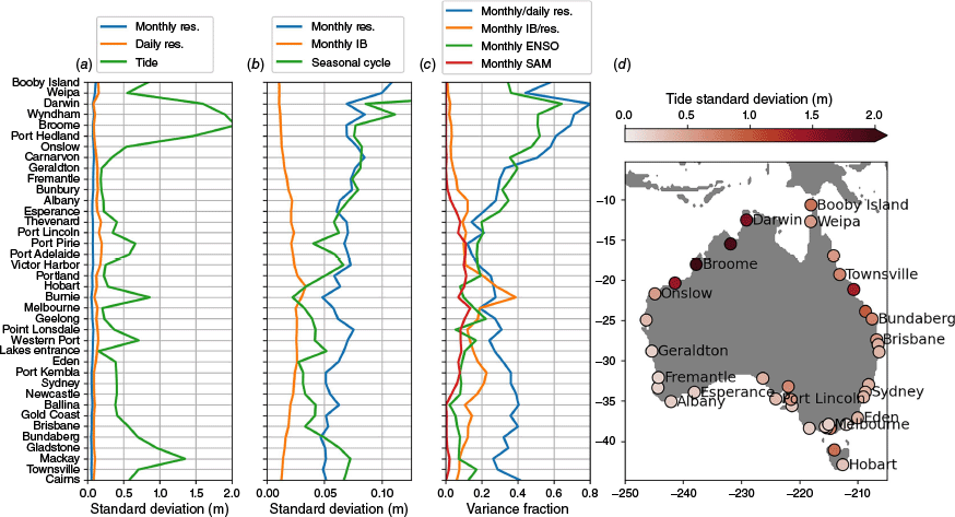
Of most interest for this study are the low-frequency (monthly) residual sea level anomalies (SLAs, from the mean seasonal cycle), as this is the signal, in addition to the high-frequency tides and mean seasonal cycle, that may be predictable on seasonal time scales. The low-frequency variability has an amplitude that decreases anticlockwise around the Australian coast (blue line in Fig. 1b, also see Middleton et al. 2007; White et al. 2014) and constitutes 15–80% of the total (daily) residual variability (blue line in Fig. 1c), highlighting the potential for seasonal predictions to provide useful information. Many of these low-frequency anomalies are associated with the El Niño-Southern Oscillation (ENSO), which, when characterised by sea surface temperature (SST) anomalies in the eastern Pacific Niño 3.4 region (5°N–5°S, 170–120°W), explains up to 60% of the variance on the north-west and west coasts (green line in Fig. 1c) due to oceanic teleconnections by CTWs (White et al. 2014). Lowe et al. (2021) showed that there was a 20% change in the 100-year extreme sea level event between El Niño and La Niña conditions in south-west Western Australia.
Other climate modes contribute to monthly sea level variability to a lesser extent. The Southern Annular Mode (SAM), corresponding to meridional shifts in the southern hemisphere westerly winds (Fogt and Marshall 2020), explains up to 15% of the variance along the south coast independently of ENSO (Fig. 1c). It has been demonstrated that the SAM has some predictability in ACCESS-S2 out to lead month 3, but only due to its connection to ENSO (Lim et al. 2013; Wedd et al. 2022). Other modes of seasonal climate variability, such as the Indian Ocean Dipole (IOD) or a second mode ENSO index (e.g. Frankcombe et al. 2015) have a relatively weak impact on Australian sea level when included in the multi-linear regression used to compute the variance fractions in Fig. 1c (not shown, also see Wang et al. 2021).
In addition to dynamic sea level variability, atmospheric sea level pressure variations (typically neglected in output from general circulation models) also drive variability in sea level through the ‘inverse barometer’ (IB) effect. On time scales beyond a few days, the IB can be approximated as follows:
where is the deviation of the sea level pressure from its global ocean mean, g is the acceleration due to gravity and ρs is the surface sea water density (we neglect the small variations in surface sea water density and take gρs = 9.9 mm hPa−1) (Ponte 1994; Gregory et al. 2019). Underneath strong, transient low pressure systems, the IB effect can often dominate the wind-driven dynamic impacts of the system on sea level (Ponte 1994). At longer time scales, the IB is smaller, but can still constitute a significant fraction of the total sea level variability. For Australia, monthly averaged IB anomalies are strongest along the south coast where they reach a standard deviation of ~4 cm (orange line in Fig. 1b) and account for 10–20% of the monthly residual sea level variance (orange line in Fig. 1c). The IB has been neglected in past studies of seasonal sea level predictability (e.g. Miles et al. 2014; McIntosh et al. 2015; Widlansky et al. 2023). However, the IB is indistinguishable from other components of sea level variability from a local impacts perspective. Thus, we consider it important to consider and, as suggested by Long et al. (2021), we explore the impact on forecast skill of adding the IB to the dynamic sea level in the ACCESS-S2 forecasts (yielding the total sea level) as a post-processing step.
In this paper we present a skill assessment of ACCESS-S2 seasonal coastal sea level forecasts up to 8 months into the future around the Australian coastline. We present both deterministic and probabilistic skill metrics and we assess the impact of adding the IB contribution to seasonal sea level, using ACCESS-S2’s sea level pressure forecasts. Finally, we provide a brief overview of the mechanisms responsible for predictability, and discuss the next steps required to operationalise these forecasts and maximise their utility for coastal decision makers.
2.Data and methods
2.1. Forecast model and hindcast experiments
The Australian Bureau of Meteorology’s seasonal ensemble prediction system, ACCESS-S2, is a coupled ocean–atmosphere model that provides subseasonal to seasonal forecasts for both atmospheric and oceanic climate variables at lead times out to 8 months. ACCESS-S2 is based on the UK MetOffice’s Global Coupled model GC2.0 (Williams et al. 2015). The ocean component is the Global Ocean GO5.0 (Nucleus for European Modelling of the Ocean, NEMO, ORCA25 Version 3.4, Madec et al. 2013; Megann et al. 2014) and is Boussinesq with a horizontal resolution of 1/4° and 75 vertical levels. The sea level does not include tides or explicitly capture the IB effect in the ACCESS-S2 instance (although the NEMO model code includes this option). The ACCESS-S2 prediction system is described in detail in Wedd et al. (2022).
In this article we utilise a set of hindcasts (retrospective forecasts) produced for the period 1982–2018 to assess model skill. We also provide a limited assessment of the performance of the ACCESS-S2 ocean reanalysis, from which the hindcasts are initialised (Wedd et al. 2022). The ACCESS-S2 ocean reanalysis assimilates in situ temperature and salinity data, as well as satellite SST data, whose assimilation will also constrain the model’s sea level variability. However, it does not assimilate satellite altimetry or tide gauge observations directly. For the skill assessment, we use a 27-member ensemble set available for the first day of each month in the hindcast period 1982–2018. This ensemble consists of a time-lagged set of three ensemble members initialised on the first day of the month and on each of the 8 days prior (including the last 8 days of 1981 for the 1 January 1982 ensemble), with the ensembles on each individual start date corresponding to a burst ensemble where small, semi-random perturbations are added to the prognostic atmospheric fields to represent initial condition uncertainty as described in more detail in Wedd et al. (2022) and Hudson et al. (2017). Hindcast simulations are run for 279 days, allowing us to construct full-member monthly forecasts for lead months 0–7, where month 0 indicates the forecast for the first month initialised on the first day of that month. Real-time forecasts, not considered here, have been run since 2018 and provide a time-lagged 99 member ensemble from daily simulations of 11 (perturbed) members from each of the past 9 days (Wedd et al. 2022). We consider the skill of both the ensemble mean (the mean of all ensemble members) forecast, as well as skill metrics that consider the ensemble spread, compared to various reference forecasts.
2.2. Observational data
We assess performance against the Australian National Collection of Homogenised Observations of Relative Sea Level (ANCHORS) tide gauge dataset (Hague et al. 2022), over the ACCESS-S2 hindcast period of 1982–2018. Hourly gauge data are first detided using the Utide software package (ver. 0.3.0, see https://pypi.org/project/UTide/), using 68 tidal constituents, applied over the full 1982–2018 time period and using no data filling. The hourly residual is then averaged to monthly values, where only months with 75% data coverage at each gauge are used. The detided gauge observations are more readily comparable to ACCESS-S2 model output that does not include tides. However, ACCESS-S2 may capture radiational, weather-related tides (Williams et al. 2018) that are removed by the detiding process, including the seasonal cycle captured by the annual and semi-annual tidal constituents. This is not a major problem for our analysis because (1) the (lead-time-dependent) climatology of the model forecast data is also removed prior to comparison (see Section 2.3) and (2) other weather-related radiational tides generally act at fortnightly or higher frequencies, faster than the monthly averages analysed here (Williams et al. 2018).
For spatially continuous verification we use gridded sea level observations over the 1993–2018 period from the Integrated Marine Observing System (IMOS; Deng et al. 2010; Integrated Marine Observing System 2023), which are based on an optimal interpolation of satellite altimetry and tide gauge observations. The IMOS data are interpolated to the ACCESS-S2 ocean model grid using a bilinear interpolator and nearest-neighbour extrapolation for coastal values. Note that in the IMOS dataset, altimetry is not used close to the coast and no data are provided in the Gulf of Carpentaria, where the gridding techniques are not reliable due to the shallow depth.
For the altimetry skill calculations, the Dynamic Atmospheric Correction (DAC, Archiving, Validation and Interpretation of Satellite Oceanographic 2023) from AVISO is used to add the IB effect back to the IMOS sea level data (Long et al. 2021). For computations of ACCESS-S2’s IB forecast skill, we use atmospheric sea level pressure data from the ERA-5 reanalysis product (Hersbach et al. 2020) over the full hindcast period, 1982–2018.
2.3. Climatology subtraction, global mean sea level and detrending
Prior to any skill calculations, the monthly climatology of the observations and the lead-time dependent ensemble mean monthly climatology of the hindcast, over the 1982–2018 climatology period, are first removed from each to obtain monthly SLAs.
Owing to an artificial global water mass imbalance, the global mean sea level (GMSL) in the ACCESS-S2 forecasts is spurious and has been removed from the time series of sea level at every point in space and time. For the verification, we choose the conservative option of not subtracting the GMSL from the observational products. The GMSL variability cannot be predicted in real-time forecasts and so removing it from the observations (as done in previous studies, e.g. McIntosh et al. 2015) would be cheating and artificially enhances skill, albeit by a negligible amount given the small amplitude of GMSL variability compared to regional variability.
As our skill assessment is focused on seasonal anomalies, we remove the local linear trend over the hindcast period of both observational (tide gauges and altimetry) and (lead-time dependent) model forecasts. The detrending is performed using data from all calendar months, and thus does not commute with the removal of a monthly climatology. Therefore, the resulting SLAs have a small seasonal signal (generally less than ±2 mm, reaching a maximum of ±5 mm) that we consider acceptable. The alternative approach of subtracting a separate trend for each month, which does commute with the removal of a monthly climatology, is less robust (trends are computed with a factor of 12 less data) and more difficult to both communicate and implement in a real-time forecast system. The choice of whether or not to include a local or global sea level trend estimate from an observational reconstruction in future for a real-time forecast remains. A brief analysis of the impact of linear detrending on forecast skill is presented in the ‘Impact of detrending on forecast skill’ section and Fig. S1 in the Supplementary material. Also see Long et al. (2021) for a more detailed discussion of the impact of detrending on seasonal sea level forecast skill.
2.4. Skill calculations
For deterministic (ensemble mean) skill metrics, we use the anomaly correlation coefficient (ACC) and root-mean squared error (RMSE) as commonly used in the literature (e.g. Widlansky et al. 2023). We also compute a RMSE based skill score (RMSESS):
where RMSEref is the RMSE of a reference forecast of zero SLA, being equivalent to the standard deviation of the observed SLA. Values of RMSESS above zero indicate better skill than the zero SLA reference forecast with a maximum of 1 (zero RMSE, corresponding to 100% of the variance in the observations explained by the forecast). Both ACC and RMSESS for ACCESS-S2 are also compared to the equivalent scores for an anomaly persistence forecast. This (deterministic) persistence forecast is equal to the observed SLA for the month prior to the given start date (e.g. the observed December SLA for the 1 January start date).
Deterministic forecasts do not take advantage of the additional information on uncertainty available in the forecast ensemble and its spread (of 27 members for the ACCESS-S2 hindcast). To take this additional information into account, we also compute the continuous ranked probability score (CRPS):
where F is the cumulative distribution function of the ACCESS-S2 ensemble at a given lead month, target month and location, H is the Heaviside step function and SLAo is the observed SLA. For a deterministic forecast
where SLAf is the deterministic forecast and the CRPS reduces to the mean absolute error. For an ensemble forecast, tighter forecast distributions around the observed value SLAo yield smaller, better CRPS scores. As for the RMSE (Eqn 2), we convert CRPS to a skill score CRPSS by comparing it with a reference forecast CRPSref of the climatological distribution of the observed SLA from the given target month. The CRPS values for ACCESS-S2 are also compared with those of the deterministic anomaly persistence forecast.
Finally, we also quantify the skill of ACCESS-S2 in forecasting the probability P of SLAs exceeding various quantiles of the observed climatological SLA distribution at each ANCHORS tide gauge location. We consider three quantile levels α: the median (α = 0.5), upper tercile (α = 2/3) and upper decile (α = 0.9). The quantile thresholds for each of these quantile levels are computed from the climatological distribution of observed SLAs over the ACCESS-S2 hindcast time period, 1982–2018, at each tide gauge. We consider both quantile thresholds computed individually for each calendar month and those computed over all calendar months together. An example for the Broome tide gauge is shown by the blue distribution in Fig. 2b.
Example probabilistic quantile exceedance forecasts for SLAs at the Broome tide gauge from ACCESS-S2 at 3-months lead. (a) Time series of observed (blue line), ACCESS-S2 ensemble mean (green line) and ACCESS-S2 95% ensemble confidence interval (green shading) sea level anomalies over the 1995–2005 period. (b) Climatological SLA distribution from the observations (blue shading) and the ACCESS-S2 ensemble (green shading) over the ACCESS-S2 hindcast period, 1982–2018. Note that the observational distribution is noisier because it has a factor of 27 less values. The solid lines are kernel density estimate plots only used for visualisation. The dashed (dotted) lines (a and b) indicate the median (upper decile) quantile thresholds for the observations (blue) and the ACCESS-S2 ensemble (green), in this case computed using data from all months across the hindcast period. (c and d) Example forecast probability (green) and observed exceedances (blue) for the (c) median and (d) upper decile.
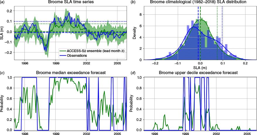
The ACCESS-S2 forecast for the probability P of exceeding the given quantile of the observed climatological SLA distribution is constructed based on the fraction of ensemble members that exceed the quantile (for the corresponding quantile level α) from the ACCESS-S2 climatological SLA distribution over the 1982–2018 hindcast period. Each quantile is computed separately for each lead time and tide gauge. The value of this quantile threshold may differ from the value of the quantile threshold from the observational distribution due to model biases (e.g. compare blue and green distributions in Fig. 2b). This method thus constitutes a bias correction. Example time series forecasts for the median and upper decile exceedance probabilities at Broome are shown in Fig. 2c, d.
Verification for these forecasts is based on the squared error in probability space, the Brier Score (BS):
where p is the ACCESS-S2 probability forecast and po is the binary event time series, equal to 1 if the observed SLA exceeds the quantile of the observed climatological SLA distribution and 0 otherwise (e.g. blue lines in Fig. 2c, d). The overline indicates an average over all start dates (either for a single month or for all months grouped together). As for the RMSE and CRPS, we compute a BS score (BSS) by comparing the ACCESS-S2 BS against BSref, the BS achieved by the best constant reference forecast probability, being the observed frequency of threshold exceedances over the hindcast period. Owing to the finite set of verification times, this observed frequency may differ somewhat from the theoretical expectation of pref = 1 − α. The ACCESS-S2 BS is also compared to a deterministic anomaly persistence forecast (i.e. whether the observed SLA for the month prior to the given start date exceeds the threshold).
Finally, to better understand the quantile exceedance skill, we perform a Consistent, Optimally binned, Reproducible, and Pool-Adjacent-Violators algorithm based (CORP) decomposition of the BSS (Dimitriadis et al. 2021; Loveday et al. 2024), which uses nonparametric isotonic regression to robustly decompose BS into miscalibration (MCB), discrimination (DSC) and uncertainty (BSref) terms:
Small values of MCB indicate that the forecast is reliable, in that the observed frequency of quantile exceedance for a given forecast probability matches that forecast probability. Larger values of DSC indicate that the forecast can discriminate between exceedance and non-exceedance. Using Eqn 5 allows us to express the BSS as follows:
where MCB/BSref = 0 indicates perfect reliability and DSC/BSref = 1 indicates perfect discrimination.
Note that the probabilistic (and deterministic) verification and computation of quantile threshold values is done here using all the data available. An alternative, which may be more appropriate for application to real-time forecasts, is to use a cross-validation approach where the skill is computed separately for each year (and then averaged across all years), with the data for the year being verified being dropped for the purpose of computing thresholds; also see McIntosh et al. (2015) for a discussion of the role of cross-validation under calibration. We tested this approach for the BSS skill metric and found only minor differences not exceeding 0.02 (relative to BSS values at skilful locations between 0.2 and 0.6) for the median and reaching ~0.1 (relative to 0.1–0.4) at a few isolated locations for upper tercile and upper decile exceedance. We thus chose not to use cross-calibration in our skill analyses.
For comparisons to altimetry (spatially resolved skill), the statistical significance of the ACC values is computed using an effective sample size of N(1 − ρfρo) ÷ (1 + ρfρo), where ρf and ρo are the lag-1 autocorrelations of the given forecast and observed time series of length N (~444 = 37 years × 12 months) respectively. For computing the significance of ACC differences, a Fisher-z transformation is applied following Shin and Newman (2021) and McIntosh et al. (2015). For all tide gauge computations, the Diebold–Mariano test (Diebold and Mariano 1995), with the Hering and Genton (2011) modification, on the time series of raw score differences at each time (e.g. the normalised anomaly product for ACC or the squared error for RMSE) is used to evaluate significance while taking into account autocorrelation with lead time. Following convention, we use P = 0.05 for significance.
3. Results
We begin with a brief analysis of the ACCESS-S2 ocean reanalysis from which the forecasts are initialised (Section 3.1) and assess ACCESS-S2’s representation of monthly SLA variance (Section 3.2). We then describe the spatial skill distribution for ACCESS-S2 ensemble mean sea level forecasts (including the IB) across all target calendar months (Section 3.3). This is followed by a detailed analysis of the skill at selected tide gauges as a function of target calendar month (Sections 3.4 and 3.5). The contribution of the IB to the forecast skill is considered in Section 3.6 and the skill of quantile exceedance probability forecasts is considered in Section 3.7.
3.1. Performance of the reanalysis
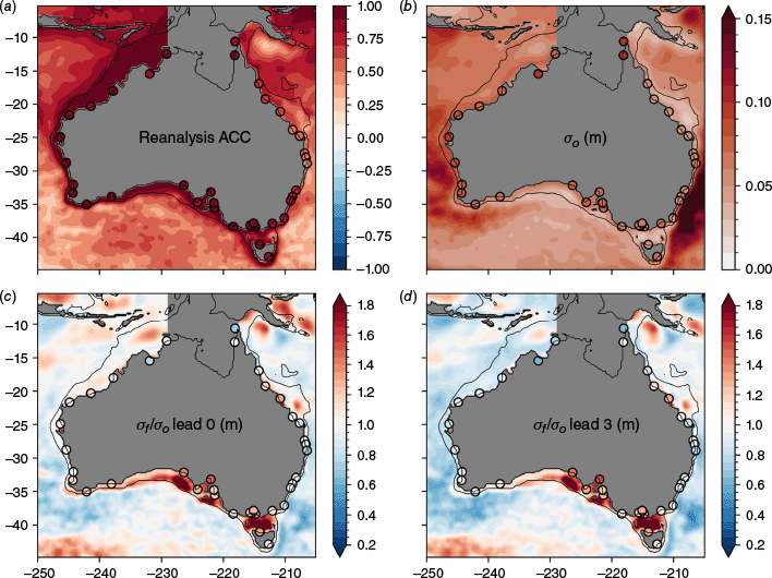
As discussed in more detail for the global context in Widlansky et al. (2023), the skill of ACCESS-S2 forecasts of seasonal sea level variability in the open ocean is lower than seasonal prediction systems whose reanalysis systems do assimilate altimetry observations. Focusing on the Australian region, Fig. 3a shows that the correlation between the ACCESS-S2 ocean reanalysis and satellite altimetry is relatively low in the open ocean. However, correlations are much higher at the coast, suggesting that the lack of assimilation of altimetry in the ACCESS-S2 reanalysis has little impact on the representation of coastal sea level variability. Here, assimilation of in situ temperature and salinity data, as well as satellite SST data, may contribute to directly constraining the sea level variability, in addition to teleconnections from other regions. It is important to note though that altimetry is not typically used inshore in most assimilation systems (Feng et al. 2024) as the signal-to-noise ratio is much smaller than in the open ocean. The correlation coefficients between the ACCESS-S2 ocean reanalysis and the ANCHORS tide gauges remain above 0.8 around most of the coast, with values only dropping below 0.8 for the east coast gauges between Sydney and Cairns (dots in Fig. 3a).
(a) Anomaly correlation coefficient (ACC) of linearly detrended monthly SLAs from the ACCESS-S2 ocean reanalysis compared to IMOS sea level and ANCHORS tide gauge observations over the 1993–2018 period. (b) The standard deviation of monthly SLAs from the observations. The standard deviation of monthly SLAs from the ACCESS-S2 hindcast ensemble members divided by the IMOS/ANCHORS observed standard deviation at lead month (c) 0 (corresponding to the first month of the forecast after initialisation, note that the magnitude of the variability in the reanalysis is similar to the lead 0 forecast, not shown) and (d) 3. Note that there are no data in the Gulf of Carpentaria in the IMOS dataset, which is depicted by grey shading.
3.2. Representation of sea level variance
Both the reanalysis and the hindcast also represent the overall amplitude of monthly SLAs (i.e. residual variability) along the coast well (Fig. 3c, noting that the reanalysis gives very similar results to the lead 0 forecast, not shown), though with some exceptions. Along the continental shelf edge in the Great Australian Bight and Bass Strait the variance appears to be overestimated by a factor of two. However, when instead compared to Copernicus satellite altimetry observations, the model variability is within 20% of the observations in this region. This suggests that this feature in Fig. 3c is largely an issue with the IMOS sea level product itself (note that the IMOS product compares much better with tide gauges around the coast than the Copernicus product, as expected, despite its poor performance along the continental shelf edge, not shown). When compared instead directly to the ANCHORS tide gauge data at the coast in these regions in the south and south-east, the modelled sea level variance is only overestimated by up to 50%. The variance in the open ocean is weakly underestimated by ACCESS-S2, which is likely due to the model’s coarse (1/4°) resolution that only partially resolves mesoscale eddies. Note also that the variance in the open ocean, and along the north-west and west coast, decreases somewhat at longer leads (compare Fig. 3c, d), suggesting that the assimilation of observational (in situ temperature and salinity) data somewhat enhances the sea level variance above what the model would naturally produce.
3.3. Ensemble mean forecast skill (all target months)
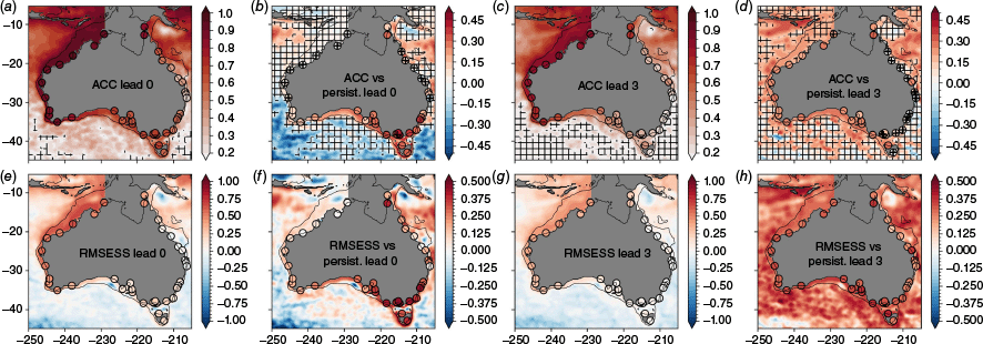
Consistent with past studies using the seasonal prediction system POAMA, the predecessor of ACCESS-S (Miles et al. 2014; McIntosh et al. 2015), the ACC skill of ACCESS-S2 is highest in the north-west and reduces anti-clockwise around the coast (Fig. 4a, c). The ACC on the east and south-east coasts decays rapidly beyond the first month, whereas in the west and north it remains above 0.7 out to lead month 3 (Fig. 5a, d). The ACC skill is statistically significant (i.e. better than a 0-anomaly forecast) around nearly the entire coastline, even out to lead month 3 (Fig. 4c). This is an improvement over POAMA (e.g. McIntosh et al. 2015), primarily as the longer ACCESS-S2 hindcast provides a larger sample size and improved statistics (e.g. lower ACCs can still be significant). At short lead times most of the skill on the west and north-west coasts comes from anomaly persistence. The ACC of the ACCESS-S2 forecast is not significantly better than an anomaly persistence forecast at most of these locations at lead 0, but does beat persistence as lead time increases (Fig. 4b, compare solid and dashed lines of Fig. 5a, d). Skill is significantly better than persistence along the south coast and particularly in the south-east at lead month 0 (Fig. 4b), highlighting the shorter decorrelation time scale of sea level variability in these regions. At longer leads (e.g. lead month 3, Fig. 4c, d) the model beats persistence on the west and much of the south coast, whereas on the east coast persistence and ACCESS-S2 forecasts have much lower, though still significant, ACC values.
Ensemble mean skill metrics for ACCESS-S2 sea level anomalies compared to satellite altimetry (continuous colour) and ANCHORS tide gauges (markers) over the 1993–2018 period. The anomaly correlation coefficient (ACC) at lead (a) 0 (corresponding to the first month of the forecast after initialisation) and (c) 3 months. (b, d) The ACCESS-S2 ACC minus the ACC of an anomaly persistence forecast. Hatching indicates values that are (a, c) not significant, or (b, d) not significantly better than an anomaly persistence, at P = 0.05. The RMSE Skill Score (RMSESS) at lead (e) 0 and (g) 3 months. A value of 0 or less indicates no skill compared to a 0-anomaly forecast, with a value of 1 being perfect (zero RMSE). (f) The ACCESS-S2 RMSESS minus the RMSESS of an anomaly persistence forecast compared to altimetry and tide gauges. (h) The ratio of the standard deviation of individual ensemble members of the ACCESS-S2 forecast (averaged across ensemble members) at lead 0 months to the observations. All metrics are for all target calendar months together. Note that there are no data in the Gulf of Carpentaria in the IMOS dataset, which is depicted by grey shading.
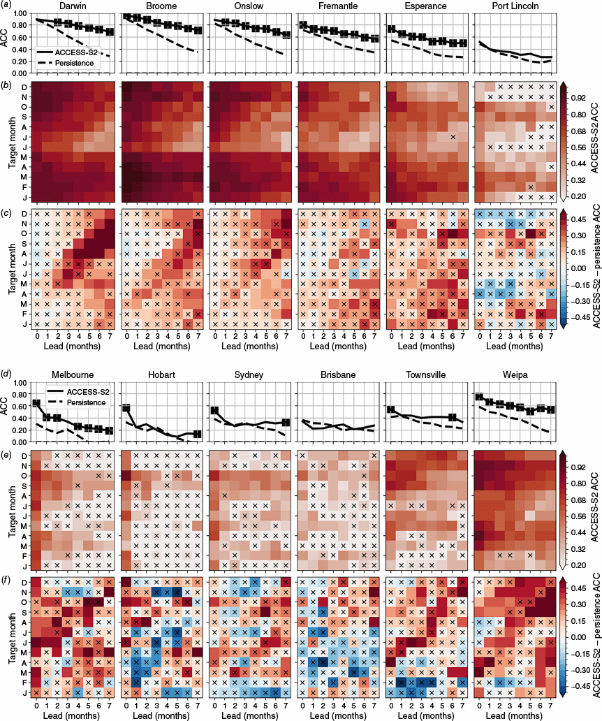
ACC skill at selected ANCHORS tide gauges. (a, d) ACC from ACCESS-S2 (solid line) and for persistence (dashed line) across all target calendar months as a function of lead month for the period 1982–2018. Solid squares mark values where the ACCESS-S2 ACC is significantly better than persistence at P = 0.05 according to the Diebold–Mariano test. (b, e) ACC from ACCESS-S2 as a function of lead and target calendar month. (c, f) ACC difference between ACCESS-S2 and an anomaly persistence forecast. Crosses mark values that are not significant (b, e) or not significantly better than persistence (c, f) at P = 0.05 according to the Diebold–Mariano test. See Fig. 1 for tide gauge locations.
The RMSESS illustrates similar spatial and temporal patterns as ACC (Fig. 4e–g). However, at longer leads the ACCESS-S2 RMSE is much better than persistence (Fig. 4h). This is because the variance of the ACCESS-S2 ensemble mean forecast reduces with lead (an appropriate representation of forecast uncertainty) whereas the variance of an anomaly persistence forecast remains constant with lead (an overconfident forecast).
3.4. Ensemble mean forecast skill (individual target months)
Although Fig. 4 gives a good overview of the spatial structure of model skill, it does not indicate how skill may vary seasonally. Here, these variations are explored at key tide gauges.
The ACC skill for ACCESS-S2 is significantly better than 0 for all monthly leads and all target calendar months on the north-west and west coasts (Fig. 5b). At longer leads, forecast skill here is reduced for winter target months. This is likely associated with the ENSO spring predictability barrier (Latif et al. 1998), although increased stochastic variability in winter may also affect locations along the south-west coast. Most of this skill is again associated with persistence. The ACC of the ACCESS-S2 forecast is not significantly better than an anomaly persistence forecast for most leads and most months on the north-west and west coasts (Fig. 5c). The exception is at longer leads in Darwin in northern Australia in the second half of the year, which likely reflects the fact that changes in ENSO phase – which ACCESS-S2 can capture but anomaly persistence cannot – typically occur in the middle of the year. On the south and east coasts, ACC decreases rapidly with lead time and is not significant at most lead times beyond lead month 0 for Melbourne, Hobart, Sydney and Brisbane, apart from for a few specific target months (e.g. August–October in Melbourne). This lack of statistical significance differs from the case when all target months are grouped together (Fig. 4 and 5a), due to the factor of 12 smaller sample size. On the north-east coast skill is restored, e.g. for Townsville and Weipa particularly in the second half of the year (see Section 4 for a discussion of the causes behind these skill variations).
Generally, the RMSESS is less significant, compared to a reference forecast of 0 anomaly, than the ACC (see Supplementary Fig. S2). However, the ACCESS-S2 RMSE generally beats anomaly persistence more often than for the ACC because the RMSE metric naturally takes into account the reduction in the ensemble mean variance, and thus increase in forecast uncertainty, with lead time (unlike the ACC, which is computed from normalised time series).
3.5. Ensemble forecast skill
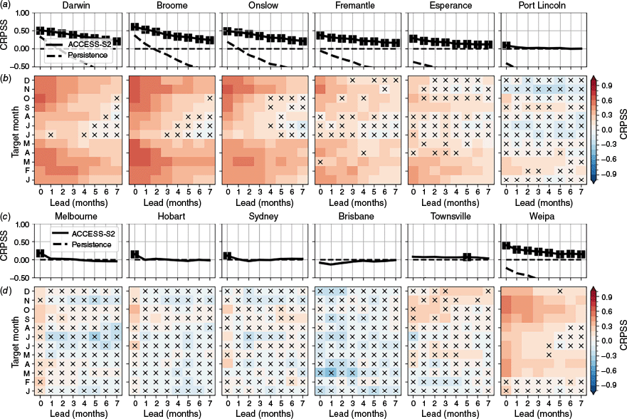
To take ensemble information into account (the ACC and RMSESS metrics consider only the ensemble mean forecast), we now analyse the CRPS and CRPSS metrics (Fig. 6, see Methods). ACCESS-S2’s CRPS is significantly better than a climatological reference forecast for most months on the north-west and west coasts, except for long leads in winter. Conversely, across the south and east coasts, CRPS is not significantly better than climatology for most leads and most months, although there is still some positive values at shorter lead times. Unlike the ACC, ACCESS-S2’s CRPSS is significantly better than anomaly persistence at the majority of leads and target months (compare solid and dashed lines in top row, and lack of red crosses in bottom row, of Fig. 6). For forecast use cases that properly utilise uncertainty information available in ACCESS-S2’s ensemble, the CRPSS is the appropriate skill score to base skill assessment on (rather than the ACC or RMSESS).
As for Fig. 5 but for the CRPS skill score CRPSS (see Methods). Values above 0 indicate skill compared to a climatological reference forecast (e.g. forecasting the climatological distribution of sea level), with a maximum value of 1 (corresponding to a perfect, certain forecast). Squares (a and c) indicate CRPS scores that are significantly better than both the climatological reference forecast (i.e. CRPSS is significantly greater than 0) and anomaly persistence (dashed line) according to the Diebold–Mariano test at P = 0.05. Black (red) crosses (b and d) indicate CRPS scores that are not significantly better than the climatological reference forecast (anomaly persistence forecast) according to the Diebold–Mariano test at P = 0.05.
3.6. Role of inverse barometer
We now consider the skill of forecasts of the IB, derived from ACCESS-S2’s sea level pressure forecast as a post-processing step, and whether including the IB affects the total sea level forecast skill.
As discussed in the Introduction, the standard deviation of the monthly averaged IB is highest in the mid-latitudes and reaches an amplitude of ~±4 cm (Fig. 7d) that is 10–20% of the total sea level variance (orange line in Fig. 1c). The spatial scales of the IB are large and so here we summarise skill at four representative tide gauges (Fig. 7). The ACC and RMSESS for ACCESS-S2’s IB forecasts are both highest in the north and lowest in the south. This is consistent with the larger role for chaotic, weather-driven variability in the mid-latitudes and the predominance of predictable, tropical climate mode-driven variability in the north. When computed across all target calendar months (Fig. 7a, b, e), the ACC is significant at all sites and leads. It remains above 0.4 in the north and south-west but reduces to 0.2 in the south-east beyond lead month 4. As a function of target month (Fig. 7g), ACC is significant in the north except at longer leads in winter. The ACC is a little lower in the south-west and considerably lower in the south-east, where the ACC is barely significant beyond the first month.
ACC, RMSESS and CRPSS of the ACCESS-S2 IB forecast compared to ERA-5 over the 1982–2018 period. ACC skill at lead (a) 0 and (b) 3 months. Values that are not significant are hatched. (c) RMSESS at lead 3 months. (d) The standard deviation of the observed IB (m). (e) ACC and (f) CRPSS for all target months together at selected tide gauge locations. (g) ACC and (h) CRPSS as a function of target calendar month. Squares (e and f) note significant skill, whereas black crosses (g and h) indicate skill that is not significantly better than a reference forecast of 0 anomaly at P = 0.05 according to the Diebold–Mariano test.
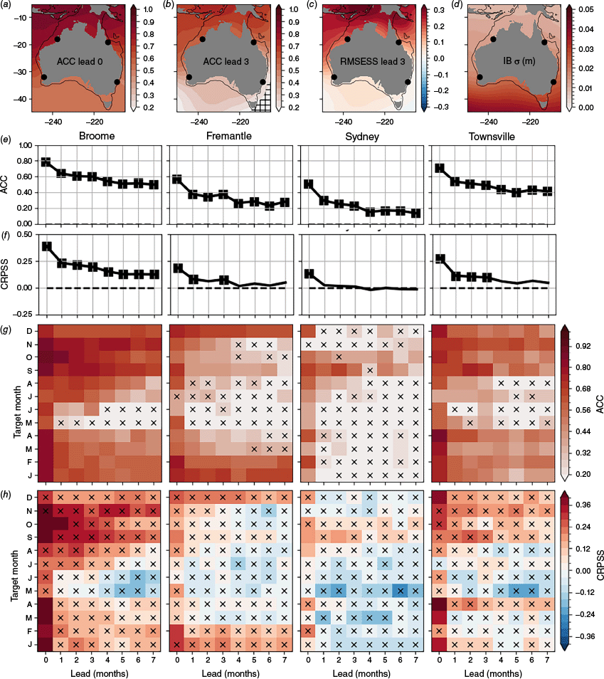
The spatial structure of the CRPSS (Fig. 7f, h) is similar to the ACC, and indicates that ACCESS-S2 is better than a reference climatology forecast in similar regions and times of year (indicated by red in Fig. 7h). However, as a function of target calendar month, the CRPSS is non-significant nearly everywhere. This is because, unlike the ACC that only considers the ensemble mean, the CRPSS takes into account the ensemble variability that is (compared to the ensemble mean) relatively large for the IB, due to the stochasticity of atmospheric variability.
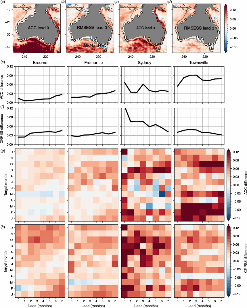
Despite the fact that the forecast of the IB alone is not skilful everywhere, including IB in the ACCESS-S2 forecast improves the ACC, RMSESS and CRPSS sea level forecast skills in nearly all cases (Fig. 8). This is because including the IB leads to a better representation of the overall sea level variance and forecast uncertainty. The degree of improvement varies with location and lead time, depending on the skill of the IB forecast alone, skill of the dynamic sea level forecast and the fraction of variability accounted for by the IB. Improvements are largest on the east coast with ACC, RMSESS and CRPSS improvements reaching ~0.1.
Difference in skill when including the IB in the ACCESS-S2 forecast, compared to observations of the total sea level including the IB. ACC difference at lead (a) 0 and (b) 3 months over the 1993–2018 period. RMSESS difference at lead (c) 0 and (d) 3 months over the 1993–2018 period. (e, g) ACC and (f, h) CRPSS difference as a function of lead for (e, f) all target calendar months together and (g, h) as a function of target calendar month at selected tide gauges over the 1982–2018 period. (a–d) Note that there are no data in the Gulf of Carpentaria in the IMOS dataset, which is depicted by grey shading.
3.7. Quantile exceedance probability skill
Forecast users are often interested in the probability of exceeding various thresholds, for use in risk assessments. In this section, we perform a skill analysis for ACCESS-S2 forecasts of the probability of exceeding the median, upper tercile and upper deciles of the observed climatological SLA distribution. The construction of these forecasts is described in the Methods and an example is shown in Fig. 2. Here, the BS and BSS are used to quantify the skill of these forecasts (see Methods).
As for the total sea level forecast, the skill of the quantile exceedance forecasts is highest on the north and west coasts and reduces anti-clockwise around the coast (Fig. 9a, d, e), with a distinct drop in forecast skill at leads more than 1 month across the Great Australian Bight east of the Esperance tide gauge (consistent with similar drops in ACC and RMSESS, Fig. 4c, g). The BSS for median and upper tercile exceedance is significantly better than a constant reference forecast on the north and west coasts at all leads, reaching values ~0.6 out of a maximum of 1. For upper decile exceedance the significance of the skill is reduced at long leads compared to the median and upper tercile due to the reduced number of observed events. On the south and south-east coasts, the BSS for median exceedance is significant at leads of 0–3 months and for upper tercile exceedance at leads of 0–1 months, but there is little skill on the east coast. ACCESS-S2 has more accurate probability predictions than overly confident (i.e. no uncertainty) anomaly persistence forecasts (lack of white crosses in Fig. 9a, d, e).
The Brier Skill Score (see Methods) for ACCESS-S2 probability forecasts for exceedance of the (a) median α = 0.5, (d) upper tercile α = 2/3 and (e) upper decile α = 9/10 over the 1982–2018 period. 0 indicates no skill improvement over the constant reference forecast (the observed frequency of events) whereas 1 indicates a perfect score. Values that are not better than the constant reference forecast (anomaly persistence) at P = 0.05 according to the Diebold–Mariano test are indicated with a black (white) cross (note that these two sets of crosses are offset). The (b) miscalibration MCB and (c) discrimination DSC components of the BSS from the CORP decomposition (Eqn 6) for the median exceedance forecast. Values of MCB/BSref near zero indicate a well calibrated (or reliable) forecast whereas larger values of DSC/BSref indicate that the forecast can better discriminate between observed exceedances and non-exceedances.
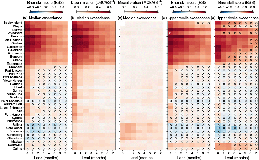
At tide gauge locations with positive BSS values, the reliability of the forecast probabilities is very good (MCB is near 0, Fig. 9c). Consequently, the locations with the best BSS scores are those where the forecasts are best able to discriminate between events, as quantified by the CORP discrimination score (DSC, Fig. 9b). Note that DSC gives similar information to the area under the Relative Operating Characteristic curve (not shown). Example reliability diagrams illustrate these results in more detail (Supplementary Fig. S3), with reliability curves remaining within the uncertainty bounds around the 1-to-1 line at all locations except along the east coast (e.g. Brisbane, Supplementary Fig. S3f).
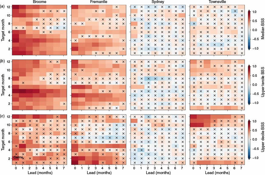
The results in Fig. 9 are computed across all target calendar months (with quantile thresholds computed using data from all months) and thus benefit from a large sample size. When considered as a function of target calendar month (with quantile thresholds computed individually for each month), the significance of the BSS values is reduced. However, the spatial pattern is similar to that for all months. Example BSS values as a function of target and lead month are shown in Fig. 10 for the Broome, Fremantle, Sydney and Townsville tide gauges. Note that the colour bar in Fig. 10 ranges between −1 and 1, rather than −0.6 and 0.6 in Fig. 9, as the BSS can be higher for specific months.
Brier Skill Score for ACCESS-S2 probability forecasts for exceedance of the (a) median α = 0.5, (b) upper tercile α = 2/3 and (c) upper decile α = 9/10 over the 1982–2018 period at the Broome, Fremantle, Sydney and Townsville tide gauges as a function of lead month and target calendar month. 0 indicates no skill improvement over the constant reference forecast (the observed frequency of events) whereas 1 indicates a perfect score. Values that are not significantly better than the constant reference forecast (anomaly persistence) at P = 0.05 according to the Diebold–Mariano test are indicated with a black (white) cross. Note that unlike in Fig. 9, here the quantile thresholds are computed individually for each target calendar month.
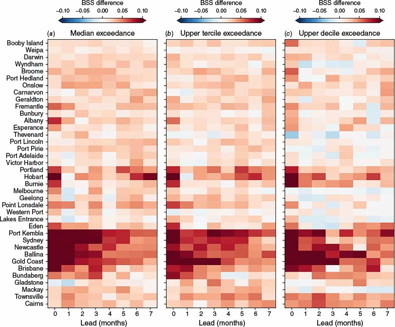
Finally, we note that inclusion of the IB improves the skill of the quantile exceedance forecasts, with BSS increases of order 0.05 around most of the coastline, increasing to more than 0.1 at leads of 0–3 months on the east coast (Fig. 11).
The difference in the Brier Skill Score (see methods) for ACCESS-S2 probability forecasts for exceedance of the (a) median q = 0.5, (b) upper tercile q = 2/3 and (c) upper decile q = 9/10 over the 1982–2018 period when including the IB component in the forecast (compared to exceedances of quantiles of observed total sea level anomalies including the IB in both cases). All target calendar months are considered together.
4.Mechanisms for predictability
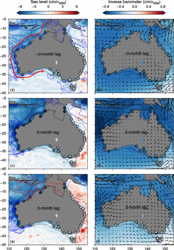
As shown by Miles et al. (2014) and McIntosh et al. (2015), the major source for predictability of Australian coastal sea level at seasonal time scales is ENSO, which drives up to 60% of the monthly sea level variance on the north and west coasts (green line in Fig. 1c, also see White et al. 2014). ACCESS-S2 has skill in forecasting ENSO beyond 6 months of lead time compared to reference forecasts (Wedd et al. 2022, e.g. their fig. 4). The peak correlation between ENSO and Australian coastal sea level occurs at a relatively short lag of no more than ~1 month (not shown). This is consistent with an oceanic teleconnection propagated by CTW dynamics from the Western Pacific and Maritime Continent with the coast on their left (Fig. 12a, c, e, Miles et al. 2014; McIntosh et al. 2015), travelling at wave speeds near the first-baroclinic Kelvin wave speed in the tropics of ~3 m s−1 (Chelton et al. 1998), which subsequently affect the shelf sea level through changes in coastal currents, mass and density (temperature and salinity). Other mechanisms that could explain the connection between ENSO and Australian coastal sea level include local air-sea fluxes and wind-driven Ekman transport (Roberts et al. 2016). The SSTs are generally cooler on the west and north-west coasts during El Niño events (blue contours in Fig. 12a, c, e), which drive positive (into the ocean) air–sea heat flux anomalies (confirmed through analysis of air–sea flux observations from OAFlux, see https://oaflux.whoi.edu/, not shown) of the wrong sign to contribute to the negative SLAs by locally driven thermosteric contraction. Wind anomalies during El Niño events do have an upwelling-favourable south-westerly component on the north-west shelf that may contribute to driving low SLAs (vectors in Fig. 12b, d, f). The Great Barrier Reef region also shows some evidence of weak northerly, upwelling favourable winds correlated with low coastal sea level, but elsewhere local wind-driven mechanisms at this time scale are not supported by the regression analysis. Therefore, the main mechanism is likely associated directly with CTWs and their impacts on currents, vertically integrated mass and density – Jacox et al. (2023) came to a similar conclusion for the California current.
Lag regressions of monthly mean sea level anomalies (a, c, e, including the IB) and the IB (b, d, f) onto the Niño 3.4 index at (a, b) −3, (c, d) 0 and (e, f) 3 months lag in the units of centimetres per standard deviation of the Niño 3.4 index (σN34) over the 1993–2018 period. Negative lags indicate the Niño 3.4 index leading. Contours (a, c and e) indicate lag regressions of SST anomalies (from NOAA’s OISST product over 1993–2018) onto the Niño 3.4 index, with red contours indicating positive values above 0.1°C/σN34 and blue contours indicating negative values below −0.1°C/σN34, with a contour level of 0.05°/σN34. (a, c and e) Note that there are no data in the Gulf of Carpentaria in the IMOS dataset, which is depicted by grey shading. Vectors (b, d and f) indicate lag regressions of wind anomalies (from ERA5 over 1993–2018) onto the Niño 3.4 index. The red arrow (a) indicates the pathway for coastal trapped waves propagating from the western equatorial Pacific Ocean.
There is a distinct reduction in most seasonal skill metrics across the Great Australian Bight (beyond the Esperance tide gauge, e.g. see Fig. 9), which may be associated with the widening of the shelf, increased dissipation of seasonal signals and an increased role for stochastic, high-frequency weather-driven variability, e.g. Woodham et al. (2013) showed that high-frequency CTW amplitudes increase in amplitude in this region. On the south-east, east and north-east coasts of Australia, the connection between ENSO and the local sea level is much weaker (Fig. 12a, c, e), resulting in a small monthly averaged sea level variance (Fig. 1c) and a lack of predictability (Fig. 4).
However, ENSO’s atmospheric teleconnections do have a local impact through the IB effect, reaching almost 1 cm per standard deviation of the Niño 3.4 index (Fig. 12b, d, f), and, possibly, through local wind-driven effects as discussed above. Although the strength of the IB connection to ENSO is relatively uniform around the coast, the biggest impact of IB on the skill of the total sea level forecast is on the east coast (Fig. 8, 11) because the relative strength of the IB (compared to the total sea level variance) is strongest here (orange line in Fig. 1c). The higher relative strength of the IB also explains why the skill on the north-east shelf (e.g. at Townsville, see Fig. 5) is highest in austral spring and early summer, when the atmospheric ENSO teleconnections to this region are strongest (e.g. Risbey et al. 2009). Note the distinct difference between the behaviour of the shelf and the open ocean here (Fig. 12a, c, e, Woodworth et al. 2019), with El Niño driving significant positive SSH anomalies off the shelf through thermosteric expansion associated with clear skies, atmospheric heating and warm SSTs, in contrast to the negative anomalies near the coast.
In Section 3.3 it was found that there was some skill compared to reference forecasts in the south-east at certain times of year beyond lead month 1 (e.g. August–October in Melbourne and Sydney, Fig. 5). The seasonal relationship between ENSO and south-eastern sea level is strongest around this time of year (see Supplementary Fig. S4), suggesting that this skill is likely due to ENSO teleconnections.
Other potential sources for seasonal predictability include the IOD, the SAM and the Madden–Julian Oscillation (MJO). Regression analysis suggests that the IOD does not drive much sea level variability along the Australian coastline, when isolated from its impact on ENSO (not shown, also see Frankcombe et al. 2015). However, note that the IOD does affect Australian coastal sea level through the IB (reaching ~1 cm, see fig. 2 of Roberts et al. 2016). The SAM explains up to 15% of the variance of sea level along the south coast (red line in Fig. 1c). However, beyond a month of lead time, the predictability of the SAM is limited and thought to be due to its connection to ENSO (Lim et al. 2013). The MJO has a strong influence on coastal sea level in the Gulf of Carpentaria at short lead times (e.g. Oliver and Thompson 2010), but weak elsewhere. A more detailed analysis of sea level forecast skill associated with the MJO will be undertaken in a subsequent study on subseasonal forecast skill. Given the weak connection of these other modes of variability to Australian coastal sea level, we conclude, in agreement with previous studies (Miles et al. 2014; McIntosh et al. 2015) that ENSO is the dominant source of predictability.
5.Summary and next steps
We have quantified the skill of the seasonal ensemble prediction system, ACCESS-S2, in forecasting monthly SLAs (from the mean climatology) around the Australian coast up to 8 months into the future as compared to satellite altimetry and tide gauge observations and various reference forecasts.
We showed that including the IB effect in the monthly SLA forecasts, as a post-processing step using ACCESS-S2’s atmospheric sea level pressure forecasts, improves skill at the majority of coastal locations (Fig. 8). Seasonal SLA forecast skill can be improved by adding the IB, even if the skill of the IB forecast alone is not significantly better than a reference forecast, due to an improved representation of the overall sea level variability and uncertainty. This improvement is particularly notable on the east coast, where the IB contributes a larger fraction of the total sea level variability.
Seasonal sea level forecast skill is highest on the north and west coasts, where oceanic teleconnections with ENSO by CTWs and their impacts on shelf currents, mass and density, are strongest (Section 4, also see Miles et al. 2014; White et al. 2014; McIntosh et al. 2015), and reduces anti-clockwise around the coast (Fig. 5). Atmospheric ENSO teleconnections also contribute some skill by the IB effect and wind-driven Ekman processes (Section 4), whereas other modes of variability and processes contribute minimal skill. Because ENSO is a relatively long-lived phenomenon, much of the skill of the ensemble mean SLA forecast is due to anomaly persistence. However, skill metrics that take into account the uncertainty information available in the ACCESS-S2 ensemble, such as the CRPS (Fig. 6) or the BSS for quantile exceedance probability forecasts (BSS; Fig. 9), do show significant improvement over reference forecasts at most leads on the north and west coasts, and at shorter leads on the south coast.
Real time ACCESS-S2 forecasts of seasonal SLAs (without the IB) are currently produced for the Pacific through the Climate and Oceans Support Program in the Pacific (COSPPac; see http://www.bom.gov.au/climate/pacific/outlooks/), and also provided to the Australian Defence Force by regular briefings. These basic offerings will be leveraged by the Australian Climate Service to develop more sophisticated products for the Australian coastal zone. A prototype seasonal high-water alert product suite for the Australian coastline, building on the approach of Dusek et al. (2022), is under development, incorporating real time ACCESS-S2 sea level forecasts, tide predictions and sea level rise estimates. The seasonal SLA forecast component of this system will be most useful along the north-west and west Australian coasts, where the predictable seasonal anomalies reach up to 50% of the total sea level variance (e.g. Fig. 1c). Note that the benefits and practicality of including sea level trends into such a product suite, as discussed in Section 2.3.3, still need to be determined. The potential benefit of coastal downscaling (e.g. Long et al. 2023; Jacox et al. 2023) and calibration approaches – such as the quantile–quantile matching used for ACCESS-S2 terrestrial forecasts, National Operations Centre (2019), also see McIntosh et al. (2015) – will also be explored during product development. Future work will also assess model sea level skill on subseasonal (1–6 weeks) time scales, with recent studies suggesting that there may be some potential at this time scale (e.g. Amaya et al. 2022) associated with Kelvin waves that have a peak period of 10–25 days around the Australian coastline (Woodham et al. 2013), and with the MJO in the Gulf of Carpentaria (Oliver and Thompson 2010). In the longer term, an operational service incorporating this new prototype product suite is planned to better inform decision making and increase Australian community resilience to coastal flooding hazards under climate change.
Data availability
ACCESS-S2 hindcast and reanalysis data are available at https://doi.org/10.25914/60627ad0ba3ee and https://doi.org/10.25914/60627ad8878e2. ANCHORS tide gauge data are available at https://doi.org/10.25914/6142dff37250b. Satellite altimetry data were sourced from Australia’s Integrated Marine Observing System (IMOS) – IMOS is enabled by the National Collaborative Research Infrastructure Strategy. Dynamic atmospheric corrections are produced by CLS using the Mog2D model from Legos and distributed by AVISO+, with support from CNES (see https://www.aviso.altimetry.fr/). This study has been conducted using EU Copernicus Marine Service Information and Marine Data Store (2022).
Conflicts of interest
The authors declare that the research was conducted in the absence of any commercial or financial relationships that could be construed as a potential conflict of interest.
Declaration of funding
This research has been funded by the Australian Climate Service. The Australian Climate Service is a partnership made of the Bureau of Meteorology, CSIRO, the Australian Bureau of Statistics and Geosciences Australia. The authors acknowledge the use of the National Computational Infrastructure that is supported by the Australian Government.
Acknowledgements
We thank the Bureau of Meteorology seasonal prediction teams for their work developing and maintaining ACCESS-S2. We acknowledge the developers of the forecast verification Python packages climpred (see https://github.com/pangeo-data/climpred), scores (see https://github.com/nci/scores) and xskillscore (see https://xskillscore.readthedocs.io/en/stable/index.html). We thank Rob Taggart for assistance with verification metrics and reviewers Ben Hague and Xiaobing Zhou (Bureau of Meteorology) for their early reviews and feedback.
Author contributions
R. Holmes performed the analyses and wrote the initial draft. All authors contributed to the generation of ideas and drafting of the final manuscript.
References
Abhik S, Hope P, Hendon HH, Hutley LB, Johnson S, Drosdowsky W, et al. (2021) Influence of the 2015–2016 El Niño on the record-breaking mangrove dieback along northern Australia coast. Scientific Reports 11, 20411.
| Crossref | Google Scholar | PubMed |
Amaya DJ, Jacox MG, Dias J, Alexander MA, Karnauskas KB, Scott JD, et al. (2022) Subseasonal-to-seasonal forecast skill in the california current system and its connection to coastal Kelvin waves. Journal of Geophysical Research: Oceans 127, e2021JC017892.
| Crossref | Google Scholar |
Ampou EE, Johan O, Menkes CE, Niño F, Birol F, Ouillon S, et al. (2017) Coral mortality induced by the 2015–2016 El Niño in Indonesia: the effect of rapid sea level fall. Biogeosciences 14, 817-826.
| Crossref | Google Scholar |
Archiving, Validation and Interpretation of Satellite Oceanographic (2023) Dynamic atmospheric corrections are produced by CLS using the Mog2D model from Legos and distributed by Aviso+, with support from CNES. (AVISO) [Dataset] doi:10.24400/527896/a01-2022.001
Barroso A, Wahl T, Li S, Enriquez A, Morim J, Dangendorf S, et al. (2024) Observed spatiotemporal variability in the annual sea level cycle along the global coast. Journal of Geophysical Research: Oceans 129, e2023JC020300.
| Crossref | Google Scholar |
Brown BE, Dunne RP, Somerfield PJ, Edwards AJ, Simons WJF, Phongsuwan N, et al. (2019) Long-term impacts of rising sea temperature and sea level on shallow water coral communities over a 40 year period. Scientific Reports 9, 8826.
| Crossref | Google Scholar | PubMed |
Chelton DB, deSzoeke RA, Schlax MG, El Naggar K, Siwertz N (1998) Geographical variability of the first baroclinic Rossby radius of deformation. Journal of Physical Oceanography 28, 433-460.
| Crossref | Google Scholar |
Cooley S, Schoeman D, Bopp L, Boyd P, Donner S, Ghebrehiwet D, et al. (2022) 3 – Oceans and Coastal Ecosystems and Their Services. In ‘Climate Change 2022 – Impacts, Adaptation and Vulnerability: Working Group II Contribution to the Sixth Assessment Report of the Intergovernmental Panel on Climate Change’. pp. 379–550. (Cambridge University Press) 10.1017/9781009325844.005
Diebold FX, Mariano RS (1995) Comparing predictive accuracy. Journal of Business and Economic Statistics 13, 253-263.
| Crossref | Google Scholar |
Dimitriadis T, Gneiting T, Jordan AI (2021) Stable reliability diagrams for probabilistic classifiers. Proceedings of the National Academy of Sciences of the United States of America 118, e2016191118.
| Crossref | Google Scholar | PubMed |
Dusek G, Sweet WV, Widlansky MJ, Thompson PR, Marra JJ (2022) A novel statistical approach to predict seasonal high tide flooding. Frontiers in Marine Science 9, 1073792.
| Crossref | Google Scholar |
EU Copernicus Marine Service Information Marine Data Store (2022) Global ocean gridded L4 sea surface heights and derived variables reprocessed 1993 ongoing. (CMEMS and MDS) 10.48670/moi-00148
Feng X, Widlansky MJ, Balmaseda MA, Zuo H, Spillman CM, Smith G, et al. (2024) Improved capabilities of global ocean reanalyses for analysing sea level variability near the Atlantic and Gulf of Mexico Coastal US. Frontiers in Marine Science 11, 1338626.
| Crossref | Google Scholar |
Fogt RL, Marshall GJ (2020) The Southern Annular Mode: variability, trends, and climate impacts across the Southern Hemisphere. WIREs Climate Change 11, e652.
| Crossref | Google Scholar |
Frankcombe LM, McGregor S, England MH (2015) Robustness of the modes of Indo-Pacific sea level variability. Climate Dynamics 45, 1281-1298.
| Crossref | Google Scholar |
Gregory JM, Griffies SM, Hughes CW, Lowe JA, Church JA, Fukimori I, et al. (2019) Concepts and terminology for sea level: mean, variability and change, both local and global. Surveys in Geophysics 40, 1251-1289.
| Crossref | Google Scholar |
Hague BS, Jones DA, Trewin B, Jakob D, Murphy BF, Martin DJ, et al. (2022) ANCHORS: a multi-decadal tide gauge dataset to monitor Australian relative sea level changes. Geoscience Data Journal 9, 256-272.
| Crossref | Google Scholar |
Hering AS, Genton MG (2011) Comparing spatial predictions. Technometrics 53, 414-425.
| Crossref | Google Scholar |
Hersbach H, Bell B, Berrisford P, Hirahara S, Horányi A, Muñoz-Sabater J, et al. (2020) The ERA5 global reanalysis. Quarterly Journal of the Royal Meteorological Society 146, 1999-2049.
| Crossref | Google Scholar |
Hudson D, Alves O, Hendon HH, Lim E-P, Liu G, Luo J-J, et al. (2017) ACCESS-S1: the new Bureau of Meteorology multi-week to seasonal prediction system. Journal of Southern Hemisphere Earth Systems Science 67, 132-159.
| Crossref | Google Scholar |
Integrated Marine Observing System (2023) IMOS 2023, oceancurrent – gridded sea level anomaly – delayed mode – dm02. (IMOS) Available at https://catalogue-imos.aodn.org.au/geonetwork/srv/eng/catalog.search#/metadata/da30c0b8-4978-4a26-915e-b80c88bb4510
Jacox MG, Buil MP, Brodie S, Alexander MA, Amaya DJ, Bograd SJ, et al. (2023) Downscaled seasonal forecasts for the California current system: skill assessment and prospects for living marine resource applications. PLoS Climate 2, e0000245.
| Crossref | Google Scholar |
Latif M, Anderson D, Barnett T, Cane M, Kleeman R, Leetmaa A, et al. (1998) A review of the predictability and prediction of ENSO. Journal of Geophysical Research 103, 14375-14393.
| Crossref | Google Scholar |
Lim E-P, Hendon HH, Rashid H (2013) Seasonal predictability of the Southern Annular Mode due to Its association with ENSO. Journal of Climate 26, 8037-8054.
| Crossref | Google Scholar |
Long X, Widlansky MJ, Spillman CM, Kumar A, Balmaseda M, Thompson PR, et al. (2021) Seasonal forecasting skill of sea-level anomalies in a multi-model prediction framework. Journal of Geophysical Research: Oceans 126, E2020JC017060.
| Crossref | Google Scholar |
Long X, Shin S-I, Newman M (2023) Statistical downscaling of seasonal forecasts of sea level anomalies for US coasts. Geophysical Research Letters 50, e2022GL100271.
| Crossref | Google Scholar |
Loveday N, Taggart R, Khanarmuei M (2024) A user-focused approach to evaluating probabilistic and categorical forecasts. Weather and Forecasting 39, 1163-1180.
| Crossref | Google Scholar |
Lowe RJ, Cuttler MVW, Hansen JE (2021) Climatic drivers of extreme sea level events along the coastline of Western Australia. Earth’s Future 9, e2020EF001620.
| Crossref | Google Scholar |
Madec G, Bourdallé-Badie R, Bouttier P-A, Bricard C, Bruciaferri D, Calvert D (2013) NEMO ocean engine. Note du Pôle de modélisation de l’Institut Pierre-Simon Laplace, Number 27. Zenodo 2013, ver. 3.4-patch [Software documentation, published 11 February 2013].
| Crossref | Google Scholar |
Marshall GJ (2003) Trends in the Southern Annular Mode from observations and reanalyses. Journal of Climate 16, 4134-4143.
| Crossref | Google Scholar |
McIntosh PC, Church JA, Miles ER, Ridgway K, Spillman CM (2015) Seasonal coastal sea level prediction using a dynamical model. Geophysical Research Letters 42, 6747-6753.
| Crossref | Google Scholar |
Megann A, Storkey D, Aksenov Y, Alderson S, Calvert D, Graham T, et al. (2014) GO5.0: the joint NERC–Met Office NEMO global ocean model for use in coupled and forced applications. Geoscientific Model Development 7, 1069-1092.
| Crossref | Google Scholar |
Middleton JF, Arthur C, Ruth PV, Ward TM, McClean JL, Maltrud ME, et al. (2007) El Niño effects and upwelling off South Australia. Journal of Physical Oceanography 37, 2458-2477.
| Crossref | Google Scholar |
Miles ER, Spillman CM, Church JA, McIntosh PC (2014) Seasonal prediction of global sea level anomalies using an ocean–atmosphere dynamical model. Climate Dynamics 43, 2131-2145.
| Crossref | Google Scholar |
Moftakhari HR, AghaKouchak A, Sanders BF, Matthew RA (2017) Cumulative hazard: the case of nuisance flooding. Earth’s Future 5, 214-223.
| Crossref | Google Scholar |
Mortensen E, Tiggeloven T, Haer T, van Bemmel B, Le Bars D, Muis S, et al. (2024) The potential of global coastal flood risk reduction using various DRR measures. Natural Hazards and Earth System Sciences 24, 1381-1400.
| Crossref | Google Scholar |
National Operations Centre (2019) Operations Bulletin Number 124. Operational Implementation of ACCESS-S1 Forecast Post-Processing. 16 September 2019. (Bureau of Meteorology, Commonwealth of Australia) Available at http://www.bom.gov.au/australia/charts/bulletins/opsull-124-ext.pdf
Oliver ECJ, Thompson KR (2010) Madden–Julian Oscillation and sea level: local and remote forcing. Journal of Geophysical Research: Oceans 115, C01003.
| Crossref | Google Scholar |
Ponte RM (1994) Understanding the relation between wind- and pressure-driven sea level variability. Journal of Geophysical Research: Oceans 99, 8033-8039.
| Crossref | Google Scholar |
Risbey JS, Pook MJ, McIntosh PC, Wheeler MC, Hendon HH (2009) On the remote drivers of rainfall variability in Australia. Monthly Weather Review 137, 3233-3253.
| Crossref | Google Scholar |
Roberts CD, Calvert D, Dunstone N, Hermanson L, Palmer MD, Smith D (2016) On the drivers and predictability of seasonal-to-interannual variations in regional sea level. Journal of Climate 29, 7565-7585.
| Crossref | Google Scholar |
Shin S-I, Newman M (2021) Seasonal predictability of global and North American coastal sea surface temperature and height anomalies. Geophysical Research Letters 48, e2020GL091886.
| Crossref | Google Scholar |
Wang J, Church JA, Zhang X, Chen X (2021) Reconciling global mean and regional sea level change in projections and observations. Nature Communications 12, 990.
| Crossref | Google Scholar | PubMed |
Wedd R, Alves O, de Burgh-Day C, Down C, Griffiths M, Hendon HH, et al. (2022) ACCESS-S2: the upgraded Bureau of Meteorology multi-week to seasonal prediction system. Journal of Southern Hemisphere Earth Systems Science 72, 218-242.
| Crossref | Google Scholar |
White NJ, Haigh ID, Church JA, Koen T, Watson CS, Pritchard TR, et al. (2014) Australian sea levels – trends, regional variability and influencing factors. Earth-Science Reviews 136, 155-174.
| Crossref | Google Scholar |
Widlansky MJ, Marra JJ, Chowdhury MR, Stephens SA, Miles ER, Fauchereau N, et al. (2017) Multimodel ensemble sea level forecasts for tropical Pacific islands. Journal of Applied Meteorology and Climatology 56, 849-862.
| Crossref | Google Scholar |
Widlansky MJ, Long X, Balmaseda MA, Spillman CM, Smith G, Zuo H, et al. (2023) Quantifying the benefits of altimetry assimilation in seasonal forecasts of the upper ocean. Journal of Geophysical Research: Oceans 128, e2022JC019342.
| Crossref | Google Scholar |
Williams KD, Harris CM, Bodas-Salcedo A, Camp J, Comer RE, Copsey D, et al. (2015) The Met Office Global Coupled model 2.0 (GC2) configuration. Geoscientific Model Development 8, 1509-1524.
| Crossref | Google Scholar |
Williams J, Irazoqui Apecechea M, Saulter A, Horsburgh KJ (2018) Radiational tides: their double-counting in storm surge forecasts and contribution to the highest astronomical tide. Ocean Science 14, 1057-1068.
| Crossref | Google Scholar |
Woodham R, Brassington GB, Robertson R, Alves O (2013) Propagation characteristics of coastally trapped waves on the Australian Continental Shelf. Journal of Geophysical Research: Oceans 118, 4461-4473.
| Crossref | Google Scholar |
Woodworth PL, Melet A, Marcos M, Ray RD, Wöppelmann G, Sasaki YN, et al. (2019) Forcing factors affecting sea level changes at the coast. Surveys in Geophysics 40, 1351-1397.
| Crossref | Google Scholar |