
Springtime rainfall changes in Australia related to projected changes in large-scale modes of variability
Christine T. Y. Chung A * , Scott B. Power B C D , Ghyslaine Boschat A , Zoe Gillett A , Andréa Taschetto E F , Sugata Narsey A and Acacia Pepler A
A
B
C
D
E
F
Handling Editor: Tony Hirst
Abstract
In this study, we estimate changes in Australian springtime (September–November) rainfall associated with projected changes in large-scale climate modes of variability. Using 33 climate models from the sixth phase of the Coupled Model Intercomparison Project (CMIP6), we assess the fraction of models that project large future increases or decreases in the strength of El Niño–Southern Oscillation (ENSO), Indian Ocean Dipole (IOD) and Southern Annular Mode (SAM) variability. We identify ‘representative’ subgroups of models that display the most common large changes corresponding to: stronger ENSO variability (19 models), weaker IOD variability (15 models) and stronger SAM variability (22 models). The sign of the projected change in the strength of SAM is independent of the changes in ENSO and IOD strengths, whereas the sign of the projected change in IOD strength is weakly (and positively) correlated with the change in ENSO strength. Australian rainfall changes averaged across each subgroup of models are presented. They indicate an overall strengthening of teleconnections to both phases of ENSO and SAM, but indicate mixed results for positive and negative IOD phases. The changes in teleconnections vary across regions and depend on the sign of change of ENSO, IOD and SAM amplitude. However, results indicate that mean-state drying over south-west Western Australia and southern Victoria is projected to occur regardless of how the large-scale modes of variability change. Rainfall changes associated with projected changes to the frequency of co-occurring and consecutive ENSO and IOD are also discussed.
Keywords: Australia, climate model, CMIP, El Niño–Southern Oscillation, ENSO, Indian Ocean Dipole, IOD, modes of variability, projections, rainfall, SAM, Southern Annular Mode.
1.Introduction
Australia’s highly variable rainfall is strongly influenced by sea-surface temperatures (SSTs) and atmospheric variability over surrounding oceans (Risbey et al. 2009; Holgate et al. 2022). Three key modes of natural interannual variability that drive seasonal and regional rainfall variability in Australia are the El Niño–Southern Oscillation (ENSO) centred in the tropical Pacific Ocean, the Indian Ocean Dipole (IOD) in the tropical Indian Ocean and the Southern Annular Mode (SAM) over the Southern Hemisphere extratropics (e.g. Hendon et al. 2007; Risbey et al. 2009; Liguori et al. 2022; Chung et al. 2023; Gillett et al. 2023; Ma et al. 2023; McKay et al. 2023). ENSO is typically associated with drying over much of Australia and an increased risk of drought during the El Niño phase (see e.g. Holgate et al. 2025), and increased rainfall, streamflow and flood risk during the La Niña phase (see e.g. Power and Callaghan 2016). In austral spring, which is when the influence of ENSO on Australian rainfall is most widespread, much of central, eastern and northern Australia’s rainfall is significantly correlated with ENSO indices (Chung and Power 2017). However, this relationship is non-linear (Power et al. 2006), with La Niña-driven rainfall increases tending to be larger than the magnitude of El Niño-driven drying, particularly over eastern Australia (Cai et al. 2010; Chung and Power 2017; Chung et al. 2023).
The IOD is also correlated with ENSO during austral spring in terms of co-occurrence, with positive IOD (pIOD) events often, though not always, occurring simultaneously with El Niño events, and negative IODs (nIOD) co-occuring with La Niñas (e.g. Liguori et al. 2022). As such, pIOD events are linked to drying over southern, western and central Australia, whereas nIOD events are associated with increased rainfall over southern and western Australia (e.g. Ummenhofer et al. 2009; Cai et al. 2011). Positive IOD events are generally greater in magnitude than nIOD events (e.g. An et al. 2023), although the impacts of nIOD on Australian rainfall can be stronger, particularly when combined with La Niña (Ummenhofer et al. 2011; Holgate et al. 2022).
The impacts of SAM on Australian rainfall vary spatially and temporally, especially on timescales of weeks to months. The positive (negative) phase of SAM is typically associated with increased (decreased) rainfall over south-east Australia in austral spring and summer. In austral winter (i.e. June–August), positive (negative) SAM tends to decrease (increase) rainfall over southern Australia and south-west Western Australia (e.g. Hendon et al. 2007; Meneghini et al. 2007). The phase of SAM can be modulated by tropical influences, such as the phase of ENSO, and by extratropical influences, such as the strength of the Stratospheric Polar Vortex (SPV; e.g. Lim et al. 2016). El Niño events can promote a weak SPV and negative SAM. By contrast, La Niña events can promote a strong SPV and positive SAM (Domeisen and Butler 2020; Domeisen et al. 2020; Baldwin et al. 2021).
The interplay of all these drivers can result in mixed impacts on Australian climate, which vary seasonally and regionally (see e.g. Holgate et al. 2025). For example, the concurrent El Niño, pIOD and negative SAM of 2019 exacerbated the extremely hot and dry spring and summer that helped set the scene for the devastating Black Summer bushfires (e.g. Wang and Cai 2020; Lim et al. 2021; Devanand et al. 2024). Following that, consecutive La Niñas, nIOD and positive SAM between 2020 and 2022 created extreme wet conditions, culminating in widespread springtime flooding across eastern Australia in 2021 and 2022 (e.g. Huang et al. 2024). There have also been instances of local sea-surface conditions or random weather events overriding the influence of these drivers; for example, the very strong El Niños of 1997 and 2015 did not bring about severe dry conditions typically associated with El Niño (e.g. Lim and Hendon 2015; van Rensch et al. 2015). The IOD has also been shown to have an opposing influence to ENSO in specific regions such as the coastal strip to the east of the Great Dividing Range (Pepler et al. 2014; Tozer et al. 2024).
Projections of interannual rainfall variability over Australia are uncertain (Power and Delage 2018; Narsey et al. 2020). The first issue to consider is the uncertainty in projections of how the large-scale drivers are meant to change. Secondly, there is the question of how global climate models simulate the teleconnections between the drivers themselves and rainfall, as these teleconnections are so highly regionally and seasonally dependent. Many studies have addressed the first issue, i.e. projections of ENSO, IOD and SAM change. Most models from the sixth phase of the Coupled Model Intercomparison Project (CMIP6) project an increase in ENSO SST variability in the future, along with more frequent ENSO events (e.g. Cai et al. 2022; Chung et al. 2024) and greater precipitation variability in many regions (Power et al. 2013; Power and Delage 2018; Delage and Power 2020; McGregor et al. 2022). By contrast, projections of IOD variability are mixed, with the IOD projected to decrease by the late 21st Century, with weaker and less frequent events overall (e.g. Chung et al. 2024; Kim et al. 2024), but more frequent consecutive pIOD events under a high emissions scenario (Chung et al. 2024; Wang J et al. 2024). As for SAM, models project a trend towards more positive SAM (e.g. Goyal et al. 2021; Deng et al. 2022; Intergovernmental Panel On Climate Change 2023), with stronger but less frequent SAM variability in austral spring (September–November; SON; Chung et al. 2024).
Previous studies using the CMIP5 multi-model mean showed an overall strengthening in ENSO teleconnections in many global regions, although projected changes to rainfall teleconnections remained uncertain or statistically insignificant over much of Australia (e.g. Bonfils et al. 2015; Perry et al. 2017, 2020; Power and Delage 2018). Cai et al. (2021) showed that models of CMIP6 displayed a stronger inter-model consensus on projected increases in ENSO variability, and that models project an increased rainfall variability over regions that have a strong relationship with ENSO in the present. McGregor et al. (2022) showed an overall strengthening of ENSO-related teleconnections to December–February rainfall over many global regions, including northern Australia, in the CMIP6 multi-model mean. Projections of IOD teleconnection changes have been studied over other regions such as East Africa (e.g. Endris et al. 2019; MacLeod et al. 2024) but less so over Australia. It is interesting to note that, although ENSO and the IOD are strongly co-varying, ENSO variability is projected to increase, whereas IOD variability is projected to decrease (e.g. Cai et al. 2022; Chung et al. 2024; Kim et al. 2024). Lim et al. (2016) noted a weakening of the correlation between ENSO and the IOD in recent decades, although interestingly, south-east Australian rainfall was more strongly correlated to ENSO and IOD during this time.
Chung et al. (2024) analysed models of the CMIP6 to calculate a range of projected changes to ENSO, IOD, and SAM amplitude and frequency. The authors found that for each driver, the largest model agreement corresponded to stronger Niño3.4, weaker IOD and stronger SAM variability. In the present study, we look at the Australian rainfall changes associated with these three likely futures, considering each driver separately. This means that three distinct subsets of models are considered, one for each driver. The aim of this study is to extract any useful information on how the likely changes in each climate driver might affect changes in Australian rainfall variability. Although projections of the frequency of concurrent (i.e. two or three active phases in the same season) and consecutive (i.e. 2 or more years) ENSO and IOD events are more uncertain (Wang and Cai 2020; Geng et al. 2023; Chung et al. 2024), we also briefly look at the rainfall changes associated with increases or decreases of these types of events.
We focus only on SON in this study as this is the season that exhibits the strongest combined impact of the three climate drivers. This is also the season in which models of the CMIP6 exhibit the greatest improvement in the simulation of ENSO and IOD teleconnection compared with the previous CMIP5 generation of models (Chung et al. 2023). The study is structured in the following way. Section 2 describes the analysis periods and future scenario, and defines the indices and methods used. In Section 3 and its subsections, we describe the rainfall projections associated with changes to ENSO, IOD and SAM variability, as well as with changes to concurrent and consecutive ENSO and IOD phases. The results are summarised, with concluding remarks, in Section 4.
2.Methods
In this study, we analyse 33 models of the CMIP6 in total. Output from Historical and Shared Socioeconomic Pathways (SSP) corresponding to mid-to-high emissions future narratives are analysed (SSP3-7.0; Riahi et al. 2017). During the Historical period, observed greenhouse gas, ozone and aerosol forcings are used in the models (Eyring et al. 2016). The SSP3-7.0 narrative (which is sometimes referred to as the ‘Regional Rivalry’ scenario) corresponds to a global mean CO2 concentration of 867 ppm and 4°C of projected warming by 2100 relative to pre-industrial temperatures. Recent studies (e.g. Hausfather 2025) have argued that, given current international policies, the current trajectory most closely matches SSP2-4.5 (‘Middle of the Road’), with SSP3 remaining a plausible high-emissions scenario. The Coordinated Regional Climate Downscaling Experiment (CORDEX) has also designated SSP3-7.0 as a priority scenario for downscaling (CORDEX 2025). It is also the scenario commonly used for Australian Climate Service and National Partnership for Climate Projections products and publications (e.g. Grose et al. 2023).
To ensure the same number of analysis years for both the reference period and the future period of interest, we use 1950–2014 for historical (late 20th Century) and 2035–2099 (late 21st Century) for the future scenario. As each model has a different spatial resolution, for consistency, model output is bilinearly regridded to a common 1 × 1° grid.
In Sections 3.1–3.5, we examine SON rainfall changes linked to projected changes in ENSO, IOD or SAM amplitude, focusing on models that exhibit a large amplitude change. In this context, we define a ‘large’ change as one exceeding 0.5 times the standard deviation (s.d.) of all projected amplitude changes. For Section 3.6, which looks at rainfall changes associated with concurrent and consecutive ENSO and IOD events, we use only those models that exhibit a frequency change over 0.5 times the s.d. of all projected frequency changes. As Chung et al. (2024) found no significant change in consecutive ENSO and IOD events under the SSP3-7.0 scenario, we use all 33 models. A full list of models and their ensemble sizes is given in Supplementary Table S1. For models with more than one ensemble member, the multi-ensemble mean is used, so that each model is weighted equally in calculations involving the multi-model ensemble mean (MMEM).
ENSO and IOD strength are measured using the December–February (DJF) Niño 3.4 (N3.4) and SON Dipole Mode Indices (DMI; Saji et al. 1999) respectively. The Niño 3.4 index is defined to be monthly SST anomalies in the central equatorial Pacific region (5°S–5°N, 170–120°W) and the DMI is the SST gradient between the western equatorial (50–70°E and 10°S–10°N) and south-eastern equatorial (90–110°E and 10°S–0°) Indian Ocean. In this study, we consider all ENSO events without separating them into Central Pacific or Eastern Pacific events. To calculate the SON SAM index, we use the difference in zonal mean sea level pressure between 65 and 40°S (after Gong and Wang 1999). Anomalies are calculated relative to each period’s own climatology, and indices are quadratically detrended over the late 20th and 21st Centuries periods respectively. ENSO, IOD and SAM events are defined here to occur when the indices for the late 20th and 21st Centuries exceed 0.75 s.d. of their respective periods (i.e. late 20th Century events are defined relative to late 20th Century thresholds, and late 21st Century events are defined relative to late 21st Century thresholds), following Chung et al. (2024).
3.Results
3.1. Model consensus on driver amplitude changes
In this section, we identify the models that show the largest consensus on the sign of amplitude change in ENSO, IOD and SAM. Fig. 1 shows the list of models exhibiting a change of >0.5 s.d. of all projected amplitude changes: increase (red) or decrease (blue) in N3.4, DMI and SAM indices. The threshold of 0.5 s.d. is chosen so that only models displaying relatively large changes are selected for each group (increase or decrease) while still maintaining a sufficient sample size for significance testing. Additional analysis using a 1.0 s.d. threshold was performed, with fewer models being selected, but showing very similar associated rainfall changes (not shown).
Models showing projected MMEM increases (red) and decreases (blue) in Niño3.4 (top row), DMI (middle row), and SAM (bottom row) variability, comparing strengths of 2035–2099 (late 21st Century) events relative to 1950–2014 (late 20th Century) events. Increases and decreases are measured for each driver separately. Only models with an amplitude change of over 0.5 s.d. (across all projected changes) are coloured. Models are listed in alphabetical order.
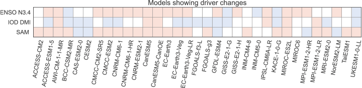
Fig. 1 shows that all 33 models show a large change in at least one driver. Nineteen models show a large increase in overall N3.4 amplitude (‘ENSO N3.4’ row), with five showing a large decrease. Nine models show little to no change. Fifteen models exhibit a large decrease in overall DMI amplitude (‘IOD DMI’ row), with 6 models showing a large increase, and 12 models showing small or no change. For SAM, 22 models exhibit a large amplitude increase. Only five models exhibit a large amplitude decrease, and six models exhibit little or no change. The most common changes therefore correspond to an increase in ENSO and SAM variability, and a decrease in IOD variability. These changes are estimated to be statistically significant at the 99, 99.9 and 92% levels respectively according to a two-tailed binomial test.
To gauge if the interrelationship between these changes to ENSO, IOD and SAM are linked, we try to identify if the changes are correlated. If we assign +1 to an increase, −1 to a decrease and 0 to little or no change in each model (focusing here only on the direction of change, not the magnitude), then we can calculate the correlation coefficient between the sign of the driver changes. The correlation between the sign of changes in ENSO and the IOD is 0.37. The correlation between the sign of changes in ENSO and SAM is −0.01. The correlation between the sign of changes in the IOD and SAM is 0.14. This indicates that the changes in SAM occur independently of the other two drivers, whereas the changes in the IOD are weakly (and positively) correlated with changes to ENSO.
These results help to explain why only 5 of the 33 models (15%) exhibit an increase in the variability of both ENSO and SAM, accompanied by a decrease in IOD variability. So, although the most common responses are increases in ENSO SST variability (in 58% of models), an increase in SAM variability (in 67% of models) and a decrease in IOD variability (in 45% of models), only 15% of the models exhibit all three of these changes.
For ease of presentation, for the rest of the study, we focus on the most frequently evident change in the models. To do this, we restrict attention to the 19 models that exhibit an increase in ENSO variability when discussing changes in ENSO teleconnections, the 15 models that exhibit a decrease in IOD variability when discussing changes in IOD teleconnections, and the 22 models that exhibit an increase in SAM variability when discussing SAM teleconnection changes. We refer to these groups of models as the ‘representative models’ in the rest of this study. The rainfall changes evident in the remaining ‘minority’ groups of models are shown in Supplementary Fig. S3–S8.
3.2. Overall teleconnection changes
Over the 1950–2005 period, observed springtime rainfall in large parts of central and eastern Australia was significantly correlated with Niño3.4 and the DMI, and rainfall in southern and eastern Australia was correlated with the SAM index (not shown). This correlation is reasonably well simulated in the CMIP6 multi-model mean for ENSO and IOD, but less so for SAM (Chung et al. 2023). Although Chung et al. (2023) used only the first ensemble member for each model, we find similar results using all available ensemble members from the same models.
Fig. 2 shows the SON teleconnection pattern (i.e. the linear regression coefficient between Niño3.4, DMI and SAM indices, and rainfall) for Historical and SSP3-7.0 scenarios. For each driver, we use the subset of ‘representative models’ identified in the previous section. Fig. 2a shows a significant relationship between Niño3.4 and rainfall over north-eastern, central and south-eastern Australia in the historical late 20th Century period. Here, significance is measured as any grid point in which >70% of models exhibit a regression coefficient that is significant at the 90% level using a t-test. Under SSP3-7.0, the regions of significance extend over northern and eastern Australia, strengthening slightly in the north and in southern Victoria (Fig. 2d). Fig. 2g shows the change in teleconnections (late 21st Century minus late 20th Century). This is broadly consistent with McGregor et al. (2022), who analysed the global projected change in DJF ENSO teleconnections, finding a strengthening in the ENSO teleconnections to north-eastern Australian rainfall.
Multi-model mean of linear regression slopes between SON mean rainfall and (a) SON Niño3.4, (b) SON DMI, (c) SON SAM indices for 1950–2014 (late 20th Century) using the subset of ‘representative models’ for each driver. (d–f) The same, but for 2035–2099 (late 21st Century) under the SSP3-7.0 scenario. (g–i) Late 21st Century minus late 20th Century regression slopes. To ensure each model is weighted equally, the multi-ensemble mean is used for models with more than one ensemble member. In (a–f), maps are stippled where more than 70% of models show a regression coefficient that is significant at the 90% level according to a t-test.
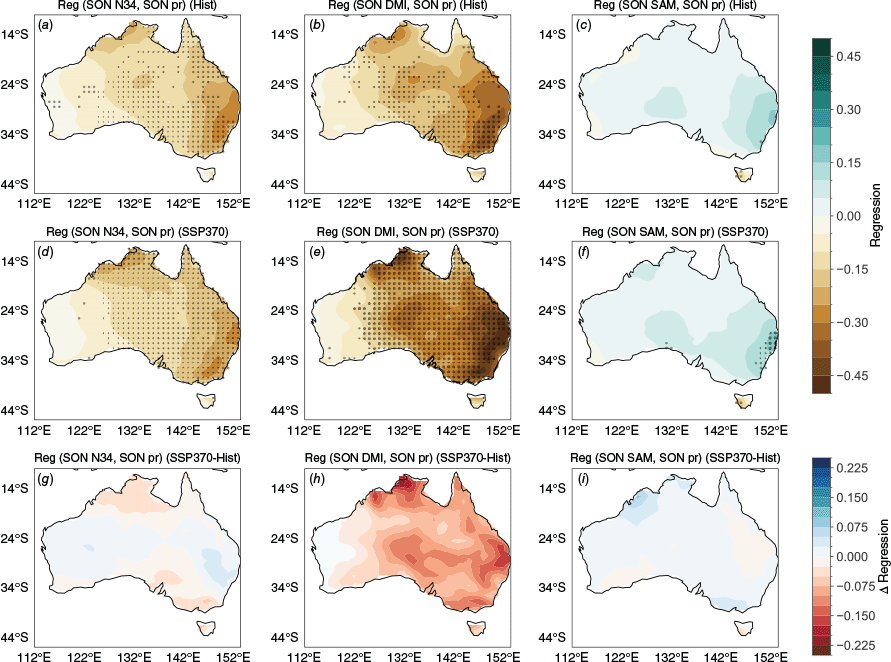
The IOD teleconnection also is projected to strengthen from late 20th to late 21st Centuries, with a band of significant regression coefficients extending from north-western to south-eastern Australia in the late 20th Century (Fig. 2b) expanding to cover a larger fraction of central and northern Australia in late 21st Century (Fig. 2e, h). It is interesting to note that IOD teleconnections are projected to strengthen even in this subset of models that project an overall weakening of the DMI. This may be linked to several contributing factors. Firstly, Wang G et al. (2024) showed that models project increased SST variability in the tropical Indian Ocean that is not fully captured by the DMI owing to asymmetric responses in the eastern and western regions of the Indian Ocean. Secondly, rainfall during IOD years is closely related to the strengthening ENSO teleconnections, as many IOD and ENSO events co-occur. Thirdly, it is likely that in a warmer world, SST variability in the tropics can inducea stronger rainfall response (e.g. Pendergrass 2020). In Section 3.4, we take a closer look at the asymmetric rainfall response during pIOD and nIOD phases.
For SAM, as noted in Chung et al. (2023), there is generally a poorer representation of teleconnections and a larger amount of inter-model spread. In this subset of models, in late 20th Century, the only significant teleconnections are found in western Tasmania (Fig. 2c). In late 21st Century, this teleconnection strengthens and extends to the south-eastern coast of Australia (Fig. 2f, i).
The differences between late 21st and late 20th Centuries regression slopes are shown in Fig. 2g–i, highlighting the regions in which the relationship strengthens significantly. For ENSO and IOD, these are largest in northern Australia. The representative models therefore indicate that ENSO, IOD and SAM teleconnections are likely to strengthen under SSP3-7.0 in many regions, particularly over central and eastern Australia. This is true even in the case of the IOD, which is projected to weaken.
We now consider two questions:
How does the total rainfall (i.e. including the trend), averaged over years in a particular phase, change in these subsets of models?
How do the driver-related rainfall anomalies change?
Here, we present the MMEM changes to rainfall totals and anomalies averaged over ENSO, IOD and SAM phases. For ease of presentation, we show only the ‘representative’ model MMEM for each driver discussed in Section 3. For reference, MMEM SON rainfall changes for all years are shown in Supplementary Fig. S1a, and late 20th Century anomalies for each phase of ENSO, IOD and SAM are shown in Supplementary Fig. S1b–g.
3.3. Stronger ENSO events
From Section 3.1, we showed that the MMEM of the subset of ‘representative models’ for ENSO events indicates stronger ENSO activity, or, more precisely, a larger amplitude in N3.4 SST swings. The MMEM rainfall projections for these 19 models are shown in Fig. 3, separated into El Niño (EN) and La Niña (LN) years. We present the rainfall projections in two ways: the mean-state change (Fig. 3a, c), and the change in anomalies during EN and LN years (Fig. 3b, d). The mean-state change is simply the late 21st–late 20th Century difference in rainfall averaged over all years in a particular phase, for example during EN or LN years. The change in anomalies is the late 21st–late 20th Century difference in EN and LN anomalies. For example, EN anomalies in the late 21st Century period would be the rainfall during EN years minus the mean rainfall for all years in late 21st Century. EN anomalies in the late 20th Century period would be the same, but relative to the late 20th Century climatology. The change in anomalies is then the difference in these two quantities. For reference, late 20th Century anomalies for EN and LN years are shown in Supplementary Fig. S1b, c and late 20th Century correlations between rainfall and N3.4 are shown in Supplementary Fig. S2a, b.
(a) SSP3-7.0 (late 21st Century) – historical (late 20th Century) mean-state change in total SON rainfall, averaged over El Niño years only. (b) SSP3-7.0 (late 21st Century) – historical (late 20th Century) change in SON rainfall anomalies, averaged over El Niño years only. (c, d) The same, but for La Niña years. Maps show the multi-model mean of the 19 ‘representative’ models that project stronger ENSO variability. Maps are stippled where over 70% of the models agree on the sign of the change.
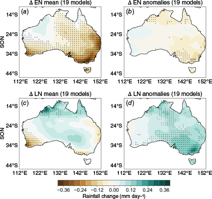
The ‘representative’ models project a significant mean-state drying over south-west Western Australia (SWWA) and southern Victoria during SON in both EN and LN phases (Fig. 3a, c). During EN years, there is also a significant mean-state drying over most of southern and eastern Australia (Fig. 3a). EN-related rainfall deficits are projected to intensify over south-eastern Australia and over the Kimberley region in north-west Australia (Fig. 3b). During LN years, the mean-state drying over SWWA and southern Victoria is accompanied by a rainfall increase around the Kimberley region (Fig. 3c). LN-related anomalies are projected to become wetter over much of southern Australia and parts of the Northern Territory (Fig. 3d).
The ‘minority’ models corresponding to a decrease in ENSO variability (five models), or little to no change (nine models) are shown in Supplementary Fig. S3–S4. The significant mean-state drying over SWWA and southern Victoria appears in all groups of models, though other regional mean-state changes differ between groups. The EN- and LN-related anomalies also differ, with the ‘weaker ENSO’ group generally exhibiting overall opposite sign changes from those shown in Fig. 3, as expected. The ‘no change’ group exhibits wetter LN-related anomalies but little change in EN-related anomalies, reflecting a general strengthening of teleconnections especially during LN years.
In the ‘representative’ models corresponding to stronger ENSO variability, the overall drying during EN and wetter conditions during LN years are consistent with a stronger driving ENSO signal from the Pacific, and consistent with the strengthened teleconnections shown in Fig. 2a, d. We note also that the mean-state drying over SWWA and southern Victoria is a robust trend that occurs regardless of driver change or phase, and is likely dominated by the climate change signal. SWWA is not a region that is heavily influenced by ENSO (Fig. 2a), so it is unsurprising that the mean-state drying over this region occurs in all models. However, southern Victorian rainfall is significantly correlated with ENSO, so it is notable that the mean-state drying occurs in all models, even under strengthened teleconnections to ENSO in which LN-induced rainfall increases; see discussion below.
3.4. Weaker IOD events
In contrast to ENSO, for the IOD, the 15 ‘representative models’ project weaker events. In these projections, both pIOD and nIOD years exhibit mean-state drying over much of western and eastern Australia, and a slight rainfall increase over the Kimberley region (Fig. 4a, c). pIOD years exhibit more widespread mean-state drying over eastern Australia (Fig. 4a). From Fig. 4a, c and Supplementary Fig. S5–S6, we can see again that the mean-state drying over SWWA and southern Victoria arises regardless of driver change or phase, noting that SWWA is also a region that is not typically heavily influenced by the IOD. The mean-state rainfall increase over the Kimberley region during pIOD years also occurs in all model groups.
(a) SSP3-7.0 (late 21st Century) – historical (late 20th Century) mean-state change in total SON rainfall, averaged over positive IOD years only. (b) SSP3-7.0 (late 21st Century) – historical (late 20th Century) change in SON rainfall anomalies, averaged over positive IOD years only. (c, d) The same, but for negative IOD years. Maps show the multi-model mean of the 15 ‘representative’ models that project weaker IOD variability. Maps are stippled where over 70% of the models agree on the sign of the change.
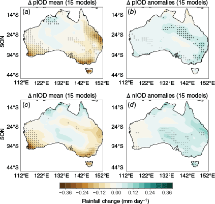
Late 20th Century rainfall anomalies and rainfall–DMI correlation for pIOD and nIOD years are shown in Supplementary Fig. S1d, e and S2c, d respectively. In a future with weaker IOD events, we would typically expect IOD-related rainfall anomalies to weaken, i.e. that pIOD anomalies would be less dry and nIOD anomalies would be less wet. Although this is certainly true of pIOD anomalies, nIOD anomaly changes in fact strengthen. The blue shading in Fig. 4b indicates that pIOD rainfall anomalies, which are typically dry, become less dry over parts of central and south-eastern Australia. However, nIOD-related anomalies become wetter (Fig. 4d), which reflects an asymmetry in the response to IOD change. It is also important to recall that the IOD and ENSO are strongly correlated in observations and models, so nIOD years often co-occur with LN years. The strengthening of wet anomalies during nIOD years despite the weakening of IOD variability may be related to the strengthened teleconnections to LN, given that many LN and nIOD years co-occur.
The ‘minority’ models corresponding to a strengthening IOD (6 models) and little to no change (12 models) show similar results for nIOD-related anomalies, which are increased rainfall in the south-east (Supplementary Fig. S5d, S6d). For pIOD-related anomalies, the ‘stronger IOD’ models show increased drying over the south-east and less drying in the west (Supplementary Fig. S5c), with similar but weaker patterns for the ‘no change’ models (Supplementary Fig. S6c). For pIOD years, changes are broadly of opposite sign to those exhibited by the ‘representative’ models.
3.5. Stronger SAM variability
Although there is limited model skill in capturing SAM teleconnections to Australia, SAM variability is projected to strengthen in 22 models, which is the most robust change out of all three drivers (Fig. 1). Similarly to ENSO and IOD, the significant mean-state changes for both positive SAM (pSAM) and negative SAM (nSAM) regions correspond to drying over SWWA, southern Victoria and southern Queensland (Fig. 5a, c). For nSAM years, the drying is more widespread across eastern Australia and there is a mean-state rainfall increase over the Cape York region (Fig. 5c). Neither pSAM- nor nSAM-related anomalies exhibit any widespread significant change (Fig. 5b, d), with only increased drying over the Kimberley region in nSAM years being stippled in Fig. 5d.
(a) SSP3-7.0 (late 21st Century) – Historical (L20C) mean-state change in total SON rainfall, averaged over positive SAM years only. (b) SSP3-7.0 (late 21st Century) – Historical (L20C) change in SON rainfall anomalies, averaged over positive SAM years only. (c, d) The same, but for negative SAM years. Maps show the multi-model mean of the 22 models that fall under the ‘most likely’ SAM-change pathway (stronger SAM variability in SON). Maps are stippled where over 70% of the models agree on the sign of the change.
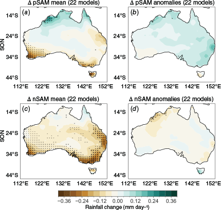
Only five models project a weakening of SAM and four project little to no change. The mean-state and anomaly changes for these ‘minority’ groups of models exhibit varying regional responses (Supplementary Fig. S7–S8); however, the mean-state drying over SWWA again remains a robust response in all model groups. The ‘weaker’ SAM models generally show wetter anomalies in both phases of SAM, whereas the ‘no change’ SAM models show drier anomalies over the south-east in both phases of SAM.
For reference, late 20th Century rainfall anomalies in pSAM and nSAM years are shown in Supplementary Fig. S1f, g, with the late 20th Century correlations between rainfall and SAM index shown in Supplementary Fig. S2e, f. Given the relatively weak change in SAM teleconnections in the ‘representative’ models (Fig. 5b, d), it is therefore unclear if or how a strengthening of SAM variability during SON might affect rainfall variability. It is also worth noting that the SAM–ENSO relationship, which modulates the teleconnection of SAM with Southern Hemispheric rainfall, is not well captured in models (Lim et al. 2016). However, the mean-state changes over southern Australia clearly reflect the dominance of the mean-state climate change signal over any forced changes in internal variability.
Previous studies have shown that models project an overall drying over Australia during winter and spring (Delage and Power 2020; CSIRO and Bureau of Meteorology 2024), particularly over SWWA (Delage and Power 2020; McKay et al. 2023; Rauniyar et al. 2023) and southern Victoria (Rauniyar and Power 2023). This is evident in Fig. 3–5, and Supplementary Fig. S3–S8, which show that regardless of the direction of projected driver changes, or phases, SWWA and southern Victoria exhibit a significant drying signal. These projections indicate that the climate-change signal in these regions dominates the mean-state change in springtime rainfall. That is, regardless of how the variability of ENSO, IOD or SAM might change, over 70% of models project drying in the late 21st Century period in these regions. This is consistent with the CMIP5 results obtained by Delage and Power (2020) in their examination of the combined impact of global warming and ENSO on winter and spring rainfall over Australia.
3.6. Concurrent ENSO and IOD events
Given the impacts of EN + pIOD and LN + nIOD events on Australian rainfall are amplified when these phases co-occur, which they often do (e.g. Ummenhofer et al. 2011; Holgate et al. 2022), it is of interest to present similar rainfall projections for concurrent events. However, the projected strengthening in ENSO events and weakening in IOD events means it is not immediately clear how modelled rainfall might respond to future concurrent events. Therefore, in this section, we turn our attention to changes to the frequency (i.e. number) of concurrent events rather than the amplitude of the indices. Chung et al. (2024) compared the frequency of concurrent events in late 20th and 21st Centuries in each model, finding that there were almost no statistically significant changes in occurrences of concurrent events under SSP3-7.0. Only the LN + nIOD + nSAM combination exhibited a statistically significant increase.
As there is no clear majority in the direction of change, we present here rainfall changes associated with both EN + pIOD and LN + nIOD increases and decreases (combining both phases of SAM). We present MMEM mean-state changes and anomaly changes for four subgroups of models, i.e. those that project an increase or decrease in EN + pIOD and an increase or decrease LN + nIOD events. We select only models that exhibit a frequency change of >0.5 s.d. across all models (Fig. 6a). In doing this, there are 15 out of 33 models that show increases, and 10 that show decreases in EN + pIOD events (with eight models showing little to no change in frequency). By contrast, there are eight models each showing an increase in LN + nIOD and seven showing a decrease in LN + nIOD events (and 18 models showing little to no change). Note that in Fig. 6a, models with little to no change in either EN + pIOD or LN + nIOD are not listed.
Top row (a): models showing projected MMEM increases (red) and decreases (blue) in the frequency of EN + pIOD events and LN + nIOD events. Only models with an amplitude change of over 0.5 s.d. across all models are coloured. Models are listed in alphabetical order. Middle row (b–e): concurrent EN + pIOD events. (b) Projected mean-state change in total rainfall, averaged over EN + pIOD years, for models showing a large frequency increase in EN + pIOD events. (c) Projected change in rainfall anomalies, averaged over EN + pIOD years, for models showing a large frequency increase in EN + pIOD events. (d) The same as (a) but for models showing a decrease in EN + pIOD events. (e) The same as (c) but for models showing a decrease in EN + pIOD events. Bottom row (f–i): the same, but for LN + nIOD events and for LN years only. Projected changes are shown for SSP3-7.0 (late 21st Century) – historical (late 20th Century) scenarios, for SON rainfall. Maps are stippled where over 70% of the models agree on the sign of the change.
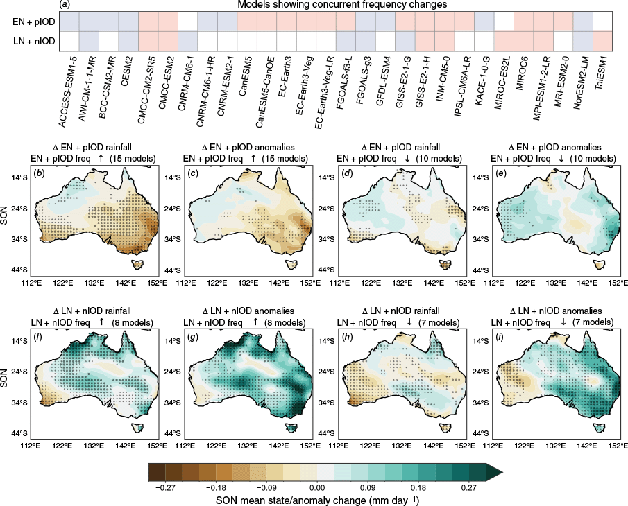
Fig. 6b–i shows the MMEM mean-state change (Fig. 6b, d, f, h) and anomaly changes (Fig. 6c, e, g, i) during concurrent EN + pIOD and LN + nIOD years associated with increases and decreases of EN + pIOD and LN + nIOD events. In the models that project an increase in EN + pIOD events, EN + pIOD years exhibit a mean-state drying over much of southern, central and eastern Australia, largest around SWWA and south-eastern Australia (Fig. 6b). (EN + pIOD)-related anomalies for these models show intensified drying over central and south-eastern Australia (Fig. 6c). This intensified drying over the south-east is consistent with what is expected from an increase in EN + pIOD events. The models that project a decrease in EN + pIOD also exhibit significant, though weaker, mean-state drying over regions covering SWWA, southern Victoria and south-eastern Queensland (Fig. 6d). The (EN + pIOD)-related anomalies for these models show wetter, or less dry, anomalies (indicated by blue shading) over parts of western and eastern Australia (Fig. 6e). The weaker anomalies seen here are broadly consistent with a weaker model response to fewer EN + pIOD events.
For LN + nIOD years, an increase in LN + nIOD events corresponds to a wetter mean state over northern Australia but still drying over SWWA (Fig. 6f). The LN-related anomalies for these models show an intensification of the wet anomalies over most of the country, particularly over the south-eastern and north-western regions (Fig. 6g). Again, this is consistent with what is expected from an increase in the rain-promoting phases of the drivers. The models showing a decrease in LN + nIOD events show mean-state drying over much of WA, with mixed changes elsewhere (Fig. 6h). (LN + pIOD)-related anomalies in these models still show an intensification of wet anomalies over much of eastern Australia, but drier anomalies over WA (Fig. 6i). Although there are fewer driving LN + nIOD events, the increase in wet anomalies over eastern Australias indicates that the future events that do occur have a stronger impact, which is consistent with the increase in teleconnection strength in these regions associated with stronger ENSO variability.
Although there is a clear lack of consensus on future changes to the frequency of concurrent ENSO and IOD phases, these results provide an indication of what the current generation of models project for either sign of change. More work is required to quantify the amplitude changes of these events as well as a detailed analysis of asymmetry in the responses to positive and negative phases.
3.7. Consecutive ENSO and IOD events
In recent years, consecutive (back-to-back) events such as the double ENs and pIODs of 2018–2019 (e.g. Wang and Cai 2020) and triple LNs and nIODs of 2020–2022 have also had major impacts on SON Australian rainfall (e.g. Huang et al. 2024). In this section, we identify all occurrences of two or more back-to-back EN, LN, pIOD and nIOD events and compare the projected rainfall changes for these events. For each back-to-back event in each model, the mean rainfall, or rainfall anomalies, averaged over the 2 years is calculated. This is then averaged over the whole period.
Mean-state changes and changes to anomalies are shown in Fig. 7 for consecutive EN (a, b), LN (c, d), pIOD (e, f) and nIOD (g, h) events. Chung et al. (2024) found no significant changes in any of these events under SSP3-7.0, so in this section, we present the MMEM of all 33 models. The mean-state changes for all four events, once again, display the strongest drying over SWWA and southern Victoria. For consecutive EN years, there is increased mean-state drying over much of south-west and eastern Australia (Fig. 7a). A weak response in the rainfall anomalies is seen, with some model consensus on increased drying in small parts of Victoria and the Kimberley region (Fig. 7b). Consecutive LN years show a mean-state increase over the Kimberley region and Cape York coast in addition to the drying in the south mentioned above (Fig. 7c). There is also a weak intensification of wet anomalies over parts of the south-east and north of the country (Fig. 7d).
Top row: (a) projected mean-state change in total rainfall, averaged over consecutive EN years, for all models. (b) Projected change in rainfall anomalies, averaged over consecutive years, for all models. (c, d) The same as (a, b) but for consecutive LN events. Bottom row: (e–h) the same as (a–d) but for consecutive pIOD (e, f), and nIOD (g, h) events. Projected changes are shown for SSP3-7.0 (late 21st Century) – historical (late 20th Century) scenarios, for SON rainfall. Maps are stippled where over 70% of the models agree on the sign of the change.
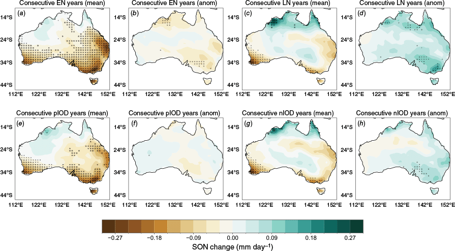
Consecutive pIOD and nIOD events display largely similar, albeit slightly weaker, responses to the EN and LN cases respectively. Consecutive pIOD years show mean-state drying over the south and eastern coast (Fig. 7e), with no model consensus anywhere on anomaly changes (Fig. 7f). Consecutive nIOD events show the mean-state drying to the south and increased rainfall over the far north (Fig. 7g), with models only agreeing on larger wet anomalies over a small part of Victoria (Fig. 7h).
These results suggest that the overall drying trend in SWWA, southern Victoria and Tasmania are a response to the changes in the mean state. Consecutive EN years would reinforce these dry conditions in future, whereas consecutive LN years would somewhat alleviate the mean-state drying. South-eastern Australia may therefore need to rely more on isolated and consecutive LN events in water management planning activities.
4.Summary and conclusions
This study identifies the subset of models that exhibit a majority consensus on how the strength of ENSO, IOD and springtime SAM is projected to change in the late 21st Century, as shown in Chung et al. (2024). The majority of models show a strengthening of ENSO and SAM variability and a weakening of the IOD, as measured by the DMI. For each subset of models showing these driver changes, we then present the associated mean-state change and change to anomalies for SON rainfall in the positive and negative phases of the drivers.
Although the changes to ENSO, IOD and SAM variability are largely independent of each other, there is a weak positive relationship between the sign of model-to-model changes in the IOD and ENSO. However, the projected changes in the sign of changes of SAM occur independently of projected changes to both ENSO and the IOD.
In terms of mean-state changes, the drying trend over SWWA and southern Victoria, identified in previous studies (Rauniyar and Power 2023; McKay et al. 2023), occurs in all driver phases and common combinations of driver phases, regardless of the sign of change of the drivers. In many phases, this drying also spans much of southern and eastern Australia. This indicates that the impacts of mean-state climate change are much larger than those linked to changes in the intensity of internal variability associated with the three drivers. This is consistent with earlier research using models of the CMIP5 that focussed on climate change and ENSO variability (Power and Delage 2018). Stronger ENSO and SAM in models are associated with more widespread drying during EN and nSAM years in the future, compared with LN and pSAM. The models that project weaker IOD also exhibit widespread mean-state drying during pIOD years, and to a lesser extent during nIOD years.
Models also show agreement that under stronger ENSO events, EN- and LN-related anomalies (relative to the late 21st Century climatology) are projected to strengthen over parts of south-eastern Australia. By contrast, with weaker IOD events, pIOD-related anomalies become less dry over most south-eastern Australia. There is almost no model consensus for rainfall change for pSAM, or nSAM-related rainfall anomalies in SON. For SAM, this is related to the very limited skill in the simulation of the teleconnection to Australian rainfall.
We then briefly investigated the rainfall changes associated with increases or decreases in concurrent EN + pIOD and LN + nIOD events. Increased EN + pIOD events are associated with a drier mean state over most of central and eastern Australia during EN + pIOD years. Models that project decreased EN + pIOD events also exhibit drying during these events but to a smaller spatial extent. Models that project increased LN + nIOD years are associated with increased rainfall over northern Australia. This rainfall increase is also seen, but to a smaller spatial extent in the models that show a decrease in LN + nIOD years.
The change in (EN + pIOD)- and (LN + nIOD)-related rainfall anomalies in models that show an increase in the frequency of concurrent events behaves as expected, with a widespread intensification of dry and wet anomalies respectively. In the models that project a decrease in the frequency of EN + pIOD events, the rainfall anomalies are more mixed, with less drying over western and eastern Australia. The models that project a decrease in the frequency of LN + nIOD events still display an increase in wet anomalies, though confined to eastern Australia.
We also examined the changes to rainfall associated with consecutive multi (i.e. double or more) EN, LN, pIOD and nIOD events. We find that mean rainfall changes associated with the dry-conducive drivers (EN and pIOD) exhibit more widespread drying across the south and east, whereas the changes associated with rainfall-promoting drivers (LN and nIOD) exhibit increased rainfall over the far north. Very little model agreement is seen in the rainfall anomalies. Although these projections are a first step towards understanding the rainfall changes associated with concurrent and consecutive drivers, it is important to reiterate the large model spread in the projected changes to the driver phases discussed above. This uncertainty limits the confidence in the associated rainfall projections. Further work is required to quantify these confidence limits.
The conclusions drawn from this section are dependent on the models’ skill in simulating the drivers and their teleconnections with Australian rainfall. There are known biases in the CMIP6 mean state and representation of the drivers that can affect these projections, such as the cold tongue bias, or some models having an overly biennial ENSO or overly strong IOD (e.g. Grose et al. 2020; McKenna et al. 2020). Additionally, as noted in Chung et al. (2023), the extremely large inter- and intra- model spread in simulating Australian rainfall teleconnections remains a large source of uncertainty. In the present study, we have weighted all models and ensemble members equally, regardless of skill. The main advantage of this approach is that it more fully samples the large range of internal variability in the climate system, which may be missed by using a smaller sub-sample of models. Other approaches, such as model selection based on certain criteria, may be better suited for projections based on specific physical processes (e.g. Delage and Power 2020; Geng et al. 2023). For model selection for regional downscaling purposes, it may be desirable to select only a few models that sample a range of possible futures (e.g. Grose et al. 2023). Using an ensemble of models also means that there could be a range of mechanisms that are responsible for projected rainfall changes. Future work and numerical experiments could investigate the details of the physical processes driving these teleconnection changes and model consensus on these processes. For example, changes to mean rainfall could be related to eastward shifts of the Pacific–South American pattern (Cai et al. 2021).
It is also important to note that ENSO, IOD and SAM variability constitute only a fraction of total rainfall variability (Hobeichi et al. 2024). These modes, and their impacts on Australian rainfall variability, are also modulated regionally by shorter time-scale and local processes such as the Madden–Julien Oscillation, moisture advection from the surrounding seas, land–atmosphere feedbacks and synoptic systems such as blocking highs and cut-off lows (Sharmila and Hendon 2020; Holgate et al. 2022, 2025; Cowan et al. 2023; Gillett et al. 2023; Huang et al. 2024). However, it is still of great value to understand the rainfall changes associated with these drivers, as the drivers hold some predictive capability (up to 50% in some regions) for seasonal rainfall variability, particularly in spring. On longer time-scales, the Interdecadal Pacific Oscillation also modulates the strength of these teleconnections (Arblaster et al. 2002; Power et al. 2006; Heidemann et al. 2024). The interplay between naturally occurring variability at different temporal and spatial scales, as well as the evolving climate change forcing, remain a complex problem for global and regional climate models to address.
Our results suggest that in future, EN and pIOD events will tend to exacerbate the drying projections associated with the mean-state changes, particularly in southern Australia in springtime. By contrast, LN and nIOD events would alleviate the magnitude of the mean-state drying, although they do not reverse the drying in the southern parts of the country. Considering these projections, economic sectors dependent on seasonal rainfall (e.g. water management, agriculture, tourism, fire management) in SWWA and Victoria will need to adapt to reduced springtime rainfall. To further constrain projections, more work is needed to fully explore possible changes to the interaction between drivers and their associated teleconnections, under a range of plausible future scenarios.
Data availability
All CMIP6 data used in this study are publicly available from https://esgf.nci.org.au/projects/esgf_nci/.
Conflicts of interest
Andréa Taschetto is an Associate Editor of the Journal of Southern Hemisphere Earth Systems Science (JSHESS). Despite this relationship, Andréa took no part in the review and acceptance of this manuscript, in line with the publishing policy. JSHESS encourages its editors to publish in the journal and they are kept totally separate from the decision-making processes for their manuscripts. The authors have no further conflicts of interest to declare.
Declaration of funding
This study was supported with funding from the Australian Government’s National Environmental Science Program. This research was undertaken with the assistance of resources and services from the National Computational Infrastructure (NCI), which is supported by the Australian Government.
Acknowledgements
We acknowledge the World Climate Research Programme, which, through its Working Group on Coupled Modelling, coordinated and promoted CMIP6. We thank the climate modelling groups for producing and making available their model output, the Earth System Grid Federation (ESGF) for archiving the data and providing access, and the multiple funding agencies who support CMIP6 and ESGF. We thank Danielle Udy, Rajashree Naha and David Jones for helpful reviews of the manuscript.
References
An SI, Park HJ, Kim SK, et al. (2023) Main drivers of Indian Ocean Dipole asymmetry revealed by a simple IOD model. npj Climate and Atmospheric Science 6, 93.
| Crossref | Google Scholar |
Arblaster J, Meehl G, Moore A (2002) Interdecadal modulation of Australian rainfall. Climate Dynamics 18, 519-531.
| Crossref | Google Scholar |
Baldwin MP, Ayarzagüena B, Birner T, Butchart N, Butler AH, Charlton-Perez AJ, et al. (2021) Sudden stratospheric warmings. Reviews of Geophysics 59, e2020RG000708.
| Crossref | Google Scholar |
Bonfils CJW, Santer BD, Phillips TJ, Marvel K, Leung LR, Doutriaux C, Capotondi A (2015) Relative contributions of mean state shifts and ENSO-driven variability to precipitation changes in a warming climate. Journal of Climate 28, 9997-10013.
| Crossref | Google Scholar |
Cai W, van Rensch P, Cowan T, Sullivan A (2010) Asymmetry in ENSO teleconnection with regional rainfall, its multidecadal variability, and impact. Journal of Climate 23, 4944-4955.
| Crossref | Google Scholar |
Cai W, van Rensch P, Cowan T, Hendon HH (2011) Teleconnection pathways of ENSO and the IOD and the mechanisms for impacts on Australian rainfall. Journal of Climate 24, 3910-3923.
| Crossref | Google Scholar |
Cai W, Santoso A, Collins M, et al. (2021) Changing El Niño–Southern Oscillation in a warming climate. Nature Reviews Earth & Environment 2, 628-644.
| Crossref | Google Scholar |
Cai W, Ng B, Wang G, et al. (2022) Increased ENSO sea surface temperature variability under four IPCC emission scenarios. Nature Climate Change 12, 228-231.
| Crossref | Google Scholar |
Chung CTY, Power S (2017) The non-linear impact of El Niño, La Niña and the Southern Oscillation on seasonal and regional Australian precipitation. Journal of Southern Hemisphere Earth Systems Science 67(1), 25-45.
| Crossref | Google Scholar |
Chung C, Boschat G, Taschetto A, Narsey S, McGregor S, Santoso A, Delage F (2023) Evaluation of seasonal teleconnections to remote drivers of Australian rainfall in CMIP5 and CMIP6 models. Journal of Southern Hemisphere Earth Systems Science 73, 219-261.
| Crossref | Google Scholar |
Chung CTY, Power SB, Boschat G, Gillett ZE, Narsey S (2024) Projected changes to characteristics of El Niño–Southern Oscillation, Indian Ocean Dipole, and Southern Annular Mode events in the CMIP6 models. Earth’s Future 12, e2024EF005166.
| Crossref | Google Scholar |
CORDEX (2025) CORDEX experiment design for dynamical downscaling of CMIP6. Zenodo 2025, version v2 [Preprint, published 28 April 2025].
| Crossref | Google Scholar |
Cowan T, Wheeler MC, Marshall AG (2023) The combined influence of the Madden–Julian Oscillation and El Niño–Southern Oscillation on Australian rainfall. Journal of Climate 36(2), 313-334.
| Crossref | Google Scholar |
CSIRO and Bureau of Meteorology (2024) State of the Climate 2024. (Government of Australia) Available at https://www.csiro.au/en/research/environmental-impacts/climate-change/state-of-the-climate
Delage FPD, Power SB (2020) The impact of global warming and the El Niño–Southern Oscillation on seasonal precipitation extremes in Australia. Climate Dynamics 54, 4367-4377.
| Crossref | Google Scholar |
Deng K, Azorin-Molina C, Yang S, Hu C, Zhang G, Minola L, Chen D (2022) Changes of Southern Hemisphere westerlies in the future warming climate. Atmospheric Research 270, 106040.
| Crossref | Google Scholar |
Devanand A, Falster GM, Gillett ZE, et al. (2024) Australia’s tinderbox drought: an extreme natural event likely worsened by human-caused climate change. Science Advances 10, eadj3460.
| Crossref | Google Scholar | PubMed |
Domeisen DIV, Butler AH (2020) Stratospheric drivers of extreme events at the Earth’s surface. Communications Earth & Environment 1, 59.
| Crossref | Google Scholar |
Domeisen DIV, Butler AH, Charlton-Perez AJ, Ayarzagüena B, Baldwin MP, Dunn-Sigouin E, et al. (2020) The role of the stratosphere in subseasonal to seasonal prediction: 1. Predictability of the stratosphere. Journal of Geophysical Research: Atmospheres 125, e2019JD030920.
| Crossref | Google Scholar |
Endris HS, Lennard C, Hewitson B, et al. (2019) Future changes in rainfall associated with ENSO, IOD and changes in the mean state over eastern Africa. Climate Dynamics 52, 2029-2053.
| Crossref | Google Scholar |
Eyring V, Bony S, Meehl GA, Senior CA, Stevens B, Stouffer RJ, Taylor KE (2016) Overview of the Coupled Model Intercomparison Project Phase 6 (CMIP6) experimental design and organization. Geoscientific Model Development 9, 1937-1958.
| Crossref | Google Scholar |
Geng T, Jia F, Cai W, et al. (2023) Increased occurrences of consecutive La Niña events under global warming. Nature 619, 774-781.
| Crossref | Google Scholar | PubMed |
Gillett ZE, Taschetto AS, Holgate CM, Santoso A (2023) Linking ENSO to synoptic weather systems in eastern Australia. Geophysical Research Letters 50, e2023GL104814.
| Crossref | Google Scholar |
Gong D, Wang S (1999) Definition of Antarctic Oscillation Index. Geophysical Research Letters 26, 459-462.
| Crossref | Google Scholar |
Goyal R, Sen Gupta A, Jucker M, England MH (2021) Historical and projected changes in the Southern Hemisphere surface westerlies. Geophysical Research Letters 48, e2020GL090849.
| Crossref | Google Scholar |
Grose MR, Narsey S, Delage FP, Dowdy AJ, Bador M, Boschat G, et al. (2020) Insights from CMIP6 for Australia’s future climate. Earth’s Future 8, e2019EF001469.
| Crossref | Google Scholar |
Grose MR, Narsey S, Trancoso R, Mackallah C, Delage F, Dowdy A, Di Virgilio G, Watterson I, Dobrohotoff P, Rashid HA, Rauniyar S, Henley B, Thatcher M, Syktus J, Abramowitz G, Evans JP, Su C-H, Takbash A (2023) A CMIP6-based multi-model downscaling ensemble to underpin climate change services in Australia. Climate Services 30, 100368.
| Crossref | Google Scholar |
Hausfather Z (2025) An assessment of current policy scenarios over the 21st Century and the reduced plausibility of high-emissions pathways. Dialogues on Climate Change 2(1), 26-32.
| Crossref | Google Scholar |
Heidemann H, Cowan T, Power SB, et al. (2024) Statistical relationships between the Interdecadal Pacific Oscillation and El Niño–Southern Oscillation. Climate Dynamics 62, 2499-2515.
| Crossref | Google Scholar |
Hendon HH, Thompson DWJ, Wheeler MC (2007) Australian rainfall and surface temperature variations associated with the Southern Hemisphere Annular Mode. Journal of Climate 20, 2452-2467.
| Crossref | Google Scholar |
Hobeichi S, Abramowitz G, Sen Gupta A, et al. (2024) How well do climate modes explain precipitation variability? npj Climate and Atmospheric Science 7, 295.
| Crossref | Google Scholar |
Holgate C, Evans JP, Taschetto AS, Gupta AS, Santoso A (2022) The impact of interacting climate modes on east Australian precipitation moisture sources. Journal of Climate 35, 3147-3159.
| Crossref | Google Scholar |
Holgate C, Falster GM, Gillett ZE, et al. (2025) Physical mechanisms of drought development, intensification and termination: an Australia review. Communications Earth & Environment 6, 220.
| Crossref | Google Scholar |
Huang AT, Gillett ZE, Taschetto AS (2024) Australian rainfall increases during multi-year La Niña. Geophysical Research Letters 51, e2023GL106939.
| Crossref | Google Scholar |
Intergovernmental Panel On Climate Change (2023) ‘Climate Change 2021 – The Physical Science Basis: Working Group I Contribution to the Sixth Assessment Report of the Intergovernmental Panel on Climate Change.’ (Cambridge University Press) doi:10.1017/9781009157896
Kim SK, Park HJ, An SI, et al. (2024) Decreased Indian Ocean Dipole variability under prolonged greenhouse warming. Nature Communications 15, 2811.
| Crossref | Google Scholar | PubMed |
Liguori G, McGregor S, Singh M, Arblaster J, Di Lorenzo E (2022) Revisiting ENSO and IOD contributions to Australian precipitation. Geophysical Research Letters 49, e2021GL094295.
| Crossref | Google Scholar |
Lim E-P, Hendon HH (2015) Understanding the contrast of Australian springtime rainfall of 1997 and 2002 in the frame of two flavors of El Niño. Journal of Climate 28, 2804-2822.
| Crossref | Google Scholar |
Lim E-P, Hendon HH, Arblaster JM, Delage F, Nguyen H, Min S-K, Wheeler MC (2016) The impact of the Southern Annular Mode on future changes in Southern Hemisphere rainfall. Geophysical Research Letters 43, 7160-7167.
| Crossref | Google Scholar |
Lim E-P, Hendon HH, Butler AH, et al. (2021) The 2019 Southern Hemisphere stratospheric polar vortex weakening and its impacts. Bulletin of the American Meteorological Society 102, E1150-E1171.
| Crossref | Google Scholar |
Ma Y, Sun J, Dong T, et al. (2023) More profound impact of CP ENSO on Australian spring rainfall in recent decades. Climate Dynamics 60, 3065-3079.
| Crossref | Google Scholar |
MacLeod D, Kolstad EW, Michaelides K, Singer MB (2024) Sensitivity of rainfall extremes to unprecedented Indian Ocean Dipole events. Geophysical Research Letters 51, e2023GL105258.
| Crossref | Google Scholar |
McGregor S, Cassou C, Kosaka Y, Phillips AS (2022) Projected ENSO teleconnection changes in CMIP6. Geophysical Research Letters 49, e2021GL097511.
| Crossref | Google Scholar |
McKay RC, Boschat G, Rudeva I, Pepler A, Purich A, Dowdy A, Hope P, Gillett ZE, Rauniyar S (2023) Can southern Australian rainfall decline be explained? A review of possible drivers. WIREs Climate Change 14(2), e820.
| Crossref | Google Scholar |
McKenna S, Santoso A, Gupta AS, Taschetto AS, Cai W (2020) Indian Ocean Dipole in CMIP5 and CMIP6: characteristics, biases, and links to ENSO. Scientific Reports 10(1), 11500.
| Crossref | Google Scholar |
Meneghini B, Simmonds I, Smith IN (2007) Association between Australian rainfall and the Southern Annular Mode. International Journal of Climatology 27, 109-121.
| Crossref | Google Scholar |
Narsey SY, Brown JR, Colman RA, Delage F, Power SB, Moise AF, Zhang H (2020) Climate change projections for the Australian monsoon from CMIP6 models. Geophysical Research Letters 47, e2019GL086816.
| Crossref | Google Scholar |
Pendergrass AG (2020) The global-mean precipitation response to CO2-induced warming in CMIP6 models. Geophysical Research Letters 47, e2020GL089964.
| Crossref | Google Scholar |
Pepler A, Timbal B, Rakich C, Coutts-Smith A (2014) Indian Ocean Dipole overrides ENSO’s influence on cool season rainfall across the eastern seaboard of Australia. Journal of Climate 27, 3816-3826.
| Crossref | Google Scholar |
Perry SJ, McGregor S, Gupta AS, England MH (2017) Future changes to El Niño–Southern Oscillation temperature and precipitation teleconnections. Geophysical Research Letters 44, 10,608-10,616.
| Crossref | Google Scholar |
Perry SJ, McGregor S, Sen Gupta A, et al. (2020) Projected late 21st Century changes to the regional impacts of the El Niño–Southern Oscillation. Climate Dynamics 54, 395-412.
| Crossref | Google Scholar |
Power SB, Callaghan J (2016) Variability in severe coastal flooding, associated storms, and death tolls in southeastern Australia since the Mid-Nineteenth Century. Journal of Applied Meteorology and Climatology 55, 1139-1149.
| Crossref | Google Scholar |
Power SB, Delage FP (2018) El Niño–Southern Oscillation and associated climatic conditions around the world during the latter half of the Twenty-First Century. Journal of Climate 31, 6189-6207.
| Crossref | Google Scholar |
Power S, Haylock M, Colman R, Wang X (2006) The predictability of interdecadal changes in ENSO activity and ENSO teleconnections. Journal of Climate 19, 4755-4771.
| Crossref | Google Scholar |
Power S, Delage F, Chung C, Kociuba G, Keay K (2013) Robust Twenty-First-Century projections of El Niño and related precipitation variability. Nature 502, 541-545.
| Crossref | Google Scholar | PubMed |
Rauniyar SP, Power SB (2023) Past and future rainfall change in sub-regions of Victoria, Australia. Climatic Change 176, 92.
| Crossref | Google Scholar |
Rauniyar SP, Hope P, Power SB, et al. (2023) The role of internal variability and external forcing on southwestern Australian rainfall: prospects for very wet or dry years. Scientific Reports 13, 21578.
| Crossref | Google Scholar |
Riahi K, van Vuuren DP, Kriegler E, et al. (2017) The shared socioeconomic pathways and their energy, land use, and greenhouse gas emissions implications: an overview. Global Environmental Change 42, 153-168.
| Crossref | Google Scholar |
Risbey JS, Pook MJ, McIntosh PC, Wheeler MC, Hendon HH (2009) On the remote drivers of rainfall variability in Australia. Monthly Weather Review 137, 3233-3253.
| Crossref | Google Scholar |
Saji NH, Goswami BN, Vinayachandran PN, Yamagata T (1999) A dipole mode in the tropical Indian Ocean. Nature 401, 360-363.
| Crossref | Google Scholar | PubMed |
Sharmila S, Hendon HH (2020) Mechanisms of multiyear variations of Northern Australia wet-season rainfall. Scientific Reports 10(1), 5086.
| Crossref | Google Scholar |
Tozer CR, Risbey JS, Pook MJ, Monselesan DP, Irving DB, Ramesh N, Richardson D (2024) A tale of two Novembers: confounding influences on La Niña’s relationship with rainfall in Australia. Monthly Weather Review 152, 1977-1996.
| Crossref | Google Scholar |
Ummenhofer CC, England MH, McIntosh PC, Meyers GA, Pook MJ, Risbey JS, Gupta AS, Taschetto AS (2009) What causes southeast Australia’s worst droughts? Geophysical Research Letters 36, L04706.
| Crossref | Google Scholar |
Ummenhofer CC, Gupta AS, Briggs PR, et al. (2011) Indian and Pacific Ocean influences on southeast Australian drought and soil moisture. Journal of Climate 24, 1313-1336.
| Crossref | Google Scholar |
van Rensch P, Gallant AJE, Cai W, Nicholls N (2015) Evidence of local sea surface temperatures overriding the southeast Australian rainfall response to the 1997–1998 El Niño. Geophysical Research Letters 42, 9449-9456.
| Crossref | Google Scholar |
Wang G, Cai W (2020) Two-year consecutive concurrences of positive Indian Ocean Dipole and Central Pacific El Niño preconditioned the 2019/2020 Australian ‘Black Summer’ bushfires. Geoscience Letters: 7, 19.
| Crossref | Google Scholar |
Wang G, Cai W, Santoso A, et al. (2024) The Indian Ocean Dipole in a warming world. Nature Reviews Earth & Environment 5, 588-604.
| Crossref | Google Scholar |
Wang J, Sun S, Zu Y, Fang Y (2024) Increased frequency of consecutive positive IOD events under global warming. Geophysical Research Letters 51, e2024GL111182.
| Crossref | Google Scholar |