

Influence of landscape features on the distribution of the vulnerable frog species Mixophyes iteratus in the Tweed Valley, northern New South Wales, Australia
Gregory W. Lollback A * , Michele A. Lockwood B and David S. Hannah A
A
B
Abstract
Knowing more about the influence of landscape features on occurrence or abundance may aid in conservation management of the vulnerable frog species Mixophyes iteratus in Australia.
We aimed to understand how M. iteratus is influenced by landscape features and fill in the knowledge gap on species distribution within the Tweed Valley landscape of northern New South Wales.
The species was sampled at 40 stream-based transects spread across the Tweed Valley during three breeding seasons, from 2019 to 2022. Occupancy analysis and general additive models were used to investigate the relationship between landscape features and frog occurrence and maximum frog count, respectively. Landscape variables included elevation, proportion of vegetation cover, stream morphology, and distance to conservation reserves.
Mixophyes iteratus distribution was concentrated in the western half of the Tweed Valley, over a range of landscape features. Landscape features did not strongly affect distribution at specific scales or in general. There was some spatial clustering of maximum frog count, especially in large, forested areas in the south and south-west of the Tweed Valley. Detection rate was higher in this study when compared to a previous study with shorter transects.
Modelling suggests that M. iteratus occurred over a broad distribution within the western half of the Tweed Valley before broad scale clearing occurred. Species occurrence is wider than previously thought; however, population strongholds appear to be within large tracts of forest.
Species conservation that is informed by small scale habitat selection would be enhanced by knowledge of landscape scale distribution.
Keywords: Anura, count, detection rate, habitat selection, landscape scale, Mixophyes iteratus, occupancy, Tweed Valley.
Introduction
At a broad scale, landscape ecology can be defined as the scientific study of ecological processes, usually interactions and patterns. The scale of study may vary depending on the size of the landscape. The interaction between the scale of habitat and species response can depend on the species itself (Mayor et al. 2009; Jackson and Fahrig 2012) and on what is being measured (Moraga et al. 2019). Frogs generally move over small distances (Hodgkison and Hero 2001). Studies on frogs suggest that habitat selection occurs at small scales, with species selecting pool morphology (Bosch and Martínez-Solano 2003; Van Buskirk and Smith 2021), stream morphology (Brown et al. 2021), ground structure (Blomquist and Hunter 2010; Hinderer et al. 2021), vegetation structure (Shuker and Hero 2012; Green et al. 2021), vegetation floristics (Lehtinen and Carfagno 2011), light and temperature (McEwan et al. 2021), water quality (Banks and Beebee 1987; Simpkins et al. 2014) and conspecific presence (Pizzatto et al. 2016). There have been relatively few studies of frog occurrence on the landscape scale, especially in Australia (Hazell 2003). Studies conducted at a broader scale have found that species do appear to be influenced by landscape-scale effects, including vegetation cover (Vos and Stumpel 1996; Mazerolle et al. 2005; Green et al. 2021), wetland cover (Kolozsvary and Swihart 1999), connectivity (Knapp et al. 2003; Ficetola and De Bernardi 2004; Atobe et al. 2014), pond cover (Mazerolle et al. 2005; Green et al. 2021), and surrounding land use (D’Amore et al. 2010). A few studies have illustrated a relationship between species and habitat at multiple scales (Vos and Chardon 1998; Pope et al. 2000; Hazell et al. 2001; Lemckert and Mahony 2010; Brown et al. 2021).
Landscape scale studies involving frogs have focused largely on sampling ponds, lakes or dams. The advantage of these studies is that the sampling area is clearly defined and conforms with landscape models where the habitat is a defined island (see Pulsford et al. 2017 for information on landscape conceptual models). In contrast, there is a lack of landscape ecology on stream-dwelling frogs (Erős and Campbell Grant 2015). This may be due to adult frogs or tadpoles using the stream to disperse through an unfavourable terrestrial ‘matrix’, thereby not conforming to the typical island-matrix relationship.
Mixophyes iteratus is listed as vulnerable under the Biodiversity Conservation Act 2016 (NSW) and the Environment Protection and Biodiversity Conservation Act 1999 (Cth). The only research study investigating landscape scale effects on M. iteratus (Lemckert 1999) showed the species was found at sites with a greater proportion of undisturbed forest within a 1-km diameter circle. This study aims to understand how the species is influenced by landscape scale features, which may help inform conservation strategies. This broad scale study also provides a better understanding of species distribution across the Tweed Valley landscape in north-eastern New South Wales, Australia.
Materials and methods
Mixophyes iteratus (Straughan 1968; Fig. 1) belongs to the Myobatrachidae family and is a large terrestrial species that burrows under leaf litter, logs, or loose soil during periods of inactivity in winter. Adult males are known to reach 98 mm in snout-vent length and females are known to reach 116 mm in snout-vent length. Adults leave shelter around dusk, with males commencing calling as soon as they have left shelter. The breeding season in the Tweed Valley appears to occur from October to April.
Mixophyes iteratus. The top images show adults in amplexus. Note the size difference between the sexes. The bottom left image shows an adult female and the bottom right image shows a stream section that is occupied by M. iteratus. Note the pool, wooded stream edge and undercut bank, which are favourable habitat features for breeding. Photos on the left hand side were taken by Michele Lockwood. Photos on the right hand side were taken by Greg Lollback.
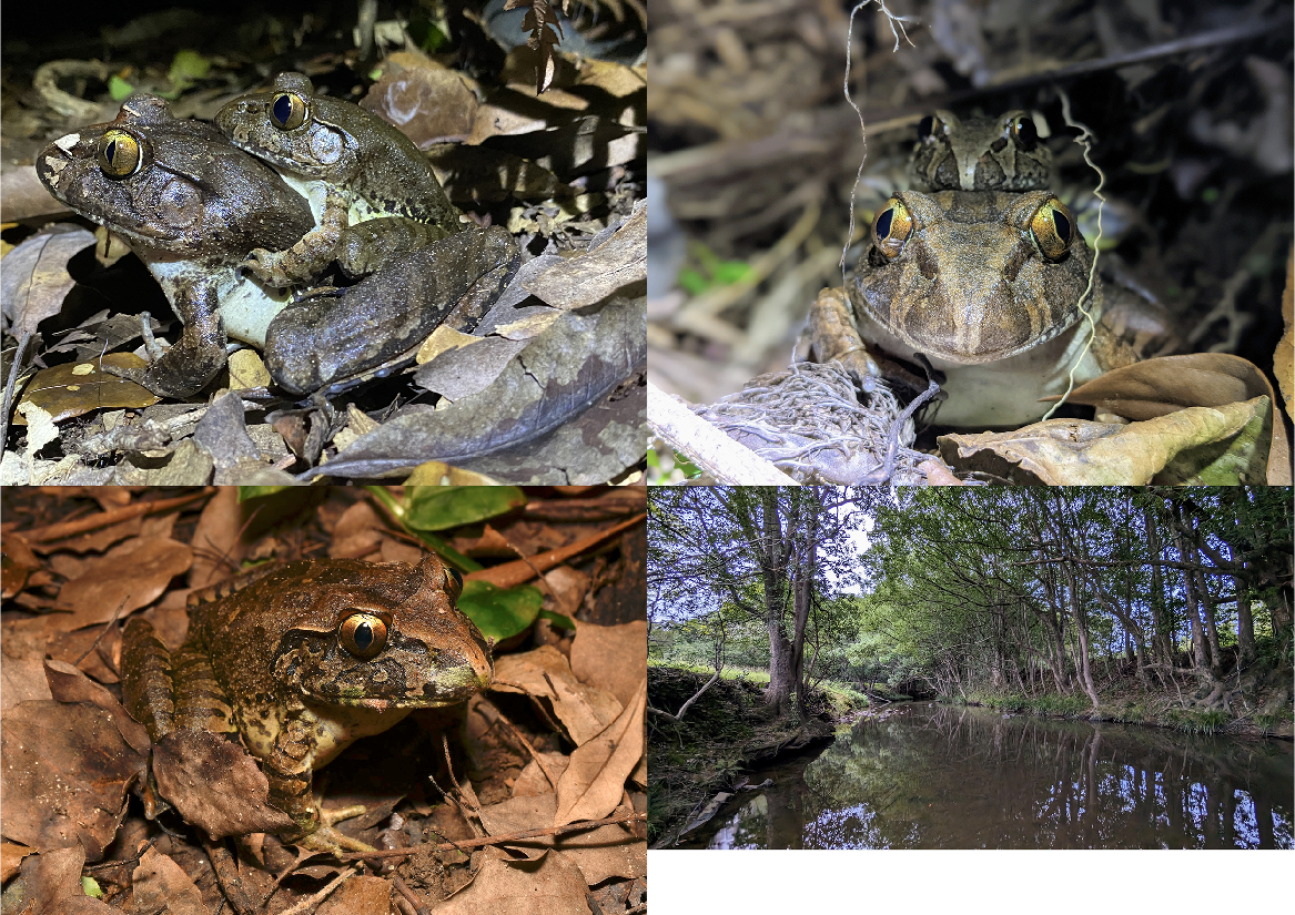
This stream-dwelling frog (Fig. 1) is known to select small scale habitat features (Lewis and Rohweder 2005) including stream areas with flat banks that are undercut at the water edge with slow flowing stream pools (Lollback et al. 2021). Riparian vegetation is often either wet sclerophyll forest or rainforest (Meyer et al. 2001). Since tadpole development takes at least 9 months to complete, the species requires permanent streams (Anstis 2013), once metamorphosed, the species will disperse, forage, find shelter and undergo mate selection on land. Due to the dependency of land, landscape scale factors may influence the presence of the species.
All frog surveys were restricted to the Tweed Valley, located in north-east New South Wales, Australia. The valley is part of an ‘erosion caldera’ that is derived from the Wollumbin Volcanic complex, which was active approximately 23 million years ago. Erosion of this volcanic complex has left escarpment and hills that enclose much of the valley from three sides, while the Pacific Ocean hems in the eastern extent. The Tweed Valley is approximately 1319.7 km2 and is subtropical, with a mean minimum and maximum temperature of 14.5°C and 25.8°C, respectively. Mean yearly rainfall is 1574.4 mm (www.bom.gov.au).
Woody vegetation cover in the Tweed Valley is approximately 56% and is comprised mostly of wet sclerophyll forest and rainforest (based upon State Government of NSW and Department of Planning and Environment 2022). Camphor laurel (Cinnamomum camphora) is an invasive weed that was introduced after the expansion of dairy farming in the Tweed during the late 1800s and early 1900s (Stubbs 2012). It is now a naturalised canopy tree within the Tweed Valley, often coexisting with a rainforest understorey.
Surveys
Nocturnal surveys were conducted by walking transects; each considered an independent site separated by at least 500 m for the purpose of achieving statistical independence. Since M. iteratus burrow under leaf litter during the non-breeding season and their tadpoles take at least 9 months to develop, transects were selected in areas with woody riparian vegetation and along permanent freshwater streams that were second order or greater, as defined by the Strahler system. Land tenure of sites varied between private ownership, conservation purpose (New South Wales government) and Tweed Shire Council land. Sites were surveyed over three consecutive breeding seasons, from October to April and repeat visits only occurred at sites within the same breeding season. Sites surveyed during the 2019/2020 breeding season were chosen for the purpose of studying microhabitat selection of M. iteratus (Lollback et al. 2021). Hence, there is a bias towards sites where M. iteratus were known to occur. Sites surveyed in following seasons were chosen to fill in gaps within the landscape and ensure there was adequate coverage across the valley. Tidal streams were not surveyed because they would not support a M. iteratus population.
Transect surveys followed the methodology for primary transects mentioned in Lollback et al. (2021). During the 2019/2020 survey season, sites were visited either once or three times. Occupancy analysis of the 2019/2020 data suggested two repeat surveys were adequate; therefore, sites surveyed during the subsequent breeding seasons were surveyed twice. Time between site visits was at least 2 weeks and maximised in the latter two seasons. That is, usually the complete suite of sites was visited once before being revisited.
Abiotic conditions were measured for the purpose of modelling detectability. Conditions were measured at the commencement and completion of each survey and averaged for the occupancy analysis. A Kestrel 3500 Weather Meter was used to measure air temperature (°C), relative humidity (%), and barometric pressure (hPa). Cloud cover (%), current rain occurrence, and occurrence of rainfall within the previous 24-h period were also recorded during the survey. The amount of rain in the previous 24 h (mm) was taken from the Bray Park weather station in Murwillumbah (www.bom.gov.au). Moon availability, the percentage of moon shining, and moon phase (%) were recorded. Transect length was also used as a covariate to model detectability.
Explanatory landscape variables used to model occupancy and maximum frog count were generated using QGIS software (QGIS Development Team 2023). The variables chosen were ones often used in scientific literature to demonstrate a relationship with frog presence or abundance. Explanatory variables chosen for analyses include cover of vegetation types (camphor laurel, rainforest, all woody vegetation), patch size, the proportion of road, stream sinuosity, stream gradient, stream order (Strahler system), proximity to national park (conservation area), elevation (AHD m), northing and easting position. An explanation on the chosen variables used in the analysis is in the Supplementary Material file S1. All landscape variables were measured from where M. iteratus presence was found to be most dense or in the case where no frogs were found, at the centre of a transect. There was only one replicate point at each transect.
To investigate the effect of scale (Jackson and Fahrig 2012; Moraga et al. 2019), vegetation explanatory variables were measured at different circular scales and linear scales around the site. Circular scales have previously been used to investigate the role of landscape in influencing amphibian species (Pope et al. 2000; Ficetola et al. 2011; Moraga et al. 2019; Green et al. 2021) and it has been suggested that isolation measures that are sampled using circular scales are better than directly measuring distance to a feature (e.g. the proportion of patch versus linear distance to next patch) (Vos and Stumpel 1996). However, the authors have noticed that M. iteratus was often found close to the stream (see Results) and likely had inadvertently travelled within the waterway (e.g. due to localised flooding) or stream riparian zone when dispersing or looking to mate. Hence, if landscape factors play a role in occurrence or abundance, the impact likely occurred in linear buffers along the stream. Circular scales were used to explore scale of effect with radii of 100 m, 200 m, 400 m, 800 m, 1600 m, and 3200 m. Stream buffers were 40 m wide (20 m each side of the stream), which coincides with survey width and 100 m wide (50 m each side of the stream). Stream buffer lengths were 100 m, 200 m, 400 m, 800 m, 1600 m, 3200 m, and 6400 m.
Analysis
Two response variables were used to investigate the relationship between M. iteratus and the landscape: (1) occurrence (presence/absence); and (2) the maximum count of frogs during a survey at each site. It has been shown that the ‘scale of effect’ (Jackson and Fahrig 2012), which is a landscape variable that has its strongest effect on a response variable, may be different for these response variables, with abundance being affected at smaller scales than occupancy (Moraga et al. 2019). Occurrence was first modelled against landscape variables using different landscape buffers at different scales with a single season model explained by MacKenzie et al. (2002). The buffer type and scale that had the lowest quasi-Akaike’s information criterion (QAIC) value (see below for further explanation of model choice) was then chosen for analysis of that particular variable. Any patterns in model performance over different scales were noted. Fit was also visually assessed at this stage and by using Pearson’s chi-squared test and estimates of parameters in relation to their variance.
Due to differing lengths of transects, the maximum count of frogs was standardised to the number of frogs per 100 m of transect and was used to compare different landscape buffers at different scales in the same manner as occurrence. However, standardised frog count was modelled against landscape variables using general additive models (GAMs) and the amount of deviance explained (which is analogous to a R-squared value in linear regression) was used for model selection. GAMs were applied to investigate the possibility of a non-linear relationship between standardised frog count and the landscape variables (Wood 2017). The Tweedie, negative binomial and quasi-Poisson response distributions and general model fit were assessed using standard GAM diagnostics. Over-fitting was assessed by plotting the fitted model with residuals and over-fitted models were rerun with a less complex degree of smoothness. Variance from each GAM was estimated using a Bayesian approach.
An information-theoretic approach was used in modelling (Burnham and Anderson 2002). All models for each analysis were selected a priori and were based on previous experience and literature (see above for justification of predictor variables chosen). That is, data mining, stepwise regression or ensemble modelling were not used in the model selection process.
After the scale-of-effect analyses was completed, correlated landscape variables (ρ ≥ 0.7, P-value <0.05) were excluded from further analyses using a Spearman’s rank correlation. The final model selection process using occupancy modelling and GAMs was then completed.
Due to data dispersion, QAIC was used when selecting occurrence models (Burnham and Anderson 2002). The over-dispersion parameter value was chosen from the global model. Models with an QAIC difference (Δi) ≤ 2 indicate significant support that it is the best suited model within the suite. Models with Δi ranging between four and seven are less supported and models with Δi > 10 are not competitive and thus omitted. The Akaike weight (wi) was also calculated. All occupancy analysis was completed in Program Presence 2.13.18 (Hines 2006).
The statistical program R ver. 4.1.2 (R Core Team 2021) was used with the package mgcv (Wood 2017) to perform the GAM analysis.
Results
There was a total of 40 transects sampled, with an average length of 726.6 m (s.d. = 334.3 m) and a minimum and maximum length of 200 and 1580 m, respectively. Thirteen transects were surveyed three times, 25 transects were surveyed twice, and three transects were surveyed once. A total of 15 transects were surveyed within the 2019/2020 breeding season, which provided data for (Lollback et al. 2021). A further 11 transects were surveyed within the 2020/2021 breeding season, and 14 other transects were surveyed during the 2021/2022 breeding season.
Surveys were conducted over a range of abiotic conditions during the breeding season. Average ambient temperature during surveys was 22.6°C (min = 15.8°C, max. = 27.3°C), average relative humidity was 92.1% (min. = 71.7%, max. = 100%), and average rainfall in the previous 24 h was 4.5 mm (min. = 0 mm, max. = 45.8 mm). It rained during 30 out of 90 surveys and it rained 44 times in the 24-h period before surveys were conducted. Average cloud cover was 46.6% (min. = 0%, max. = 100%), average moon availability was 17.5% (min. = 0%, max. = 100%), average moon phase was 48.5% (min. = 0%, max. = 100%), and average air pressure was 1055.3 hPa (min. = 979.3 hPa, max. = 1055.3 hPa).
Site (transect) location was spread across the Tweed Shire; however, there were more sites in the western half of the Shire due to the prevalence of cane farms and brackish streams closer to the coast. Site elevation varied from 1 m to 272 m (mean = 87 m), with 12 sites in national park and the average distance from national parks was 3.7 km. There were four sites located on second order reaches, 14 sites on third order reaches, 16 sites on fourth order reaches and six sites on fifth order stream reaches.
Mixophyes iteratus was detected at 21 of the 40 transects, during 45 out of the 90 surveys. During these surveys, there were 158 adults and 80 juveniles/sub-adults detected. The average number of M. iteratus found at occupied sites during a survey was 1.12 frogs per 100 m (min. = 0.12 frogs per 100 m, max. = 8.5 frogs per 100 m). The average distance a frog was found from the stream edge was 3.2 m (s.d. = 2.7 m, n = 145), with a minimum and maximum distance of 0.0 m and 15 m, respectively. In the 2019/2020 breeding season, M. iteratus was found on 73.3% of transects, while M. iteratus was detected on 45.4% and 35.7% of transects in the 2020/2021 and 2021/2022 seasons, respectively. Spatially, M. iteratus was found more often in the western half of the Tweed Shire. Frogs were found from 26 m to 203 m in elevation and across all orders of stream surveyed. A total of 70% of national park sites were occupied, while 46% of sites outside national park were occupied. Average frog count was 0.35 (0.64 s.d.) frogs per 100 m in transects outside national park, and 1.56 (2.55 s.d.) frogs per 100 m in transects inside national parks.
Occupancy analysis – scale of effect
The scale of effect where the landscape variable had its strongest effect on occurrence, was investigated before a final suite of occupancy models were analysed. The scale of effect differed between buffer types across vegetation types is in Fig. 2. For vegetation categories, the scale that consistently had the lowest QAIC values was 3200 m for either linear stream buffer or circular buffer. The relationship between scale and QAIC differed with vegetation type but was similar for the proportion of native vegetation and the proportion of total vegetation because these two variables were correlated. This was also the case with the two linear buffers.
Scale of effect graphs for landscape variables and M. iteratus occupancy, including the proportion of camphor laurel, proportion of rainforest, proportion of native vegetation, proportion of all vegetation, proportion of road, slope of stream and stream sinuosity. The x-axis is distance of stream or radius of circle (m). The y-axis is QAIC value.
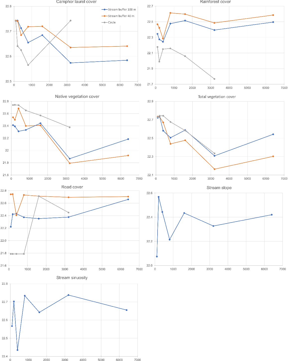
The relationship between occurrence and non-vegetation variables was different to that between occurrence and vegetation variables. The scale of effect for the proportion of road, stream slope and stream sinuosity occurred at short distances, often less than 800 m of circle radius or stream length. It is important to note that the QAIC difference between scales and buffer types for each variable was less than two, suggesting differences were minimal.
Final suite of occupancy models
Before the final suite of models were compared, a correlation matrix containing all landscape variables was assessed. Correlated variables included: the number of upstream stream heads and stream order (ρ = 0.76, P = 0.00) and longest distance to stream head (ρ = 0.81, P = 0.00); stream distance to a national park and the occurrence within a national park (ρ = −0.81, P = 0.00); connection to Gondwana forest and longitude (ρ = −0.84, P = 0.00).
After correlated variables were removed, only variables that showed the scale of effect were chosen and poor fitting models (s.e. of model coefficients twice as large as the coefficient) were removed, the final suite of models was reduced to 25 (see Table 1). Twenty models in the suite had a QAIC Δi < 2. The top performing model with the lowest QAIC modelled occupancy and detection as constant across sites and surveys. The estimates of occupancy and detection for the top performing model were 0.54 (0.08 s.e.) and 0.85 (0.06), respectively. These estimates have reasonable coefficients of variation, which gives confidence in the model.
| Model | QAIC | ΔQAIC | AIC weight | Parameter number | |
|---|---|---|---|---|---|
| ψ(.) p(.) | 20.74 | 0.00 | 0.09 | 2 | |
| ψ(Roads c_200) p(.) | 21.36 | 0.62 | 0.07 | 3 | |
| ψ(S dist to stream head) p(.) | 21.73 | 0.99 | 0.05 | 3 | |
| ψ(RF c_3200 RF) p(.) | 21.77 | 1.02 | 0.05 | 3 | |
| ψ(Nat veg 40_3200) p(.) | 21.79 | 1.05 | 0.05 | 3 | |
| ψ(Tot veg 40_3200) p(.) | 22.16 | 1.42 | 0.04 | 3 | |
| ψ(Dist NP) p(.) | 22.17 | 1.43 | 0.04 | 3 | |
| ψ(RF 100_40) p(.) | 22.24 | 1.50 | 0.04 | 3 | |
| ψ(Tot veg c_3200) p(.) | 22.33 | 1.59 | 0.04 | 3 | |
| ψ(Slope 100) p(.) | 22.42 | 1.68 | 0.04 | 3 | |
| ψ(X) p(.) | 22.42 | 1.68 | 0.04 | 3 | |
| ψ(Sinuosity) p(.) | 22.44 | 1.70 | 0.04 | 3 | |
| ψ(.) p(Temp) | 22.46 | 1.72 | 0.04 | 3 | |
| ψ(.) p(Pressure) | 22.47 | 1.73 | 0.04 | 3 | |
| ψ(Join NP) p(.) | 22.49 | 1.74 | 0.04 | 3 | |
| ψ(AHD) p(.) | 22.57 | 1.82 | 0.04 | 3 | |
| ψ(Camphor 100_3200 p(.) | 22.57 | 1.83 | 0.04 | 3 | |
| ψ(.) p(Cloud cover) | 22.65 | 1.90 | 0.03 | 3 | |
| ψ(.) p(Raining) | 22.68 | 1.94 | 0.03 | 3 | |
| ψ(.) p(Moon av) | 22.70 | 1.95 | 0.03 | 3 | |
| ψ(Y) p(.) | 22.80 | 2.06 | 0.03 | 3 | |
| ψ(Road c_3200) p(Pressure) | 23.10 | 2.36 | 0.03 | 4 | |
| ψ(Dist NP + Tot Veg 40_3200) p(.) | 23.71 | 2.97 | 0.02 | 4 | |
| ψ(Slope + Sinuosity) p(.) | 23.99 | 3.25 | 0.02 | 4 | |
| ψ(.) p(Temp + Humidity) | 24.06 | 3.32 | 0.02 | 4 |
QIAC, quasi-Akaike’s information criterion; ψ, occupancy; p, detection rate, and ‘. ’ is when occupancy or detection rate was held constant. Landscape variables include density of road (‘Roads’), distance to stream head (‘S dist to stream head’), proportion of rainforest (‘RF’), proportion of native vegetation (‘Nat veg’), proportion of total woody vegetation (‘Tot veg’), distance to conservation area (‘Dist NP’), stream gradient (‘Slope’), longitude (X), stream sinuosity (‘Sinuosity’), if the site was within a conservation area (‘Join NP’), elevation (‘AHD’), proportion of camphor laurel (‘Camphor’), latitude (‘Y’) and road cover (‘Road’). Numbers within model names indicate either circle (‘c’) radius or stream buffer width and then length. Variables used to model detection rate and included in the table are ambient temperature (‘Temp’), barometric pressure (‘Pressure’), cloud cover (‘Cloud cover’), if it was raining during the survey (‘Raining’), moon availability (‘Moon av’) and humidity percentage (‘Humidity’).
GAM analysis
The visual investigation of diagnostic charts for various GAMs suggested that quasi-Poisson models fitted the data better than models that used a negative binomial or Tweedie response distribution. Hence, all model selections that used standardised maximum frog count as a response variable were quasi-Poisson models.
GAM analysis – scale of effect
The scale of effect when using standardised maximum frog count occurred at various scales, depending on the landscape variable (Fig. 3). The scale of effect for the proportion of camphor and the proportion of all vegetation, the proportion of road and sinuosity was 3200 m radius/distance of stream. Out of five variables, circular scales performed better than stream buffers. There were no linear response variables that continually decreased or increased along scale.
Scale of effect graphs for landscape variables and M. iteratus maximum count, including the proportion of camphor laurel cover, proportion of rainforest cover, proportion of native vegetation cover, proportion of all vegetation cover, proportion of road cover, and slope of stream is stream sinuosity. The x-axis is distance of stream or radius of circle (m). The y-axis is percentage deviance explained.

Final suite of frog count models
As well as the previously mentioned occupancy analysis variables that correlated, the proportion of road within a 3200-m radius circle correlated with the proportion of native vegetation in a 1600-m radius circle (ρ = −0.85, P = 0.00), the proportion of total vegetation within a 3200-m radius circle (ρ = −0.89, P = 0.00) and the number of upstream stream heads (ρ = 0.72, P = 0.00). Correlated variables were removed from the suite of models.
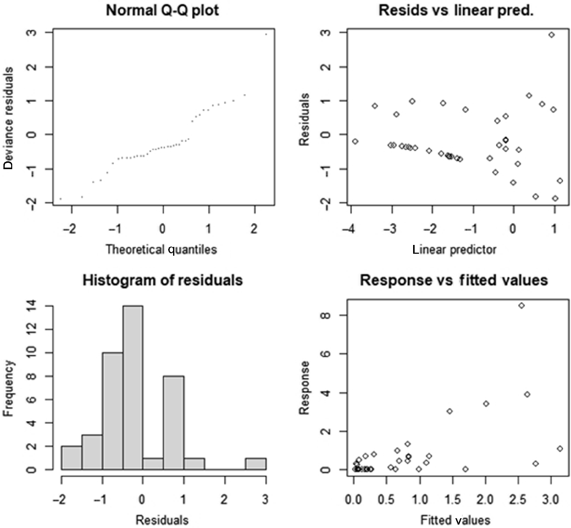
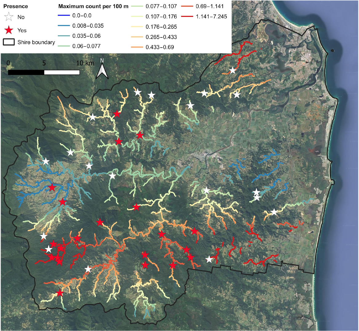
The top performing model explained frog counts with an interaction between longitude and latitude, suggesting some spatial clumping in counts across the Shire (Table 2). The model fit is in Fig. 4. The top six models were reasonably close in performance and four of these models used longitude and/or latitude to explain frog counts. Other top performing models had either the shortest distance to a stream head or the proportion of road within a circle with a radius of 3200 m (Fig. 5). As with the occupancy analysis, other landscape scale variables were poor predictors of the number of frogs counted per 100 m of transect. The top model was used to model frog count across the Tweed Valley (Fig. 6). Modelling mirrored counts in the south-western and southern part of the Tweed Valley but was likely a poor predictor of density in the northeast.
| Model | Deviance explained by model (%) | |
|---|---|---|
| X*Y (te) | 54.7 | |
| Shortest distance to stream head | 47.5 | |
| X + Y | 45.3 | |
| Road c_3200 | 44.4 | |
| Y | 40.1 | |
| X | 40.1 | |
| AHD | 28.1 | |
| Camphor c_3200 | 25.5 | |
| Slope 200 | 20.5 | |
| Sinuosity 3200 | 18.2 | |
| stream order | 17.6 | |
| RF 100_400 | 17.3 | |
| Distance to NP | 15.8 | |
| Longest distance to stream head | 13.1 | |
| Join NP | 3.04 |
*, interaction term; te, full tensor product smoothing was used when modelling the GAM. Models are ranked by the percentage of deviance explained. Variables used to model maximum frog count and shown in the table below include longitude (‘X’), latitude (‘Y’), shortest distance to stream head, road cover within a circle that has a radius of 3200 m, elevation (‘AHD’), camphor laurel cover within a circle with a radius of 3200 m, (‘Camphor c_3200’), stream gradient over a distance of 200 m (‘Slope 200’), stream sinuosity over a distance of 3200 m (‘Sinuosity 3200’), stream order, rainforest cover within a 100 m stream buffer for a length of 400 m (‘RF 100_400’), distance to a conservation area (‘Distance to NP’), longest distance to stream head and whether a site was within a conservation area (‘Join NP’).
The best performing GAM model, maximum count = X*Y, showing residuals and diagnostic information.
The second and fourth best performing GAM models showing residuals and diagnostic information. (a) GAM with the proportion of road within a circle that has a radius of 3200 m, (b) GAM with the shortest distance to an upstream stream head, (c) diagnostic plots for (a), and (d) diagnostic plots for (b). The triangles in (a) and (b) are residuals and the dashed lines are 95% confidence intervals.

Discussion
This study looked at the distribution of M. iteratus throughout the Tweed Valley landscape at 40 transect sites with differing elevations, proportions of vegetation cover, stream morphology types and distance to conservation reserves. The vulnerable M. iteratus was detected at 21 of these sites. Previous surveys of the species within the Tweed Valley have been limited (Goldingay et al. 1999), resulting in much uncertainty regarding its distribution within the study area. While the vulnerable status of the species is justified, the species is much more broadly distributed across the Tweed Valley than previously thought. Goldingay et al. (1999) found M. iteratus occupied sites less than 300 m in elevation. All survey sites used during this study were located less than 300 m in elevation and stream reaches above this elevation are likely to be first order gullies that are too steep and rocky and lack permanent water to provide quality habitat for the species. While according to the analyses there was no distinguishing association between M. iteratus occupancy or counts and national parks, there does seem to be a mildly favourable association in abundance/occupancy and national parks. National parks in the Tweed Valley are generally exempt from ongoing vegetation clearing and can contain more mature vegetation, have greater canopy cover and less disturbance than private land. These features likely create more plant litter for burrowing and foraging habitat, while providing a more stable microclimate, better water quality and habitat that is more flood resilient for M. iteratus. National parks within the Tweed Valley are often situated in steep, higher elevated land that is unfavourable for grazing or cropping. While this type of topography can also be restricting in regard to habitat availability for M. iteratus, national parks often encompass the heads of streams where M. iteratus populations have been found to occur and they may act as source populations where tadpoles and juvenile frogs become washed downstream during high flow events.
Analyses suggested that there was no strong relationship between M. iteratus occupancy and landscape features and this was reflected in only small differences in QAIC value when investigating scale of effect. Moraga et al. (2019) hypothesised that occurrence, which generally takes generations to change, should be influenced at broad scales. They also hypothesised that trends in occurrence should occur at larger scales than trends in abundance. They found that there was a scale of effect regarding wood frog (Lithobates sylvaticus) occurrence and road density; however, the relationship between occurrence and the scale of forest cover was not clear. Additionally, scale of effect for wood frog abundance did not occur at a much smaller scale than occurrence. Jackson and Fahrig (2012) reasoned that the scale of effect is less likely to exist in gap-avoidant species and although M. iteratus requires a forested riparian zone, the species likely can travel through forest gaps by using the stream to disperse. Many streams in the Tweed Valley have a continual thin section of riparian vegetation, including some occupied sections of stream (<70 m wide). Mixophyes iteratus frog count also displayed a larger scale of effect than occupancy for cover of some vegetation types, proportion of road and stream sinuosity, which dispels the hypothesis postulated by Moraga et al. (2019).
Not surprisingly, the response to large scale effects appears to be species specific (Kolozsvary and Swihart 1999; Ficetola and De Bernardi 2004), as has been the case with Australian frog species and elevation, distance to large reserves (Lemckert 1999), solar radiation, moisture level (Lemckert and Mahony 2010) and area of native canopy within 1 km radius (Hazell et al. 2001). Lemckert (1999) did find an association between occupancy of M. iteratus and percentage of undisturbed forest within 500 m. Most of the sites surveyed within the Tweed Valley had a history of disturbance, so this variable could not be tested on a large scale. However, disturbance level was investigated at a small scale in Lollback et al. (2021) and found not to be an important factor in influencing M. iteratus occupancy. Nevertheless, it was deemed an influencing factor when assessed by Lewis and Rohweder (2005). Agents and measures of disturbance, including weed prevalence, fire history, agricultural history, and erosion may influence frog occurrence and the importance of disturbance should not be dismissed. However, our study would need to have different site selection methodology to test this hypothesis suitably and would be better reflected by measuring variables at a smaller scale. Nevertheless, undisturbed sites would likely contain better tree cover, leaf litter coverage, understorey cover along banks and water quality and some disturbance may also be measured at a larger scale (e.g. land tenure). In contrast, drought is a stochastic process that often occurs over a wider scale than a single landscape and can indeed influence occupancy by causing localised extinction to species that are dependent upon waterways. This study occurred just after a drought, but included sites were surveyed more than two decades ago (Goldingay et al. 1999) and were found to be still occupied by M. iteratus (see Lollback et al. 2021 for further details).
Mixophyes iteratus appears to be robust to habitat fragmentation within the Tweed Valley may be because the species can disperse via steams, thereby avoiding ‘matrix’ type land unlike pond-breeding species where fragmentation has been shown to influence occupancy (Knapp et al. 2003; Ficetola and De Bernardi 2004; Mazerolle et al. 2005; D’Amore et al. 2010; Green et al. 2021). Many of the streams within the Tweed Valley do not display fragmentation of ‘longitudinal connectivity’ (Erős and Campbell Grant 2015) in the form of dams, flooding or extreme changes in water quality, with connectivity along the streams being maintained (Fig. 7); and many of the streams within the Tweed Valley contain a narrow corridor of vegetation, which is enough to disperse across land and provide breeding habitat. Although heavily disturbed from past clearing, weed invasion, cattle grazing, land shaping, and vegetation modification, the Tweed Valley still contains approximately 56% woody vegetation cover (taken from Office of Environment and Heritage 2012 dataset). This likely allows the distribution of M. iteratus across the Tweed Valley landscape to be broad, especially in the western and south-western sections of the Valley.
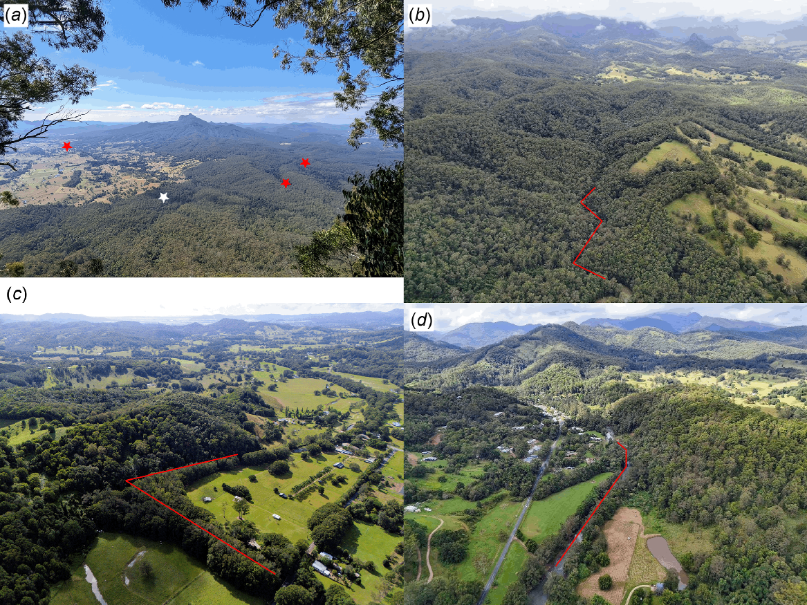
(a) Transect locations in the landscape showing view from Border Ranges National Park overlooking Mebbin National Park, the Limpinwood area and Wollumbin Red stars, locations where Mixophyes iteratus was detected; white star, location where M. iteratus was not detected. (b) View of a survey location within Doon Doon area. (c) View of a survey location within the Crystal Creek area. (d) View of a survey location within the Chillingham area. Images (b), (c) and (d) show approximate transect locations (red line) where M. iteratus were detected.
This is not the only study to indicate some landscape scale relationship with frog count. Like this study, da Silva et al. (2011) found a relationship with frog abundance and roads and Atobe et al. (2014) found a relationship with connectivity and frog count. Roads may cause isolation and increase mortality (Fahrig et al. 1995; Vos and Chardon 1998; Goldingay and Taylor 2006), but road influence would likely occur on a small scale, unlike this study where the scale of effect was at 3200 m diameter. It is more likely that sites with large counts occurred in larger forest patches with fewer roads at a large scale (for example, national parks). These forest patches tended to have better quality habitat that could support higher abundance. This may be the case even if forest cover was not a good predictor of abundance because the important factor may not be patch size, but only if the patch is small or large. Landscape features can indirectly influence species by shaping or coinciding with smaller habitat scale attributes (Ficetola et al. 2011). For example, the edges of large forest patches may offer a buffer from disturbance to core vegetation (Saunders et al. 1991) or large patches may indicate minimal historical disturbance. Either way, the result is better quality small-scale features in large patches.
The best predictor of maximum M. iteratus count was the interaction between easting (X) and northing (Y), with higher counts occurring around Mebbin National Park in the south-west of the Tweed Valley (Fig. 6). While this area was not without disturbance, stream structure, and surrounding vegetation was of generally good quality. Areas near Mount Jerusalem National Park also revealed good counts. Nevertheless, the best landscape predictor could only account for approximately 57% of count variation. This is to be expected due to the potential dynamic behaviour of abundance and the number of factors that can influence it (Krebs 1994).
Stream features within Mooball National Park appeared typical of what M. iteratus would occupy. However, like the other eastern sites of the Tweed Shire, the species was absent. It appears that while small scale factors may influence occupancy and abundance, there is also a large-scale spatial influence on the species. This influence may have initially occurred well before the arrival of Europeans and the clearing of forest and may be more aligned with distribution expansion and topographical features not measured here.
The absence of strong large-scale patterns with relative abundance and occupancy likely reflects species ecology and pre-clearing (late 1800s) distribution within the Tweed Valley. It is known that M. iteratus displays a strong selection for small-scale stream features (Lollback et al. 2021) and these features were likely more common across the Valley, including the lower elevation areas where stream velocity is slower. It is likely that M. iteratus was once a common frog species in the Tweed Valley, especially the southern and western sections, before broadscale land clearing occurred.
Implications for management
Within the Tweed Shire, this species appears robust to disturbance, excluding extensive clearing, as indicated by its broad distribution. Conservation for the species would be most effective if focused around streams that have favourable habitat features on a small scale (Lollback et al. 2021). The species was found at numerous sites where land management improvements such as cattle exclusion and the widening of the riparian zone of at least 15 m would likely bolster their numbers. Such action would consequentially increase litter cover/depth and vegetation cover, which in turn increases sheltering and foraging opportunities and potentially reduces bank collapse (thereby increasing the likelihood of undercut banks that is favourable for breeding). The distribution map produced here indicates favourable areas to focus conservation efforts where predicted counts are middle to low range in the western half of the Tweed Valley. Additionally, continual conservation of national parks would ensure future existence of the species within the Tweed Valley. Greater knowledge of the species’ distribution across a landscape (outside the study area) would aid both narrow and broad conservation efforts.
While not related to effect of scale, this study over three seasons has implications for survey design. Lollback et al. (2021) used short 100 m surveys to estimate detection rate, which was 0.54 and 0.65 after three site visits. However, this study estimated detection rate to be 0.85 using longer transect lengths (average length was 726 m). When surveying the species, it is recommended that 1 km transects in suitable habitat are used and that each transect is surveyed twice.
Acknowledgements
We Thank the two anonymous reviewers for improving the manuscript. We also thank Kathleen Hellmann and NSW National Parks and Wildlife Service for allowing the study to include sites within Mebbin National Park, Mount Jerusalem National Park, and Duroby Nature Reserve. We thank Liam Thompson, Jon Shuker, and Gemma Bauld for assisting with frog surveys. Matthew Bloor and Michael Corke provided valuable information on Mixophyes iteratus occurrences. Stuart Cairns provided philosophy, ecological knowledge, and statistical advice. We are grateful to the various landholders within the Tweed Valley that kindly let us conduct research on their land. We also thank our families for supporting this work. Fieldwork was conducted under NSW Department of Climate Change, Energy, the Environment and Water Scientific Licence SL100540.
References
Atobe T, Osada Y, Takeda H, Kuroe M, Miyashita T (2014) Habitat connectivity and resident shared predators determine the impact of invasive bullfrogs on native frogs in farm ponds. Proceedings of the Royal Society B: Biological Sciences 281, 20132621.
| Crossref | Google Scholar |
Banks B, Beebee TJC (1987) Factors influencing breeding site choice by the pioneering amphibian Bufo calamita. Ecography 10, 14-21.
| Crossref | Google Scholar |
Blomquist SM, Hunter ML, Jr. (2010) A multi-scale assessment of amphibian habitat selection: wood frog response to timber harvesting. Écoscience 17, 251-264.
| Crossref | Google Scholar |
Bosch J, Martínez-Solano I (2003) Factors influencing occupancy of breeding ponds in a montane amphibian assemblage. Journal of Herpetology 37, 410-413.
| Crossref | Google Scholar |
Brown C, Nowakowski AJ, Keung NC, Lawler SP, Todd BD (2021) Untangling multi-scale habitat relationships of an endangered frog in streams to inform reintroduction programs. Ecosphere 12, e03799.
| Crossref | Google Scholar |
da Silva FR, Gibbs JP, Rossa-Feres DDC (2011) Breeding habitat and landscape correlates of frog diversity and abundance in a tropical agricultural landscape. Wetlands 31, 1079-1087.
| Crossref | Google Scholar |
D’Amore A, Hemingway V, Wasson K (2010) Do a threatened native amphibian and its invasive congener differ in response to human alteration of the landscape? Biological Invasions 12, 145.
| Crossref | Google Scholar |
Erős T, Campbell Grant EH (2015) Unifying research on the fragmentation of terrestrial and aquatic habitats: patches, connectivity and the matrix in riverscapes. Freshwater Biology 60, 1487-1501.
| Crossref | Google Scholar |
Fahrig L, Pedlar JH, Pope SE, Taylor PD, Wegner JF (1995) Effect of road traffic on amphibian density. Biological Conservation 73, 177-182.
| Crossref | Google Scholar |
Ficetola GF, De Bernardi F (2004) Amphibians in a human-dominated landscape: the community structure is related to habitat features and isolation. Biological Conservation 119, 219-230.
| Crossref | Google Scholar |
Ficetola GF, Marziali L, Rossaro B, De Bernardi F, Padoa-Schioppa E (2011) Landscape–stream interactions and habitat conservation for amphibians. Ecological Applications 21, 1272-1282.
| Crossref | Google Scholar | PubMed |
Goldingay R, Taylor B (2006) How many frogs are killed on a road in north-east New South Wales? Australian Zoologist 33, 332-336.
| Crossref | Google Scholar |
Green J, Govindarajulu P, Higgs E (2021) Multiscale determinants of Pacific chorus frog occurrence in a developed landscape. Urban Ecosystems 24, 587-600.
| Crossref | Google Scholar | PubMed |
Hazell D (2003) Frog ecology in modified Australian landscapes: a review. Wildlife Research 30, 193-205.
| Crossref | Google Scholar |
Hazell D, Cunnningham R, Lindenmayer D, Mackey B, Osborne W (2001) Use of farm dams as frog habitat in an Australian agricultural landscape: factors affecting species richness and distribution. Biological Conservation 102, 155-169.
| Crossref | Google Scholar |
Hinderer RK, Litt AR, McCaffery M (2021) Habitat selection by a threatened desert amphibian. Ecology and Evolution 11, 536-546.
| Crossref | Google Scholar | PubMed |
Hines JE (2006) PRESENCE - Software to estimate patch occupancy and related parameters. Available at http://www.mbr-pwrc.usgs.gov/software/presence.html
Hodgkison S, Hero J-M (2001) Daily behavior and microhabitat use of the waterfall frog, Litoria nannotis in Tully Gorge, eastern Australia. Journal of Herpetology 35, 116-120.
| Crossref | Google Scholar |
Jackson HB, Fahrig L (2012) What size is a biologically relevant landscape? Landscape Ecology 27, 929-941.
| Crossref | Google Scholar |
Knapp RA, Matthews KR, Preisler HK, Jellison R (2003) Developing probabilistic models to predict amphibian site occupancy in a patchy landscape. Ecological Applications 13, 1069-1082.
| Crossref | Google Scholar |
Kolozsvary MB, Swihart RK (1999) Habitat fragmentation and the distribution of amphibians: patch and landscape correlates in farmland. Canadian Journal of Zoology 77, 1288-1299.
| Crossref | Google Scholar |
Lehtinen RM, Carfagno GLF (2011) Habitat selection, the included niche, and coexistence in plant-specialist frogs from Madagascar. Biotropica 43, 58-67.
| Crossref | Google Scholar |
Lemckert F (1999) Impacts of selective logging on frogs in a forested area of northern New South Wales. Biological Conservation 89, 321-328.
| Crossref | Google Scholar |
Lemckert F, Mahony M (2010) The relationship among multiple-scale habitat variables and pond use by Anurans in northern New South Wales, Australia. Herpetological Conservation and Biology 5, 537-547.
| Google Scholar |
Lewis BD, Rohweder DA (2005) Distribution, habitat, and conservation status of the giant barred frog Mixophyes iteratus in the Bungawalbin catchment, northeastern New South Wales. Pacific Conservation Biology 11, 189-197.
| Crossref | Google Scholar |
Lollback GW, Lockwood MA, Hannah DS (2021) New information on site occupancy and detection rate of Mixophyes iteratus and implications for management. Pacific Conservation Biology 27, 244.
| Crossref | Google Scholar |
MacKenzie DI, Nichols JD, Lachman GB, Droege S, Royle JA, Langtimm CA (2002) Estimating site occupancy rates when detection probabilities are less than one. Ecology 83, 2248-2255.
| Crossref | Google Scholar |
Mayor SJ, Schneider DC, Schaefer JA, Mahoney SP (2009) Habitat selection at multiple scales. Écoscience 16, 238-247.
| Crossref | Google Scholar |
Mazerolle MJ, Desrochers A, Rochefort L (2005) Landscape characteristics influence pond occupancy by frogs after accounting for detectability. Ecological Applications 15, 824-834.
| Crossref | Google Scholar |
McEwan AL, Johnson CJ, Todd M, Govindarajulu P (2021) Resource selection and movement of the coastal tailed frog in response to forest harvesting. Forest Ecology and Management 497, 119448.
| Crossref | Google Scholar |
Moraga AD, Martin AE, Fahrig L (2019) The scale of effect of landscape context varies with the species’ response variable measured. Landscape Ecology 34, 703-715.
| Crossref | Google Scholar |
Office of Environment and Heritage (2012) Tweed LGA Vegetation 2012. VIS_ID 3912. Available at https://datasets.seed.nsw.gov.au/dataset/tweed-lga-vegetation-2012-vis_id-3912e0407
Pizzatto L, Stockwell M, Clulow S, Clulow J, Mahony M (2016) Finding a place to live: conspecific attraction affects habitat selection in juvenile green and golden bell frogs. Acta Ethologica 19, 1-8.
| Crossref | Google Scholar |
Pope SE, Fahrig L, Merriam HG (2000) Landscape complementation and metapopulation effects on leopard frog populations. Ecology 81, 2498-2508.
| Crossref | Google Scholar |
Pulsford SA, Lindenmayer DB, Driscoll DA (2017) Reptiles and frogs conform to multiple conceptual landscape models in an agricultural landscape. Diversity and Distributions 23, 1408-1422.
| Crossref | Google Scholar |
QGIS Development Team (2023) QGIS Geographic Information System. Available at https://www.qgis.org
R Core Team (2021) R: A language and environment for statistical computing. Available at https://www.R-project.org/
Saunders DA, Hobbs RJ, Margules CR (1991) Biological consequences of ecosystem fragmentation: a review. Conservation Biology 5, 18-32.
| Crossref | Google Scholar |
Shuker JD, Hero J-M (2012) Perch substrate use by the threatened wallum sedge frog (Litoria olongburensis) in wetland habitats of mainland eastern Australia. Australian Journal of Zoology 60, 219-224.
| Crossref | Google Scholar |
Simpkins CA, Shuker JD, Lollback GW, Castley JG, Hero JM (2014) Environmental variables associated with the distribution and occupancy of habitat specialist tadpoles in naturally acidic, oligotrophic waterbodies. Austral Ecology 39, 95-105.
| Crossref | Google Scholar |
State Government of NSW and Department of Planning and Environment (2022) NSW state vegetation type map, accessed from The Sharing and Enabling Environmental Data Portal. Available at https://datasets.seed.nsw.gov.au/dataset/95437fbd-2ef7-44df-8579-d7a64402d42d [Accessed 8 November 2023]
Straughan IR (1968) A taxonomic review of the genus Mixophyes (Anura, Leptodactylidae). Proceedings of the Linnean Society of New South Wales 93, 52-59.
| Google Scholar |
Stubbs BJ (2012) Saviour to scourge: a history of the introduction and spread of the camphor tree (Cinnamomum camphora) in eastern Australia. In ‘Australia’s Ever-changing Forests VI: Proceedings of the Eighth National Conference on Australian Forest History’. Australian Forest History Series. (Eds BJ Stubbs, J Lennon, A Specht, J Taylor). (Australian Forest History Society Inc.: Canberra, Australia)
Van Buskirk J, Smith DC (2021) Ecological causes of fluctuating natural selection on habitat choice in an amphibian. Evolution 75, 1862-1877.
| Crossref | Google Scholar | PubMed |
Vos CC, Chardon JP (1998) Effects of habitat fragmentation and road density on the distribution pattern of the moor frog Rana arvalis. Journal of Applied Ecology 35, 44-56.
| Crossref | Google Scholar |
Vos CC, Stumpel AHP (1996) Comparison of habitat-isolation parameters in relation to fragmented distribution patterns in the tree frog (Hyla arborea). Landscape Ecology 11, 203-214.
| Crossref | Google Scholar |