
Habitat suitability modelling of the North Flinders Ranges thick-billed grasswren Amytornis modestus raglessi reveals dynamic shifts at the landscape scale
David L. Gobbett A , Andrew B. Black B and Alex J. Nankivell A C *
A
B
C
Abstract
The threatened subspecies of thick-billed grasswren, Amytornis modestus raglessi, occupies dense chenopod shrublands on the lower slopes and peripheral drainages of the North Flinders Ranges, South Australia. A decline in grasswren numbers was observed around 2012, after two preceding years of exceptionally high rainfall. Profound reduction in observed numbers was also evident in 2019, the second successive year of exceptionally hot and dry conditions, in areas where they had previously been numerous.
To identify environmental factors influencing A. m. raglessi habitat suitability using habitat suitability modelling, and to better understand possible drivers of grasswren decline and distributional changes between pre- and post-2012 periods.
Random forest modelling was used to predict grasswren habitat suitability in response to mapped environmental variables including remotely sensed vegetation, soil and landscape properties. Habitat suitability maps were produced for two separate periods, 1994–2011 and 2012–2023, and compared. An ornithological field survey was undertaken to validate the modelling, and vegetation time-series used to examine areas showing contrasting habitat suitability changes.
Mapped soil properties and the minimum green vegetation cover value were the most important habitat suitability predictors. The overall predicted area of habitat (suitability >50%) declined by 25% between the 1994–2011 and 2012–2023 periods. Changes included an expansion of high-suitability habitat in the west, and habitat contraction in south-eastern areas of the distribution. Time-series vegetation data showed that lower bare ground cover and higher non-green vegetation cover occurred in an area with marked reduction in predicted habitat suitability.
Habitat suitability modelling successfully identified key environmental drivers and demonstrated habitat shifts between periods. Soil properties and minimum green vegetation cover confirmed that water stress responses are fundamental to grasswren distribution. Modelling identified areas of habitat contraction that highlight conservation priorities, while also demonstrating management effectiveness in improving habitat quality.
These methods provide spatially explicit guidance for prioritizing conservation efforts for this subspecies and thick-billed grasswrens broadly. Demonstrated habitat improvement following reduced grazing at Witchelina illustrates the practical value of this modeling approach. Such methods are increasingly essential for land managers to understand biodiversity responses and species distributions under climate change.
Keywords: Amytornis modestus raglessi, arid landscapes, chenopod, climate, conservation management, Flinders Ranges, habitat change, habitat suitability model, random forest, thick-billed grasswren, threatened species.
Introduction
Within the family Maluridae, the arid-adapted grasswrens genus Amytornis have the highest proportion of threatened species and the only extinct taxa (Skroblin and Murphy 2013). Of 13 presently recognised species (Black and Gower 2017; Black et al. 2020), the thick-billed grasswren Amytornis modestus includes five largely disjunct, extant subspecies, distributed between northern South Australia and north-western New South Wales, and two extinct subspecies, from Central Australia and eastern New South Wales (Black 2011, 2016). All surviving subspecies are threatened with extinction, three judged to be Vulnerable and two Endangered, one critically (Garnett and Baker 2021). The subspecies A. m. raglessi occupies the lower slopes and peripheral drainages of the North Flinders Ranges, South Australia. Many early records identified Mount Lyndhurst Station as its centre of distribution, and field research showed the subspecies’ dependence on dense chenopod shrublands dominated by blackbush Maireana pyramidata and low bluebush M. astrotricha, less frequently cottonbush M. aphylla and spiny saltbush Rhagodia spinescens (Pedler et al. 2007; Black et al. 2011). The subspecies is listed as Vulnerable under the Commonwealth Environment Protection and Biodiversity Protection Act (Black et al. 2021).
It is difficult to ascertain how thick-billed grasswrens are faring across their distribution, and survey efforts have not been uniform. Thick-billed grasswrens were known to occur on Witchelina Station (Badman 1981) and in 2010, Nature Foundation (as Nature Foundation SA) purchased the former sheep pastoral property, a holding of over 4000 km2, with the aim of enhancing arid zone biodiversity conservation. Surveys by Birds SA volunteers during 2010 and 2011 and a transect survey in December 2011 demonstrated an especially high density of grasswrens in the reserve (Nankivell and Black 2021). The Birds SA surveys have been repeated yearly (apart from 2017) and now form a relatively consistent dataset of the subspecies but are limited to the Witchelina reserve itself. Three more geographically extensive but time restricted surveys (Pedler et al. 2007; Black et al. 2011; G. Carpenter, M. Louter, K. Jones, D. Hopton, S. Gordon, A. Slender, unpubl. data) have been undertaken in 2007, 2007–2008 and 2021 respectively.
From anecdotal and published reports, overall numbers of grasswren have exhibited substantial variability over the years of available data. After the large numbers of grasswrens documented by Birds SA on Witchelina during 2010 and 2011, years of exceptionally high rainfall, a decline became evident as early as the following year (AB, P Waanders and M. Louter personal observations, Black and Gower 2017). There was some apparent recovery by 2016 but a further and more severe deterioration was suspected following the record dry and hot years of 2018 and 2019 (Nankivell and Black 2021). When the December 2011 transect survey was repeated in September 2019, only two grasswrens were observed compared with 107 individuals 8 years earlier. A comparable collapse of the grasswren population was also evident at Mount Lyndhurst Station in March 2020; two grasswrens were seen at only one of the 23 known grasswren presence sites and one was recorded opportunistically (AB and K Jones unpubl. data). Birdata (Birdlife Australia 2025) includes a total of 170 surveys in which thick-billed grasswrens were reported since 1998 within the area shown in Fig. 1, with a mean reporting rate of 4.2% and a peak rate of 11.5% in 2008, but only 3.0% since 2012.
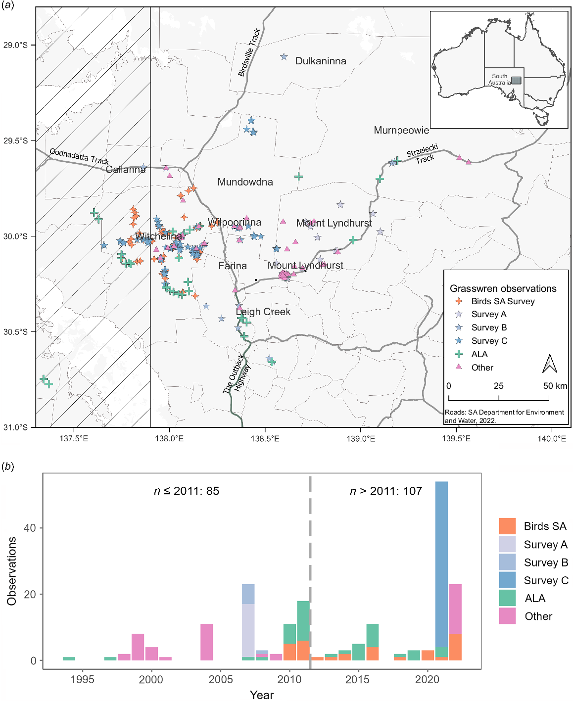
(a) Map of the study area showing locations of Amytornis modestus raglessi observations from 1994 to 2023 (see text for a description of the sources of observations). The hatched section is the designated zone of hybridisation with A. m. indulkanna, from which observations were excluded for modelling (b) plot showing the numbers of cleaned observations over the same period. Surveys A, B and C being surveys by Pedler et al. (2007), Black et al. (2011) and G. Carpenter et al. unpubl. data respectively. ALA observations are sourced from Atlas of Living Australia (2023).
A survey of grasswrens on Witchelina and adjacent properties Mundowdna, Wilpoorinna and Mount Lyndhurst Stations in April–May and August–September of 2021 (G. Carpenter et al. unpubl. data) showed that decline in the grasswrens numbers on Witchelina was far less severe than had been inferred from earlier observations, with little if any evidence of reduced territory occupation. However, the loss of grasswrens from Mount Lyndhurst Station, a former stronghold for the subspecies, appeared confirmed and profound. On Mundowdna and Wilpoorinna, grasswrens were present in possibly reduced numbers but comparison with earlier periods was less clear because of fewer data. Of the 170 Birdata surveys mentioned above, 95 (56%) were from a small area of approximately 10 km2 on Mount Lyndhurst Station close to the Strzelecki Track; 87 records occurred prior to 2012 and there have been only eight sightings since.
Clearly there is a high degree of temporal variability in the records of this cryptic grasswren because of the vagaries of climate and land management practices, and its likely variable detectability under different conditions and survey methods (Nankivell and Black 2021). Understanding this variability is challenging and an improved understanding of changes in the distribution of suitable habitat is needed.
Habitat suitability modelling (HSM) is the process of using environmental data and statistical modelling methods to predict the potential distribution of suitable habitat for species across a landscape (e.g. Thuiller and Münkemüller 2010; Bradley et al. 2012). HSM is conceptually and methodologically similar to species distribution models (SDM) and ecological niche models (ENM) (Hirzel and Le Lay 2008). A species may not always occupy the full extent of suitable habitat due to poor connectivity (restricting dispersal), or the effects of disturbance (Brown and Griscom 2022) which may take the form of climatic extremes or anthropogenic impacts, so HSM only predicts the geographic area that might be suitable to the species, not the area occupied (Thuiller and Münkemüller 2010). Such modelling is frequently carried out with presence-only observation data, and utilising modelling methods such as random forest (e.g. Thuiller and Münkemüller 2010; Hijmans and Elith 2021; Valavi et al. 2021).
In this modelling study, we utilised HSM to understand vegetation, soil and landscape factors influencing the distribution of A. m. raglessi. By generating and comparing predicted distributions for the periods before and after the exceptionally high rainfall years of 2010 and 2011, we identified factors related to the observed grasswren decline. Rather than predicting habitat occupancy at specific time points, we focused on habitat suitability over extended periods. While this approach may reduce sensitivity to short-term events such as heatwaves and drought, it enables detection of longer-term climate- and management-driven trends in habitat suitability. We complemented this broad-scale analysis with detailed examination of specific locations to explore the relationship of vegetation cover and rainfall with habitat suitability changes. Additionally, we undertook an ornithological field survey to provide an assessment of the validity of the HSM maps. Our findings aim to inform management programs for the recovery and long-term conservation of the subspecies and thick-billed grasswrens more broadly.
Methods
Study area
A study area was defined from the map of Nankivell and Black (2021) that included the known extent of occurrence of subspecies raglessi and, as captured in Fig. 1a, is bounded by longitudes 137.3°E to 140.1°E and latitudes 28.8°S to 31.0°S. This covers the entire area of the northern Flinders Ranges where observations of this subspecies have been recorded, with the exception of a historical outlying report of uncertain status from near Lake Callabonna (Black et al. 2011).
Observation data
Records of locations at which thick-billed grasswren were observed were obtained from several sources including targeted surveys and other documented observations that we regarded as reliable. To combine observation records, data from subsequent sources were sequentially added excluding any new record that occurred in the same year and within 100 m of an existing observation (this distance threshold was used to account for possible errors in spatial coordinates). The 357 distinct records were thus obtained from (1) Birds SA surveys conducted on Witchelina from 2010 to 2022 (n = 74) with survey methods outlined by Nankivell and Black (2021); (2) targeted surveys undertaken in 2007–2008 (Black et al. 2011; n = 32), 2007 (Pedler et al. 2007; n = 12) and in April–May and August–September of 2021 (G. Carpenter et al. unpubl. data); n = 116, on Witchelina and adjacent properties Mundowdna, Wilpoorinna and Mount Lyndhurst Stations) which utilised survey methods described by Black et al. (2011); (3) ALA (Atlas of Living Australia 2023; n = 43) after excluding observations with coordinate uncertainty greater than 500 m; (4) additional records from experienced observers (G. Carpenter et al. unpubl. data; n = 80).
Two additional processing steps were taken to constrain the observations for use in the HSM. Towards the western boundary of Witchelina, subspecies raglessi is parapatric with subspecies indulkanna (Slender et al. 2017a, 2017b). The preferred habitats of indulkanna are Oodnadatta saltbush, Atriplex incrassata, and cottonbush, Maireana aphylla, whereas subspecies raglessi prefers blackbush, Maireana pyramidata, or low bluebush, M. astrotricha (Black and Gower 2017; Slender et al. 2017b). The eastern limit of this hybrid zone extends into western Witchelina where G. Carpenter et al. (unpubl. data) recorded grasswrens in the preferred habitat of subspecies indulkanna (Black et al. 2025). Therefore, to reduce the likelihood of including observations of intergradient grasswrens in the modelling datasets, we included only those grasswrens east of 137.9°E (Fig. 1a) beyond which they are known to be of raglessi phenotype (Slender et al. 2017a). Modelling species distributions while including repeated observations in the same location will result in these sites being more heavily weighted which creates bias. To reduce this likelihood, we used the spThin library for R (Aiello-Lammens et al. 2015) to ensure all model training observations were at least 500 m apart. A summary of distinct grasswren record locations in the prepared observation data is shown in Fig. 1b.
Predictor data layers
Vegetation mapping of the study area is not available at a level of detail needed for this analysis. The preferred habitat for thick-billed grasswrens including subspecies raglessi is comprised of perennial chenopod shrubs (Black et al. 2011; Slender et al. 2017b; G. Carpenter et al. unpubl. data. To capture vegetation characteristics that may be important indicators of habitat suitable for grasswrens, we utilised LandSat Seasonal Fractional Cover (FC; Joint Remote Sensing Research Program 2022) which is derived from satellite imagery. These FC datasets are based on images aggregated over 3-month calendar seasons, where each approx. 30-m pixel is classified into percentages of bare (‘Bare’: bare ground, rock, disturbed), live green vegetation (‘Green’) and non-green vegetation (‘NonGrn’: non-photosynthetic vegetation cover, dry grass and litter). As the FC datasets are subject to quality issues resulting from cloud cover and historical satellite technical glitches, the selection of FC datasets involved a visual check of image quality.
Due to the spatially and temporally constrained observation data and the intermittent quality issues with the FC datasets, we did not seek to relate each grasswren observation to concurrent FC data. Instead, we sought to capture vegetation composition (e.g. perennial vs ephemeral) and condition more broadly within each of the 1994–2011 and 2012–2023 periods. Classification of remote sensing images into the three cover fractions (green, non-green vegetation, and bare ground) is especially challenging in areas with low vegetation density such as chenopod shrublands (Melville et al. 2019) favoured by thick-billed grasswrens. However, such vegetation type is most readily separated from the senescent ground cover using images captured during dry conditions (Gill et al. 2017). To capture the full range of vegetation conditions, we selected two FC datasets collected during dry conditions, and two during wet conditions with a dry and wet image dated as close to the beginning and another as close the end of each period as possible (Table 1). The timings for these images were selected by reviewing rainfall records for local rainfall stations Leigh Creek Airport, Clayton, Farina, Witchelina Station, Marree Aero, and Mount Lyndhurst (Scientific Information for Land Owners (SILO) patched-point data; Jeffrey et al. 2001) across the study area. Table 1 shows the dates of images selected for each modelled period.
| Model period | 1994–2011 | 2012–2023 | |||||||
|---|---|---|---|---|---|---|---|---|---|
| Conditions | Early in period | Late in period | Early in period | Late in period | |||||
| Dry | Wet | Dry | Wet | Dry | Wet | Dry | Wet | ||
| Rainfall preceding 6 months (mm) | 44.9 | 139.1 | 20.1 | 173.9 | 23.8 | 222.9 | 9.9 | 226.8 | |
| FC dataset | 9/1999 | 12/2000 | 3/2008 | 3/2010 | 9/2013 | 3/2011A | 9/2019 | 3/2022 | |
Each FC data set is derived from an aggregate of three months of remotely sensed imagery.
The minimum and maximum percentages of bare ground, green vegetation, and non-green vegetation within each period were included as potential predictor variables. Additionally, change in vegetation in response to dry and wet conditions can vary according to the vegetation composition (e.g. Lawley et al. 2011; Sohoulande Djebou et al. 2015). Annual vegetation may green-up with rainfall more strongly and quickly than perennial, woody vegetation, and some perennial vegetation may retain a higher level of green in dry conditions, while others such as chenopods may only be interpreted as non-green. This distinction is pertinent since perennials, rather than annuals, provide habitat for grasswrens, so we derived variables by comparing the FC datasets between temporally proximate dry and wet conditions. Table 2 summarises the derivation of FC variables included as potential predictor variables.
| Dataset | Relevance to grasswrens | Abbreviation | |
|---|---|---|---|
| Available water capacity of upper soil layer (0–5 cm) | May show potential of soil to sustain vegetation | soilAWCA | |
| Bulk density of whole soil (including coarse fragments) of upper soil layer (0–5 cm) | High bulk density indicates low soil porosity which potentially causes poor movement of air and water through the soil and restricts plant growth. | soilBDWA | |
| Clay proportion of upper soil layer (0–5 cm) | May capture a habitat type suitable for this grasswren | soilCLY | |
| Sand proportion of upper soil layer (0–5 cm) | May capture a habitat type less suitable for this grasswren | soilSNDA | |
| Slope | Inclination of the land surface as a landform descriptor | lscpSLPPC | |
| Slope relief classification | A descriptor of landforms including level plains, gently inclined rises, undulating rises, undulating low hills, rolling low hills | lscpRELCL | |
| Topographic wetness index | Estimates the relative wetness within a catchment and captures drainage lines. | lscpTWINDA | |
| Extremes of fractional cover percentages within each period | To capture relative vegetation extremes; per grid cell minimum and maximum percentages of each cover class from all four FC images within each period. | Min_BareA Min_GreenA Min_NonGrn Max_Bare Max_Green Max_NonGrn | |
| Fractional cover difference between wet and dry conditions within each period | To capture the response of vegetation to changes in available moisture (difference between dry to wet conditions) which may reflect different vegetation types. The per grid cell changes in percentage of each fractional cover class were calculated as: MinChg = min((w1−d1), (w2−d2)), and MaxChg = max((w1−d1), (w2−d2)) where w1, d1 and w2, d2 are adjacent pairs of wet and dry FC images in each period. | MinChg_BareA MinChg_GreenA MinChg_NonGrnA MaxChg_BareA MaxChg_Green MaxChg_NonGrn |
Habitat descriptions recorded during surveys conducted on Witchelina and nearby properties (G. Carpenter et al. unpubl. data) found grasswrens in a variety of terrain types from minor watercourse to flats and low hills. Thick-billed grasswrens are known to occur on stony ground but with a variety of topography and only exceptionally on sandy substrates (Black 2016; Black and Gower 2017; G. Carpenter et al. unpubl. data). Correspondingly, for the purposes of predictive spatial modelling, gridded data layers (rasters) were sourced to capture aspects of soil, landscape, and vegetation. Four soil (Viscarra Rossel et al. 2014a, 2014b, 2014c, 2014d) and three landscape (Gallant and Austin 2012a, 2012b, 2012c) data layers were sourced from the Australian Soil Resource Information System Website (https://www.asris.csiro.au) using the slga library for R (O’Brien 2021).
The 19 potential predictor variables are described in Table 2. To remove variables that might provide similar information, we tested correlations between all pairs of predictor variables and iteratively removed variables until none had a Pearson Correlation greater than 0.8. Additionally, during preliminary model training runs, visual identification of elbow points and low values in ranked variable importance plots, for both modelled periods, were used to exclude predictor variables that made only minor contributions to the models.
Modelling process
The algorithm ‘Random Forest (RF) with down-sampling’ (Chen et al. 2004; Valavi et al. 2022) was used to generate predictions of grasswren habitat suitability. This method has been shown to perform well for presence-only species distribution modelling by Valavi et al. (2022), who tested 21 different methods for species distribution modelling over 225 species from six different regions. The randomForest library (Liaw and Wiener 2022) for R (R Core Team 2023) was used in this study to generate classification models containing 501 decision trees. The quality of fitted models was assessed using the out-of-bag (OOB) error statistic which is calculated during the model training process to avoid having to split the small observation dataset into separate training and validation datasets (Breiman 2001).
Classification models that combined grasswren observations and FC variables from two separate time periods were fitted:
1994–2011: Observations (1994–2011) ~ FC variables (1994–2011) + soil and landscape variables
2012–2023: Observations (2012–2023) ~ FC variables (2012–2023) + soil and landscape variables
Randomly selected points (n = 50,000) were used as ‘background’ locations. In presence-only modelling such as this, the background locations aim to characterise the full range of environmental conditions throughout the landscape under consideration, and as such are not attempting to reflect only ‘absence’ locations (Hijmans and Elith 2021; Valavi et al. 2021, 2022).
Predictor variable layers were cropped to the study area and, after salt lake areas were removed, were rescaled to the 80 m grid cell resolution of the soil and landscape datasets. Considering that the location of grasswren observations may only be accurate to around 500 m, the 80 m grid may not be optimal. To find the best gridded data resolution for modelling, grid cells were aggregated at seven levels from a minimum size of 80 m (0.64 ha), 160 m (2.56 ha) and so forth to 560 m (31.4 ha).
By subtracting the 1994–2011 prediction map from the 2012–2023 one, we generated a map showing areas of decline and improvement in predicted habitat suitability. Three areas (approx. 5 km × 5 km) were chosen for a more detailed examination of the changes. These areas were visually selected from the generated maps based on (1) containing areas of either substantial decline or substantial increase and (2) being situated relatively close to Bureau of Meteorology (BoM) rainfall stations. To obtain monthly time-series fractional cover data for each of these areas we used Vegmachine (https://vegmachine.net/; Beutel et al. 2019). Rainfall data were sourced from SILO (https://www.longpaddock.qld.gov.au/; Jeffrey et al. 2001) for BoM weather stations close to each of the three areas.
An ornithological field survey was undertaken to repeat previous transect surveys on Wilpoorinna and Witchelina, and to check some previously unsurveyed areas of Wilpoorinna and Mt Lyndhurst pastoral stations that were accessible by vehicle and were mapped as potentially suitable habitat based on preliminary findings. Twenty-three field sites were surveyed between 10 and 14 April 2024 utilising the survey methods described by Black et al. (2011), of which 12 were more than 1 km from previous grasswren observations.
Results
Observation records
After data cleaning and thinning was applied to the observation data, a total of 192 locations were collated from the various sources including 85 from the 1994–2011 period (Targeted surveys: 23, Birds SA surveys: 11, ALA: 22, Others: 29) and 107 from 2012 to 2023 (2021 Targeted survey: 50, Birds SA surveys: 21, ALA: 21, Others: 15), with the number of observations per year shown in Fig. 1b.
Fitted models and grasswren habitat suitability maps
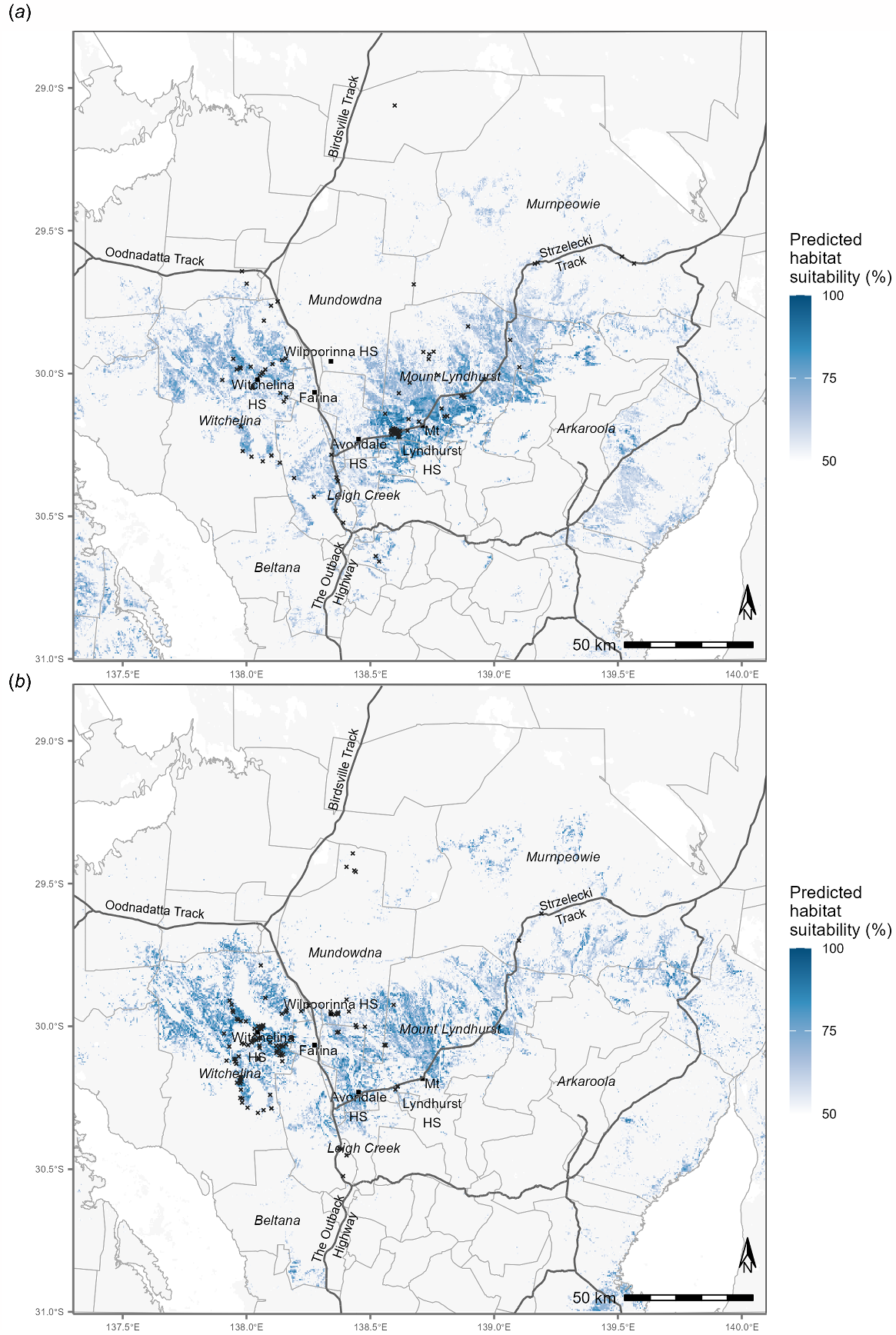
Models were fitted using the predictor data layers at seven levels of aggregation to make predictions of grasswren habitat suitability at grid cell sizes from 80 to 560 m. Assessing these models using OOB errors, a grid cell aggregation to 400 m was chosen for subsequent use. The 1994–2011 fitted model had an OOB error of 15.3% (accuracy 84.7%) and the 2012–2023 model had an OOB error of 11.7% (accuracy 88.3%). Modelled habitat suitability maps (Fig. 2a, b) show the models predictions for the two periods. The 1994–2011 map shows a substantial area of suitable habitat centred on Mount Lyndhurst station and stretching to the northeast on either side of the Strzelecki Track, whereas the 2012–2023 map shows a higher density of suitable grasswren habitat to the west, including on Witchelina.
Grasswren habitat suitability from the random forest models (a) 1994–2011, and (b) 2012–2023. The ‘x’ marks show locations of grasswren observations used for model training.
The spatial distribution and extent of habitat change is highlighted in the prediction differences map (Fig. 3) which suggests both an expansion of suitable habitat in the west and north, and a substantial contraction to the south of the Strzelecki Track.
Map showing the difference in predicted grasswren habitat suitability between the 1994–2011 and 2012–2023 periods. For presentation purposes, areas of the map where predictions are low in both periods have been left unshaded. A, B and C denote selected areas (approx. 25 km2 each) for comparison of the habitat changes between the two modelled periods.
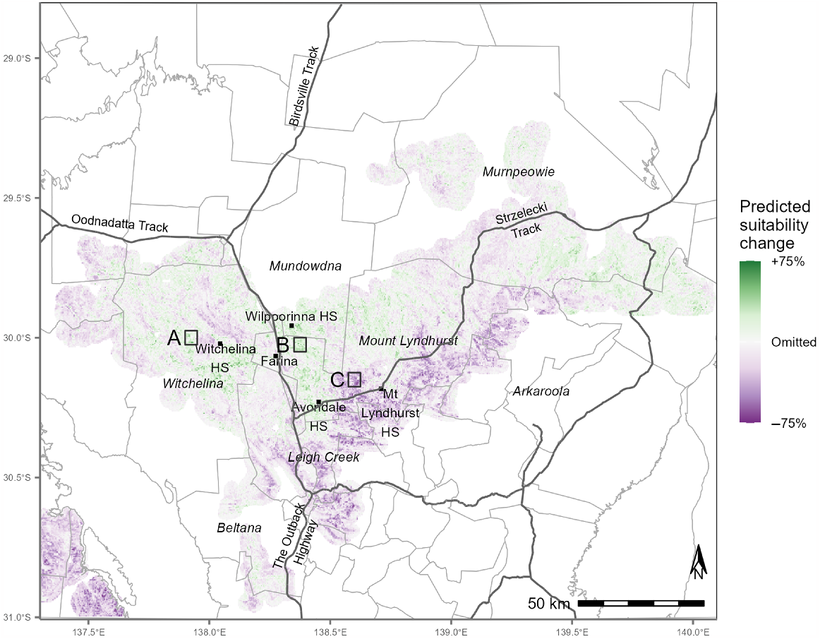
The total areas with grasswren habitat suitability of 50% and 90% decreased in the 2012–2023 period by 25% and 53%, respectively (Table 3). The small area with predicted habitat suitability >90% declined from 15.9 km2 to 7.4 km2. On Witchelina, the absolute area with predicted habitat suitability >50% increased by only 1%, but this represented a proportional increase from 17% to 23% due to greater losses elsewhere. On Witchelina, the area with predicted suitability >90% was 0 in the 1994–2011 period, and 5.6 km2 in the 2012–2023 period (76% of the total 2012–2023 habitat in this suitability class).
| Modelled period | km2 with 50% suitability | km2 with 90% suitability | |
|---|---|---|---|
| Whole study area | |||
| 1994–2011 | 8491 | 15.9 | |
| 2012–2023 | 6352 | 7.4 | |
| Difference (%) | −2139 (−25%) | −8.5 (−53%) | |
| Witchelina reserve | |||
| 1994–2011 | 1433 | 0 | |
| 2012–2023 | 1452 | 5.6 | |
| Difference (%) | 18.3 (1%) | 5.6 (n/a) | |
Important predictor variables
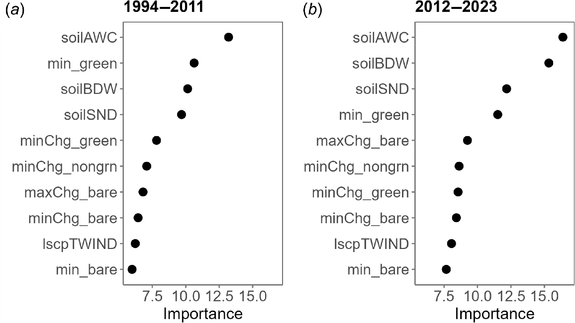
The relative importance of predictor variables was similar between the two modelled periods (Fig. 4). The four most important predictor variables – three soil properties and the FC variable capturing the minimum green vegetation cover – were the same in models for both periods, but with the last being ranked second in the 1994–2011 period and fourth in the 2012–2023 period. The four next most important variables were all of those that captured vegetation change between temporally proximate dry and wet conditions. The two least important variables in both periods were the topographic wetness index and the minimum bare ground cover.
Variable importance plots for Random Forest models for the two periods (a) 1994–2011 and (b) 2012–2023. A higher importance value (‘mean decrease in Gini’) shows that a variable contains more useful information for the model. See Methods and Table 2 for descriptions and abbreviations.
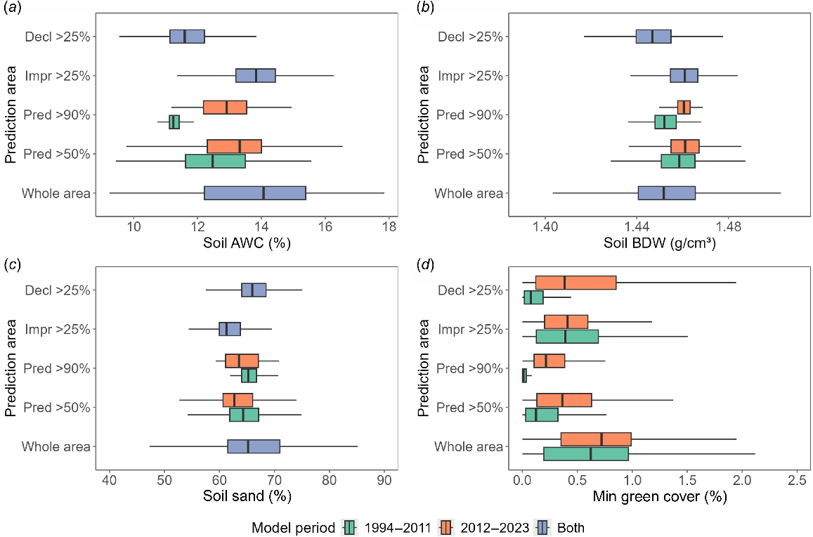
The importance of a variable only indicates the variable contains useful information for a model but does not specify how the values relate to the modelled habitat suitability. Box plots of the four most important variables (Fig. 5) show the relationships between habitat suitability predictions and areas of increase and decline after the early period. The Supplementary material Partial Dependence plots show the response of habitat suitability to each of the predictor variables.
Box and whisker plots of relationships between Random Forest predictions and the four most important predictor variables, showing the range of predictor variable values associated with the whole study area, areas where predicted habitat likelihood was at least 50% and 90% (‘Pred >50%’ and ‘Pred >90%’, respectively) for both modelled periods, and areas where the difference between model predictions showed an improvement or decline of at least 25% (‘Impr >25%’ and ‘Decl >25%’, respectively). (a) Soil available water capacity, (b) soil bulk density, (c) soil sand content and (d) minimum FC green cover (min_green). The boxplot lower and upper hinges correspond to the first and third quartiles, and the whiskers extend from the hinge no further than 1.5 × IQR from the hinge (where IQR is the inter-quartile range, or distance between the first and third quartiles). Outlying data beyond the ends of the whiskers have been omitted.
Relating the most important variables to vegetation cover changes between periods
The three areas A, B, and C selected from the difference map (Fig. 3) show marked change in predicted habitat suitability between the two periods. The mean predicted grasswren habitat suitability in area ‘A’ (on Witchelina) changed from 0.60 to 0.71, in ‘B’ (in northwest Avondale) from a low 0.45 to 0.68, and ‘C’ (Mt Lyndhurst area) from 0.77 to 0.42.
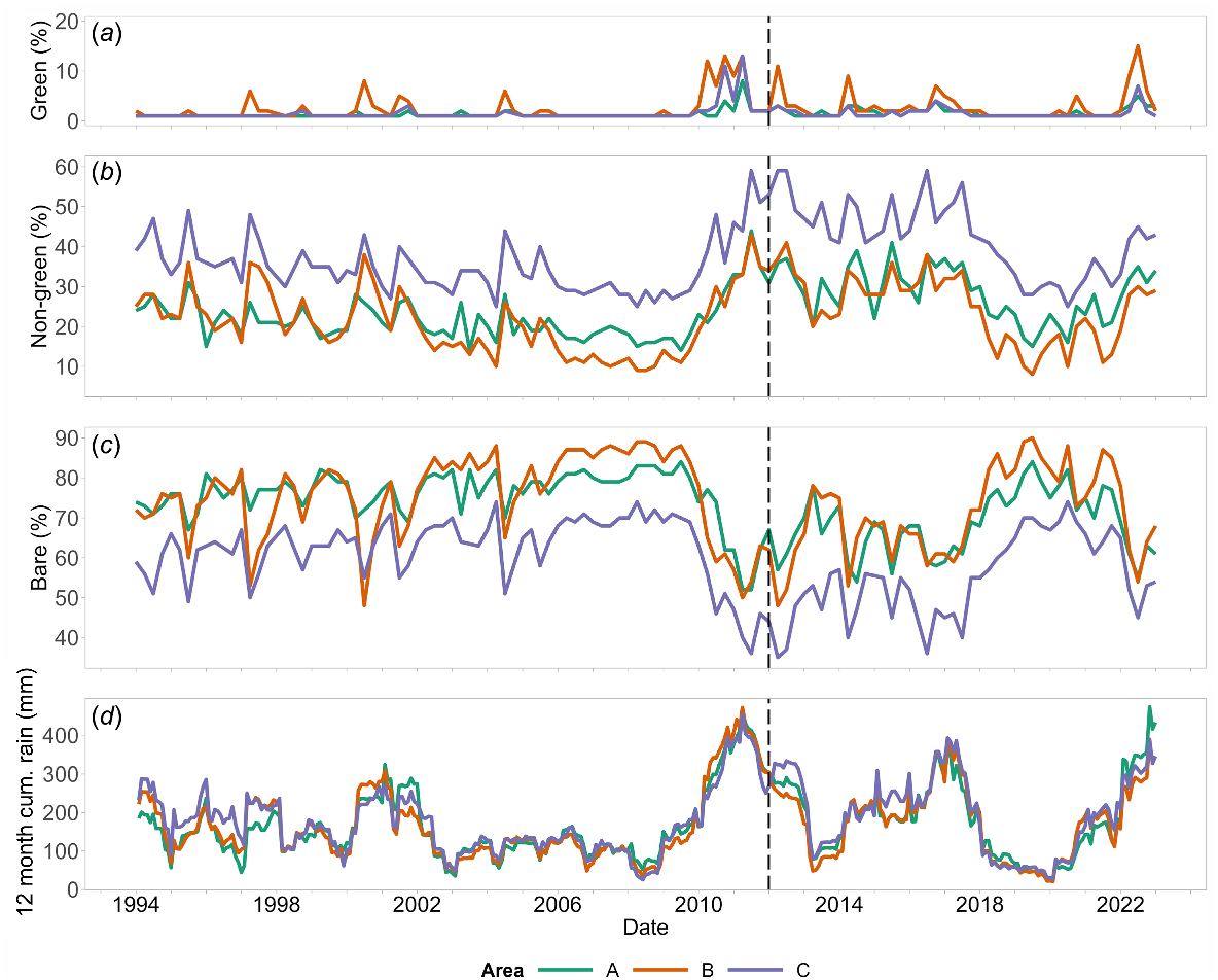
Time-series plots of the three FC classes for areas A, B, and C are shown in Fig. 6 with rainfall (Fig. 6d) for Witchelina (station 17055) 11 km from A; Farina (station 17024) 8 km from B; Mt Lyndhurst (station 17034) 8 km from C. The green cover percentage (Fig. 6a) shows greening-up in response to rain events (Fig. 6d). However, the changes in cover are mostly close to the limit of reliable classification for the Fractional Cover algorithm (mean absolute error = 4.6%) so it is difficult to infer much from this class. The non-green cover and bare ground percentages (Fig. 6b, c) generally vary inversely from one another. From the occurrence of wetter conditions in 2010–2011 and for much of the subsequent 7 years, non-green vegetation cover was higher, and bare ground cover lower than at any other time during the period shown. Between July 2010 and January 2018, area C showed low mean bare ground cover of 47% (σ = 6.6%) compared to both A and B averaging 63% (σ = 5.8% and 7.0%, respectively). Rainfall did not differ substantially between the sites and appeared unrelated to the different changes in grasswren habitat suitability (Fig. 6d).
Time-series plots of percentages of the three fractional cover classes (https://vegmachine.net/; Beutel et al. 2019) from 1994 to 2023 in the three comparison areas A, B, and C (shown in Fig. 3). (a) Green, (b) non-green, (c) bare ground, and (d) 12 month cumulative rainfall calculated for BoM weather stations close to each of the three areas: Witchelina (station 17055) 11 km from A; Farina (station 17024) 8 km from B; Mt Lyndhurst (station 17034) 8 km from C: station 17034 ceased operating from December 2001, so values have been infilled using interpolated rainfall data (Jeffrey et al. 2001).
Model validation survey
Twenty-three field sites were visited during the 2024 survey, 12 of which were within 1 km of the locations of previous grasswren observations and had a mean habitat suitability predicted by the 2012–2023 model of 77% (σ = 17%). Grasswrens were observed during the survey at 8 of those 12 locations. The remaining 11 sites were more than 1 km away from previous grasswren observations, and the 2012–2023 model predicted a mean habitat suitability of 67% (σ = 11%) for these sites. Nine of those 11 sites appeared to be potential grasswren habitat (habitat suitability mean = 72%, σ = 16%), with grasswrens observed at three of these nine sites. The other two sites contained no large chenopods and were not potential grasswren habitat despite the 2012–2023 model predicting a mean habitat suitability of 65% (σ = 12%). The model predictions did not discriminate among the 23 sites as to whether grasswrens were observed or not (, σ = 17% and , σ = 14%, respectively).
Discussion
Principal findings
We used HSM to generate habitat suitability maps for A. m. raglessi for the periods 1994–2011 and 2012–2023. The top four drivers of habitat suitability identified through our modelling were three soil properties and minimum green vegetation cover. Compared with the broader study area, the most suitable grasswren habitat occurs on soils with lower available water capacity, higher bulk density, moderately low sand content, and lower minimum green vegetation cover values. Vegetation cover changes in response to rainfall/drying were also important predictors, but to a lesser degree. This group of important variables suggests that the ability of soils and vegetation to respond to extremes of climatic water stress are key aspects of suitable habitat.
Comparison between maps of the modelled periods showed that suitable habitat declined in previously high-suitability areas whereas expanded in western and northern regions. Notably, Witchelina Station, where post-2010 management aimed to reduce grazing pressure, contained no highest-quality habitat (>90% predicted suitability) in the first period but held 76% of total highest-quality habitat in 2012–2023. While strictly only correlative, this finding implies a positive impact from changed management practices. Conversely, suitable habitat substantially contracted south of the Strzelecki Track, with time-series analysis indicating that vegetation changes, evident as reduced bare ground and increased non-green vegetation, may be linked to grasswren declines there. Higher habitat suitability consistently corresponds with lower minimum green vegetation cover levels across both time periods. Although minimum green cover levels increased slightly overall between the 1994–2011 and 2012–2023 periods, the patterns of change revealed a paradox: areas with the greatest predicted habitat improvements had relatively high green cover initially and showed little change in the 2012–2023 period, while areas with the greatest predicted habitat decline experienced substantial increases in minimum green cover during the second period. It is also counter-intuitive that the most suitable grasswren habitat is predicted on soils with lower-than-average available water capacity, yet areas showing the biggest improvement between periods are those with higher available water capacity. These results reinforce that soil and vegetation responses to extreme climatic water stress may be critical habitat attributes.
Strengths and weaknesses of the study
Our compilation of available observation data revealed notable variation in survey effort of this vulnerable subspecies in time and space. Like all grasswrens, A. m. raglessi is highly cryptic, which creates a challenge for population assessment. Dramatic short-term changes in observed numbers likely reflect changes in detectability in response to climatic extremes rather than actual abundance changes. For example, an increase in frequency of extremely hot days during 2018–2019 was associated with markedly reduced grasswren detection rates on Witchelina reserve (Nankivell and Black 2021) but without a sustained reduction in numbers (G. Carpenter et al. unpubl. data).
Since its acquisition as a nature reserve in 2010, grasswren research has been an intended target in the management of Witchelina. Although higher densities have been observed this likely reflects increased survey efforts, grasswren numbers on Witchelina seemed to decline in 2012 and to fall dramatically in 2019. This suggests that our model results showing a decline in suitable habitat areas are not simply artifacts of survey location bias. Additionally, some areas more frequently accessed by ornithological surveys show clusters of observations within a small area. We have used spatial thinning of the data to reduce bias from repeated closely spaced observations, but the extent to which sampling bias and observability issues influence the model predictions, remains uncertain.
High rainfall years (e.g. 2011–2012, 2016–2017) during the modelled periods could introduce bias in habitat suitability estimates, as grasswrens may temporarily expand into marginal or long-term unsuitable areas during favourable conditions. If grasswren observations are made during those times, this may lead to overestimation of suitable habitat extent and subsequent under- or overestimation of habitat changes when compared with another period.
Despite the limitations in the observation datasets, our approach has yielded several key outcomes. Our field survey in 2024 confirmed the model’s ability to identify new grasswren sites. Most importantly, our modelling has identified key factors driving habitat suitability and changes over time. The areas in which predicted habitat suitability declined are congruent with reports from birdwatchers who have been unable to find grasswrens in those areas on Mount Lyndhurst Station where numbers were high prior to 2012 (P Waanders pers. comm. to AB) and with the sharp decline in grasswren observations made there (Birdlife Australia 2025).
Relationship of findings to other studies
Numerous studies have highlighted the importance of vegetation condition and the impacts of grazing. Habitat degradation from livestock grazing has been shown to impact thick-billed grasswrens (Louter 2016), and the amount of cover and density of chenopod shrubs are important in determining grasswren presence in the field (Black et al. 2011; Slender et al. 2017a). Nankivell and Black (2021) highlighted the potential interaction of climate variables (such as drought and heat stress) and grazing regimes on vegetation condition and composition. Witchelina, which has been managed to reduce grazing intensity since 2010, shows an increase in area of high quality habitat. While data on grazing levels elsewhere in the study area are unavailable, it is highly likely that the impacts of grazing will affect grasswren habitat suitability, and that there will be an interaction between soil attributes, vegetation, and grazing that results in the spatially variable changes in grasswren habitat suitability as modelled in this study.
Previous studies have highlighted that bare ground is an essential attribute of grasswren habitat, approximately 60–80% being found optimal (e.g. see Black et al. 2011; Nankivell and Black 2021). While on-ground methods for assessing bare ground cover in those studies differ from those of the FC datasets (Muir 2011), our time-series analysis shows suitable habitat within a broadly comparable range. In area C, which showed substantial habitat suitability decline, the remotely sensed bare ground cover was well below this range for a prolonged period between 2010 and 2018. The cause of this decrease in bare ground cover in these areas is unknown, but we can speculate that grasses and ephemeral plants that green up readily in wet conditions, and then senesce, leave dry plant material that is detected in the FC data. The observed changes in bare ground and vegetation cover over time demonstrate that understanding vegetation dynamics, and how land management practices influence them, is essential for evaluating and managing grasswren habitat suitability.
Implications
HSM methods such as used in this study are especially suited to the many species for which vegetation dynamics as well as soil and landscape attributes underpin their distribution. Building on this work, it would be of value to better understand grasswren population dynamics and dispersal behaviour, and to more deeply investigate how grasswrens differentially use habitat under different prevailing conditions. Specifically, to determine, if there are key ‘refugia’ habitat types in which grasswrens persist during challenging conditions, and if particular habitat types are used preferentially in better conditions. From a management perspective, it would be good to further ground-truth the application of such model predictions in targeted management options, e.g. rabbit control or focused predator control. Using modelled habitat suitability maps such as these in targeting such management could contribute towards improving biodiversity management for threatened species or other conservation targets.
Conservation organisations and land managers are currently facing the challenges of climate change and changing habitat suitability. It is becoming increasingly important to utilise methods like these to understand how biodiversity adapts and how species distributions shift in the landscape. Such models serve as a foundation for conservation and biodiversity management planning, which can help guide investment in management and programs aimed at creating habitat refuges for biodiversity in a changing landscape.
Conclusions
Our habitat suitability modelling identified key environmental drivers of A. m. raglessi distribution and has demonstrated shifts in suitable habitat area between the 1994–2011 and 2012–2023 periods. Three soil properties and minimum green vegetation cover emerged as the most important predictors of habitat suitability, confirming that habitat response to periods of water stress is key. Field validation demonstrated the models’ predictive capacity and conservation utility.
Comparison between the modelled periods revealed substantial habitat contraction south of the Strzelecki Track and highlights areas requiring conservation attention. Conversely, management-driven habitat improvements are also highlighted, with Witchelina Station transforming from zero highest-quality habitat (1994–2011) to containing 76% of the study area’s most suitable habitat (2012–2023) following reduced grazing pressure.
This research demonstrates HSM’s broader value in understanding threatened species’ responses to landscape-scale changes occurring as a result of interacting climate and management actions. The approach can be applied to other arid zone species facing similar challenges, with increasing importance as climate change intensifies habitat shifts. Despite limitations in the observation data, our integration of long-term datasets with environmental variables provides robust findings for evidence-based management and targeting conservation efforts.
Data availability
Observation data used in this paper are available upon request to the corresponding author.
Conflicts of interest
Alex Nankivell is the current CEO of Nature Foundation, who owns and manages Witchelina Nature Reserve, which forms part of the study area. The other authors declare that they have no conflicts of interest.
Declaration of funding
We received grant funding for surveys from the South Australian Arid Lands Landscape Board and the Wettenhall Environment Trust.
Acknowledgements
Numerous volunteer expert ornithologists contributed to Birds SA, Birdata and ALA observation datasets, without which this analysis would have been greatly limited. Graham Carpenter contributed vital observation datasets, provided comments on early versions of this work, and assisted with planning and carrying out the 2024 field validation survey. Rebecca Trevithick and Terry Beutel helped with Vegmachine access. Jackie Ouzman (CSIRO) provided helpful suggestions on the interpretation of the modelling results. Dr Adrian Fisher and Professor Mike Letnic (UNSW) provided helpful comments on an earlier draft. Valuable support was received from Lyn and Gordon Litchfield of Wilpoorinna Station in allowing access to their family’s properties and providing accommodation during field surveys. D. Hopton, M. Louter, and K. Jones assisted with the 2024 survey. The authors greatly appreciate the input from two anonymous WR reviewers, one of whom put in an exceptional effort and made many informative and constructive suggestions to improve the manuscript.
References
Aiello-Lammens ME, Boria RA, Radosavljevic A, Vilela B, Anderson RP (2015) spThin: an R package for spatial thinning of species occurrence records for use in ecological niche models. Ecography 38, 541-545.
| Crossref | Google Scholar |
Atlas of Living Australia (2023) Occurrence download data. Available at https://doi.org/10.26197/ala.40e4aa76-14e6-4187-ab35-bda419e3af90
Badman FJ (1981) Birds of the Willouran Range and adjacent plains. South Australian Ornithologist 28, 141-153 Available at https://birdssa.asn.au/images/saopdfs/Volume28/1981V28P141.pdf.
| Google Scholar |
Beutel TS, Trevithick R, Scarth P, Tindall D (2019) VegMachine.net. online land cover analysis for the Australian rangelands. The Rangeland Journal 41, 355-362.
| Crossref | Google Scholar |
Birdlife Australia (2025) Birdata. Available at https://birdata.birdlife.org.au/explore [accessed 15 April 2025]
Black A (2011) Subspecies of the Thick-Billed Grasswren Amytornis Modestus (Aves-Maluridae). Transactions of the Royal Society of South Australia 135, 26-38.
| Crossref | Google Scholar |
Black A (2016) Reappraisal of plumage and morphometric diversity in Thick-billed Grasswren Amytornis modestus (North, 1902), with description of a new subspecies. Bulletin of the British Ornithologists’ Club 136, 58-68.
| Google Scholar |
Black A, Carpenter G, Pedler L (2011) Distribution and habitats of the Thick-billed Grasswren Amytornis modestus and comparison with the Western Grasswren Amytornis textilis myall in South Australia. South Australian Ornithologist 37, 60-80.
| Google Scholar |
Black A, Dolman G, Wilson CA, Campbell CD, Pedler L, Joseph L (2020) A taxonomic revision of the Striated Grasswren Amytornis striatus complex (Aves: Maluridae) after analysis of phylogenetic and phenotypic data. Emu - Austral Ornithology 120, 191-200.
| Crossref | Google Scholar |
Black A, Carpenter G, Louter M, Slender A (2025) An appraisal of the hybrid zone between divergent subspecies of Thick-billed Grasswren. South Australian Ornithologist 49, 21-26.
| Google Scholar |
Bradley BA, Olsson AD, Wang O, Dickson BG, Pelech L, Sesnie SE, Zachmann LJ (2012) Species detection vs. habitat suitability: are we biasing habitat suitability models with remotely sensed data? Ecological Modelling 244, 57-64.
| Crossref | Google Scholar |
Breiman L (2001) Random forests. Machine Learning 45, 5-32.
| Crossref | Google Scholar |
Brown CH, Griscom HP (2022) Differentiating between distribution and suitable habitat in ecological niche models: a red spruce (Picea rubens) case study. Ecological Modelling 472, 110102.
| Crossref | Google Scholar |
Chen C, Liaw A, Breiman L (2004) Using random forest to learn imbalanced data. Technical Report. Department of Statistics, University of California, Berkeley, California, USA. Available at https://statistics.berkeley.edu/sites/default/files/tech-reports/666.pdf [accessed 5 December 2023]
Gallant J, Austin J (2012a) Slope derived from 1″ SRTM DEM-S. v4. CSIRO. Data Collection. Available at https://doi.org/10.4225/08/5689DA774564A
Gallant J, Austin J (2012b) Slope relief classification derived from 1″ SRTM DEM-S. v3. CSIRO. Data Collection. Available at https://doi.org/10.4225/08/57512079C1A93
Gallant J, Austin J (2012c) Topographic wetness index derived from 1″ SRTM DEM-H. v2. CSIRO. Data Collection. Available at https://doi.org/10.4225/08/57590B59A4A08
Gill T, Johansen K, Phinn S, Trevithick R, Scarth P, Armston J (2017) A method for mapping Australian woody vegetation cover by linking continental-scale field data and long-term Landsat time series. International Journal of Remote Sensing 38, 679-705.
| Crossref | Google Scholar |
Hijmans RJ, Elith J (2021) Species distribution modeling — R Spatial. Spatial Data Science with R. Available at https://rspatial.org/raster/sdm/index.html [accessed 13 December 2022]
Hirzel AH, Le Lay G (2008) Habitat suitability modelling and niche theory. Journal of Applied Ecology 45, 1372-1381.
| Crossref | Google Scholar |
Jeffrey SJ, Carter JO, Moodie KB, Beswick AR (2001) Using spatial interpolation to construct a comprehensive archive of Australian climate data. Environmental Modelling & Software 16, 309-330.
| Crossref | Google Scholar |
Joint Remote Sensing Research Program (2022) Seasonal fractional cover – Landsat, JRSRP algorithm Version 3.0, Australia coverage. Version 1.0. Available at https://portal.tern.org.au/metadata/23880 [accessed 11 December 2022]
Lawley EF, Lewis MM, Ostendorf B (2011) Environmental zonation across the Australian arid region based on long-term vegetation dynamics. Journal of Arid Environments 75, 576-585.
| Crossref | Google Scholar |
Liaw A, Wiener M (2022) Classification and regression by randomForest; v4.7-1.2. 2, 18–22. Available at https://CRAN.R-project.org/doc/Rnews/
Melville B, Fisher A, Lucieer A (2019) Ultra-high spatial resolution fractional vegetation cover from unmanned aerial multispectral imagery. International Journal of Applied Earth Observation and Geoinformation 78, 14-24.
| Crossref | Google Scholar |
Nankivell A, Black A (2021) Decline of a cryptic desert bird, the Thick-billed Grasswren, in the northern Flinders Ranges, South Australia. South Australian Ornithologist 46, 33-47.
| Google Scholar |
O’Brien L (2021) slga: data access tools for the soil and landscape grid of Australia. v1.2.0. Available at https://github.com/obrl-soil/slga
Pedler L, Watson M, Langdon P, Pedler R (2007) Rare bird surveys, Mt Lyndhurst Station. March 2007. Report prepared for SA Arid Lands Natural Resources Management Board. Available at https://cdn.environment.sa.gov.au/landscape/docs/saal/rare-bird-surveys-mount-lyndhurst-station-2009-rep.pdf
R Core Team (2023) R: a language and environment for statistical computing. version 4.4.1. Available at https://www.R-project.org/
Skroblin A, Murphy SA (2013) The conservation status of Australian malurids and their value as models in understanding land-management issues. Emu - Austral Ornithology 113, 309-318.
| Crossref | Google Scholar |
Slender AL, Louter M, Gardner MG, Kleindorfer S (2017a) Patterns of morphological and mitochondrial diversity in parapatric subspecies of the Thick-billed Grasswren (Amytornis modestus). Emu - Austral Ornithology 117, 264-275.
| Crossref | Google Scholar |
Slender AL, Louter M, Gardner MG, Kleindorfer S (2017b) Plant community predicts the distribution and occurrence of thick-billed grasswren subspecies (Amytornis modestus) in a region of parapatry. Australian Journal of Zoology 65, 273 282.
| Crossref | Google Scholar |
Sohoulande Djebou DC, Singh VP, Frauenfeld OW (2015) Vegetation response to precipitation across the aridity gradient of the southwestern United states. Journal of Arid Environments 115, 35-43.
| Crossref | Google Scholar |
Valavi R, Elith J, Lahoz-Monfort JJ, Guillera-Arroita G (2021) Modelling species presence-only data with random forests. Ecography 44, 1731-1742.
| Crossref | Google Scholar |
Valavi R, Guillera-Arroita G, Lahoz-Monfort JJ, Elith J (2022) Predictive performance of presence-only species distribution models: a benchmark study with reproducible code. Ecological Monographs 92, e01486.
| Crossref | Google Scholar |
Viscarra Rossel R, Chen C, Grundy M, Searle R, Clifford D, Odgers N, Holmes K, Griffin T, Liddicoat C, Kidd D (2014a) Soil and landscape grid national soil attribute maps – available water capacity (3″ resolution) – Release 1. v6. CSIRO. Data Collection. Available at https://doi.org/10.4225/08/546ED604ADD8A
Viscarra Rossel R, Chen C, Grundy M, Searle R, Clifford D, Odgers N, Holmes K, Griffin T, Liddicoat C, Kidd D (2014b) Soil and landscape grid national soil attribute maps – bulk density – whole earth (3″ resolution) – Release 1. v5. CSIRO. Data Collection. Available at https://doi.org/10.4225/08/546EE212B0048
Viscarra Rossel R, Chen C, Grundy M, Searle R, Odgers N, Holmes K, Griffin T, Liddicoat C, Kidd D, Clifford D (2014c) Soil and landscape grid national soil attribute maps – clay (3″ resolution) – Release 1. v6. CSIRO. Data Collection. Available at https://doi.org/10.4225/08/546EEE35164BF
Viscarra Rossel R, Chen C, Grundy M, Searle R, Odgers N, Holmes K, Griffin T, Liddicoat C, Kidd D, Clifford D (2014d) Soil and landscape grid national soil attribute maps – sand (3″ resolution) – Release 1. v6. CSIRO. Data Collection. Available at https://doi.org/10.4225/08/546F29646877E