
Testing the efficiency of thermal imagers for detecting arboreal marsupials in temperate forests
Nicholas Tan A , José J. Lahoz-Monfort B C and Brendan A. Wintle B *
A
B
C
Abstract
Wildlife monitoring must be cost-efficient due to constrained conservation budgets. Part of efficient monitoring is the selection of appropriate and effective methods for monitoring species.
In this paper, we evaluated the effectiveness of two methods (spotlighting and thermal imaging) for detecting four species of arboreal marsupial in the Strathbogie region of north-eastern Victoria, Australia.
We conducted 108 visits to 15 survey locations across the study area over the period of November 2017–June 2018. Each survey was conducted as a 250 m transect over 20–30 min. Occupancy modelling was used to evaluate the influence of observation method choice on detectability while accounting for other covariates. We calculated the expected minimum number of visits required to achieve a low (0.1) probability of failing to detect each of the four target species when present.
We found that spotlighting was best used for detecting greater gliders and ringtail possums, whereas thermal imagers were best for detecting mountain brushtail possums and koalas. Detectability estimates indicated that a minimum of three spotlighting or four thermal surveys should be planned.
The choice of method for detecting arboreal marsupials is dependent on several factors, including the body mass and eye shine of the target species. Covariates may play a part in detectability of some species, although the greater glider remains highly detectable regardless of the method.
Behavioural and physiological differences between arboreal species can influence the effectiveness of the survey method. Foraging activity and response to stimuli such as spotlights affect detectability and should be considered when planning survey methodology.
Keywords: arboreal marsupials, comparative study, detectability, greater gliders, occupancy, spotlight, thermal imagers, wildlife monitoring.
Introduction
Wildlife monitoring is essential for understanding and managing species and their threats (Yoccoz et al. 2001). With limited resources allocated to monitoring, high efficiency is paramount, including the choice of method. (Devictor et al. 2010; Dickinson et al. 2010). Detectability of species and the efficiency of a given method in each context relies on a number of factors that can influence not only results, but also implementation of the method (Lancia et al. 2005).
When choosing a monitoring method, detectability is one of the most important considerations and has two main components, namely, availability and conditional capture probability (Pollock et al. 2004; Kéry and Schmidt 2008). Availability refers to the chance that a species is in the area (or occupancy), whereas conditional capture probability is the probability of detecting a target species, given its presence. Several factors, including density, physiology or behaviour of animals, site-level variables, or survey-level variables, could affect an observer’s ability to detect animals. Each of these factors can alter one or both components of detectability (Engeman and Witmer 2000; Witmer 2005; Wintle et al. 2005; O’Donnell et al. 2015; Helle et al. 2016).
Because of this, methods that detect animals by using different measurements (light, heat, audio) can have different detectability rates. For example, frogs can be detected visually by using camera, audibly by listening or using recording devices, or by using eDNA, and detectability can differ depending on the method (Vences et al. 2008; Bálint et al. 2018). Understanding the influence of a detection method on detectability, and therefore survey efficiency, is critical to designing efficient monitoring programs that maximise value (Block et al. 2001; Swann et al. 2004; Burton 2012). This necessitates quantitative evaluation of monitoring.
Wildlife monitoring has undergone many advances over the years, with a significant increase in the number of monitoring methods (Legg and Nagy 2006; Liu et al. 2008; O’Connell et al. 2010; Adams et al. 2012; Burton et al. 2015; Linchant et al. 2015). Many of these tools improve the power of monitoring by providing more reliable observation data and higher detectability. Thermal imaging is one such technological advance. It creates a visible image of the thermal infra-red band on a display, called a thermogram, on the basis of the amount of radiation an object emits. Animals tend to emit more radiant heat in relation to their surroundings at night, and can therefore be readily distinguished on thermal imagery.
The ability of thermal sensors to be used in conditions with limited or no light makes them well suited for surveys occurring at night or in other dark areas such as caves. Thermal sensors can reduce the chance of adversely affecting animal behaviour compared with traditional white-light spotlighting (Blom et al. 2004; Martin and Réale 2008). However, thermal imagers area more expensive than are spotlights (Cilulko et al. 2013). If they are to be used in preference to cheaper spotlights, it will be important that they are substantially more effective in detecting target animals.
Size and surroundings play a part in thermal detectability (Cilulko et al. 2013). Small animals or animals that radiate less heat owing to thicker fur (which reduces the amount of heat radiated), may show up less prominently on the image. The amount of detail on the image depends on the imager. In lower-quality imagers, object definition can be poor, making it difficult to identify some species without clear, identifiable features such as distinct body shapes, or in combination with other cues such as auditory cries. Similar looking species can result in false identification unless one gets closer to accurately tell them apart.
Comparative studies have examined the effectiveness of thermal imagers. Boonstra et al. (1994) looked at a variety of small mammals, including hares and squirrels, with thermal imagers and compared effectiveness among seasons. Collier et al. (2007) found that thermal imagers were almost twice as effective when detecting white-tailed deer. A significant increase in detection rate and distance for red deer, brown hare, European rabbit and wild boar was found by Focardi et al. (2001), but they concluded that the cost of using thermal imagers needed to be justified by a notable increase in detections and offsetting of labour costs.
Arboreal animals provide an additional challenge to monitoring efforts because they can exist high up in dense canopies, making them difficult to see. Surveyors must look up as well as around them, which can slow survey work. Tree foliage also provides a physical barrier to detectability. With an increasing number of studies showing sensitivity to changes in landscape and a push to preserve native forests because of their impact on arboreal marsupial populations, there is a need for robustness in arboreal mammal monitoring to accurately monitor changes in sensitive populations (Lindenmayer et al. 2003, 2024).
Standard monitoring methods for arboreal species usually utilise spotlight and/or camera trapping (Harley et al. 2014), although sometimes thermal monitoring is used. Over the past several years, there has been an increase in the literature on the comparative effectiveness of thermal imagers, especially for detecting arboreal marsupials in the Phalangeriformes suborder, which includes possums and gliders (Drury 2016; Witt et al. 2020; Underwood et al. 2022; Dawlings et al. 2024). Other marsupials in these studies include greater gliders (Vinson et al. 2020). Other Australian animals have also been used as a basis for comparing the two methods, such as the greater bilby (Augusteyn et al. 2020; McGregor et al. 2021; Dawlings et al. 2024).
Thermal imagers offer potential as an alternative monitoring method for arboreal species, because they are comparatively less invasive than spotlighting, and allow better coverage than does camera trapping (which may have problems with height restrictions). More studies on such comparative methods can still be useful, especially as variables affecting effectiveness of either method can differ depending on the site or time of survey.
This research aimed to compare the efficiency of spotlighting and hand-held thermal imaging for detecting a set of arboreal marsupials, in temperate forests in north-eastern Victoria. We considered how the choice of method affects efficiency and detectability of monitoring of arboreal marsupial species in the area by using occupancy-detection modelling.
Materials and methods
Target species
We estimated detection rates for the following four forest-dependent arboreal marsupials: the mountain brushtail possum (Trichosurus cunninghami), common ringtail possum (Pseudocheirus peregrinus), greater glider (Petauroides volans), and the koala (Phascolarctos cinereus). The greater glider is listed as Endangered since 2022, having previously been Vulnerable under Australia’s List of Threatened Fauna (Environment Protection and Biodiversity Conservation Act 1999), owing to reduction in population sizes over the past few decades (Wagner et al. 2020). As such, it has been the focus of several studies over the past few years (Ashman et al. 2021; Vinson et al. 2021; Norman and Mackey 2023).
Differences in biology, morphology and behaviour among species may influence their detectability (Garrard et al. 2013; Sólymos et al. 2018). Examples include koalas’ large body (the size being typically between 60 and 85 cm and body mass over 6 kg), but tendency to look away from incoming light sources. This may increase their detectability with thermal imaging but decrease their detectability with spotlighting, which relies on seeing the animals eyeshine.
Surveys were conducted in the Strathbogie State Forest in north-eastern Victoria, Australia (Supplementary material, Fig. S1), an area of about 326 km2, approximately 28 km east of Euroa. It is a wet eucalypt forest, chosen because it was an ideal location for surveying greater gliders, which were prominent in the area.
We surveyed from November 2017 to June 2018, across 15 different sites, which were chosen for variability in habitat type and ease of accessibility (Table S1). Maximum temperature during this period ranged from to 16.2°C (June 2018) to 38.9°C (January 2018). Each site was visited at least three times and up to five times, for a total of 108 surveys. Three or four sites were visited on any given night. Surveys were conducted using a LED LENSER H7R spotlight with a wattage of up to 1000 lm, and a PULSAR Helion XQ19F hand-held thermal scope. This brand of thermal scope did not have a zoom function, but did have variable magnification. It has a resolution of 640 × 480, and a working temperature range of −25–50°C.
Wind speed, cloud cover, temperature, and moon phase were all recorded at the start of each survey (Table 1), by using data loggers and weather logs as necessary. Because of seasonality, surveys were started approximately 2 h after sunset each day. Although time of survey was recorded, it was not considered as a covariate. We randomised the order in which the sites were visited to account for changes in species behaviour that may affect detectability over the course of the night. We collected site-level covariate data, including distance of the site from the main road as a proxy for human disturbance.
| Variable | Nature and levels | Reasoning/past papers | Acquisition method | |
|---|---|---|---|---|
| Method | Discrete, spotlight and thermal | Basis of study | Randomly assigned during surveys | |
| Moon phase | Discrete, new moon, half moon, full moon | Affects visibility (amount of light), animal behaviour (Zimmermann 2010) | Observed during surveys | |
| Cloud cover | Continuous. Ranged from 0 (clear skies) to 100 (overcast) | Affects visibility (Wayne et al. 2006) | Estimated during surveys | |
| Temperature | Continuous. Ranged from 2°C to 11°C over the study | Affects effectiveness of thermal imagers and animal behaviour (Wayne et al. 2006) | Data loggers and weather records | |
| Wind speed | Continuous. Ranged from 0 to 20 mph over the study | Possibly affects temperature and spotlighting (Sokos et al. 2015) | Data loggers and weather records | |
| Observer | Discrete, experienced (author) and others | Different experience level can affect spotlighting (Sunde and Jessen 2013) | Assigned during surveys | |
| Distance of site from main road | Continuous | Used as a proxy to estimate level of human disturbance | GPS and Google Earth measurements |
| Species | Spotlight detectability | Thermal detectability | |
|---|---|---|---|
| Greater glider | 0.99 | 0.94 | |
| Ringtail | 0.6 | 0.45 | |
| Brushtail | 0.31 | 0.41 | |
| Koala | 0.2 | 0.41 |
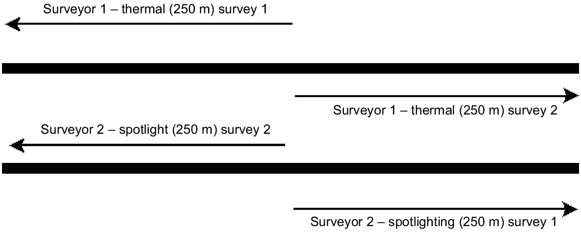
During each visit, surveys commenced at approximately the middle of the 500 m transect at each site (Fig. 1). Each of two observers proceeded in opposite directions by using either spotlight or the thermal imager. Allocation of the method to observer was determined randomly at each survey occasion, to reduce the potential for influence of one observer’s observations on the other observer’s search pattern (although an observer effect was still included in the modelling to account for the possibility). On reaching 250 m, both observers returned to the starting point, then walked the other 250 m that was just walked by the other observer. This minimised interference between observers. Observer experience with either method was not noted as a covariate, although most observers had some experience with spotlighting and found the thermal imager operation and use intuitive.
Surveyors start at the middle of the transect and perform individual surveys in opposite directions, one using a thermal imager and the other a spotlight as the primary detecting method, before returning to the centre. Each of these represents a repeat survey. The surveyor performs a repeat survey in the opposite direction, to cover the other half of the site. Each visit to a site by two observers yielded four surveys.
When an individual of any species was observed, it was identified and the perpendicular distance of the first detection noted. Two distance measurements were taken using a laser rangefinder; the direct distance from the observer to the individual, and the distance from the observer to the base of the tree where the animal was located. Individuals detected on return trips were not counted. Each visit of a site provided four observations (two observers × two 250 m transects); for this study, collections of individual detections were summarised as ‘species detected’ (1) or ‘species not detected’ (0), for each of the four observations.
Modelling detectability
The influence of observation method and weather, environment, and observer covariates was modelled using occupancy (MacKenzie et al. 2002; MacKenzie and Royle 2005).
Modelling was conducted for each of the four target species independently. Analyses were performed using the ‘unmarked’ (ver. 1.5.0, see https://cran.r-project.org/web/packages/unmarked/index.html; Fiske and Chandler 2011) package in R (ver. 0.12–0) with the function occu.
The occupancy model can be seen as two linked logistic regressions within a hierarchical framework (Guillera-Arroita 2017). At the site level, the (true, often latent) occupancy status of a site i, zi, can be described by the probability of occupancy , which may be linked to site-level covariates in Eqn 1, as follows:
At the observation level, the data (detection/non-detection ) can be described with the probability of species detection at that site i and survey occasion j (, conditional on presence of the species), which itself may be linked to covariates (site- or occasion-level), where in Eqn 2
where logit represents logit link function.
Because the focus on this study was on detectability, all occupancy models estimated a single, mean occupancy rate for each species and only covariates on detectability were estimated.
Effect plots were created for each of the four target species, to look at the contribution of each covariate in the full model on detectability (i.e. the model with all covariates included in detectability).
Whereas the generated effects plots give an idea of the general effect each covariate has on detectability, the full model may not necessarily be a good fit owing to the large number of parameters involved, potentially leading to overfitting. To examine models that may more accurately fit the effect of the relevant covariates, a model selection process was performed on the basis of Akaike information criterion (AIC) rank (Akaike 1987). Because the sample size for this survey was not particularly large for some species (particularly T. cunninghami and P. cinereus), the AIC corrected (AICc), which corrects for small sample size, was used instead (Finley et al. 2005; Yates and Muzika 2006; Boulanger et al. 2008).
We considered linear, quadratic and cubic relationships for detectability covariates (on the logit scale). We assumed that detection covariates had a negligible effect on occupancy. Model selection was conducted by fitting all possible combinations of covariates (using the dredge function in the R package ‘MuMIn’ (ver. 1.48.11, https://cran.r-project.org/web/packages/MuMIn/index.html; Barton and Barton 2015)), and then ranking them according to AICc. To select the best-fitting models, only models with ΔAICc < 4 were considered (where ΔAICc is the difference in AIC units relative to the top-ranking (lowest AIC) model). Akaike weights were then calculated for each model by using the following Eqn 3, as follows:
where wi represents the weight of each model relative to all the models kept in that set.
To interpret estimated detection probabilities into the mimimum survey effort that should be committed in the design of a monitoring program, a plot of cumulative detection probability (the probability M that a species would remain undetected after n visits, given a single-visit with detection probability p) was created for each of the four target species under both of the candidate detection methods in Eqn 4, as follows:
The single-visit detection probability (p) used to construct detection curves was estimated assuming typical conditions encountered during surveys. Temperature was set to 11°C, and method was fixed to either spotlighting or thermal image.
We also considered the deviance reduction % of the best model from the null model (when no covariates are fitted). This determines how much of the variation in results can be explained by the best-fit model’s addition of covariates. This is determined by the following Eqn 5:
where a represents a model and null is the null model with no added covariates. Deviance for each model is calculated with 2*-logLik, a representation of the log likelihood, and is given in the R output. The result is then multipled by 100 to give the deviance reduction % for a given model from the null model.
Results
Survey results
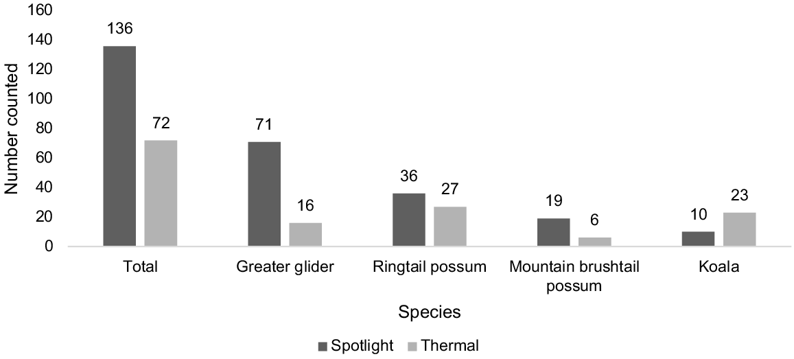
In total, 208 individual animals were detected across 108 surveys of 15 survey locations. Twelve detections of animals, nine from spotlighting and three from thermal, which could not be clearly identified, were not included in the dataset. Greater gliders and common ringtails were detected at all sites. Mountain brushtails and koalas were detected at 11 and 12 of the 15 sites respectively. Fig. 2 shows the total counts of individual animals throughout the surveying period, split by species and method.
Modelling results
A significant relationship between ‘observation method’ and detectability was observed for each species. An estimation of the regression coefficient of each covariate for each species can be seen in Fig. 3.
Estimated regression coefficients of each of the variables that influence detectability in the full model for each species. Dots provide the point estimates and lines represent the 95% confidence interval. When lines do not cross 0, the variable is considered statistically significant and P < 0.05.
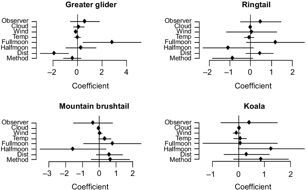
Table 3 shows the best fit models for all species, as well as the best fit models where method is a covariate. Method was the strongest effect for brushtails and the only effect included in the model for koalas, whereas fullmoon and halfmoon were the strongest effects for the AIC-best models for greater gliders and ringtails respectively.
| Species | Best-fit model | Best-fit model (must include Method) | Delta AIC of Method model from AIC-best model | % Deviance reduction of AIC-best model | |
|---|---|---|---|---|---|
| Greater Glider | logit (pij) = 1.58–1.54 × Method ij+ 2.77 × Fullmoon ij – 0.15 × Wind ij | logit (pij) = 1.58–1.54 × Method ij + 2.77 × Fullmoon ij – 0.15 × Wind ij | 0 | 19.8 | |
| Ringtail | logit (pij) = −0.13 + 1.23 × Fullmoon ij – 0.97 × Halfmoon ij | logit (pij) = 0.39–0.61 × Methodij – 1.26 × Halfmoon ij | 2.03 | 7.7 | |
| Brushtail | logit (pij) = −2.86 + 0.21 × Temp ij | logit (pij) = −3.07 + 0.41 × Method ij + 0.21 × Temp ij | 3.09 | 3.8 | |
| Koala | logit (pij) = −1.38 + 1.02 × Method ij | logit (pij) = −1.38 + 1.02 × Method ij | 0 | 4.1 |
Also includes the % deviance reduction of the best-fit model, from the model where no covariates are included.
AIC-best models were small relative to the number of variables considered to be likely to influence detectability for each species (Table 3). The AIC-best model for each species explained between 3.8% and 19.8% of the variation in detectability (Table 3). The low variation explained can be attributed to a large amount of noise or other factors during the study, some of which is unexplained or were not measured at the time.
The models within four AICc units (ΔAICc < 4) of the top-ranking ones after model selection were considered further; AIC weights were calculated for that set of models, and the full results (ΔAICc < 4) can be found in Table 4.
| Species | Model | DeltaAIC | Weight | Cloud | Dist | Fullmoon | Halfmoon | Method | Observer | Temp | Wind | |
|---|---|---|---|---|---|---|---|---|---|---|---|---|
| Glider | 1 | 0.00 | 0.62 | ✓ | ✓ | ✓ | ||||||
| 2 | 1.48 | 0.30 | ✓ | ✓ | ||||||||
| 3 | 4.00 | 0.08 | ✓ | ✓ | ✓ | |||||||
| Inclusion rate (%) | 0 | 33 | 100 | 0 | 100 | 0 | 0 | 33 | ||||
| Ringtail | 1 | 0.00 | 0.19 | ✓ | ✓ | |||||||
| 2 | 0.42 | 0.15 | ✓ | |||||||||
| 3 | 0.44 | 0.15 | ✓ | |||||||||
| 4 | 2.03 | 0.07 | ✓ | ✓ | ||||||||
| 5 | 2.48 | 0.05 | ✓ | ✓ | ||||||||
| 6 | 2.49 | 0.05 | ✓ | ✓ | ✓ | |||||||
| 7 | 2.54 | 0.05 | ✓ | ✓ | ||||||||
| 8 | 2.88 | 0.05 | ✓ | |||||||||
| 9 | 3.27 | 0.04 | ✓ | ✓ | ✓ | |||||||
| 10 | 3.33 | 0.04 | ✓ | ✓ | ||||||||
| 11 | 3.51 | 0.03 | ✓ | ✓ | ||||||||
| 12 | 3.54 | 0.03 | ✓ | ✓ | ||||||||
| 13 | 3.65 | 0.03 | ✓ | ✓ | ||||||||
| 14 | 3.75 | 0.03 | ✓ | ✓ | ||||||||
| 15 | 3.83 | 0.03 | ✓ | ✓ | ||||||||
| Inclusion rate (%) | 13.30 | 20.00 | 53.20 | 60.00 | 20.00 | 0.00 | 20.00 | 13.30 | ||||
| Brushtail | 1 | 0.00 | 0.14 | ✓ | ||||||||
| 2 | 0.46 | 0.11 | ✓ | |||||||||
| 3 | 0.56 | 0.11 | ✓ | |||||||||
| 4 | 1.02 | 0.08 | ||||||||||
| 5 | 1.09 | 0.08 | ✓ | ✓ | ||||||||
| 6 | 1.41 | 0.07 | ✓ | ✓ | ||||||||
| 7 | 2.29 | 0.04 | ✓ | |||||||||
| 8 | 2.46 | 0.04 | ✓ | ✓ | ||||||||
| 9 | 2.64 | 0.04 | ✓ | ✓ | ||||||||
| 10 | 2.68 | 0.04 | ✓ | ✓ | ||||||||
| 11 | 2.83 | 0.03 | ✓ | ✓ | ||||||||
| 12 | 3.09 | 0.03 | ✓ | ✓ | ||||||||
| 13 | 3.31 | 0.03 | ✓ | ✓ | ||||||||
| 14 | 3.36 | 0.03 | ✓ | ✓ | ||||||||
| 15 | 3.49 | 0.02 | ✓ | ✓ | ||||||||
| 16 | 3.57 | 0.02 | ✓ | |||||||||
| 17 | 3.62 | 0.02 | ✓ | ✓ | ||||||||
| 18 | 3.63 | 0.02 | ✓ | ✓ | ||||||||
| 19 | 3.98 | 0.02 | ✓ | |||||||||
| 20 | 3.99 | 0.02 | ✓ | |||||||||
| Inclusion rate (%) | 25.00 | 25.00 | 5.00 | 10.00 | 20.00 | 10.00 | 40.00 | 20.00 | ||||
| Koala | 1 | 0.00 | 0.19 | ✓ | ||||||||
| 2 | 0.39 | 0.15 | ✓ | |||||||||
| 3 | 1.11 | 0.11 | ✓ | ✓ | ||||||||
| 4 | 1.96 | 0.07 | ||||||||||
| 5 | 2.11 | 0.06 | ✓ | ✓ | ||||||||
| 6 | 2.21 | 0.06 | ✓ | ✓ | ||||||||
| 7 | 2.93 | 0.04 | ✓ | |||||||||
| 8 | 3.07 | 0.04 | ✓ | ✓ | ||||||||
| 9 | 3.20 | 0.04 | ✓ | ✓ | ✓ | |||||||
| 10 | 3.44 | 0.03 | ✓ | ✓ | ||||||||
| 11 | 3.48 | 0.03 | ✓ | ✓ | ||||||||
| 12 | 3.68 | 0.03 | ✓ | ✓ | ||||||||
| 13 | 3.70 | 0.03 | ✓ | ✓ | ||||||||
| 14 | 3.77 | 0.03 | ✓ | ✓ | ||||||||
| 15 | 3.81 | 0.03 | ✓ | ✓ | ||||||||
| 16 | 3.89 | 0.03 | ✓ | ✓ | ||||||||
| 17 | 3.98 | 0.03 | ✓ | ✓ | ||||||||
| Inclusion rate (%) | 23.60 | 11.80 | 5.40 | 27.00 | 48.60 | 32.40 | 11.80 | 5.40 |
The top-ranked models by ΔAICc for each target species, and the covariates included in each model, along with their relative weight for that each species. Only models within four ΔAICc units of the top one are presented. Ticks represent covariate included in each particular model for the species. As an exploration of relative covariate importance, the last row for each species shows the sum of weights for each covariate and an indicator of that covariate’s occurrence rate on the bottom.
For greater gliders, method and fullmoon were included in all models, whereas distance from main road and wind were included only once; the rest of the covariates did not appear in any of the models (Table 4).
For mountain brushtail possums, temperature was the most common covariate, appearing in 40% of the models; the rest of the covariates appeared anywhere from 5% to 25% of the time, with method appearing 20% of the time.
Halfmoon and fullmoon had the highest occurrence rate in ringtail possum models, with a 53.2% and 60% occurrence rates respectively; method was in 20% of the models.
Method was the most common covariate in the top-ranked models for koalas, appearing in 48.6% of the models within the cut-off.
Cumulative detection plots showed that greater gliders had a low probability (<0.1) of being missed after the first visit (Fig. 4). To ensure that the probability of missing the species if present at the site was less than 0.1, ringtail possums required three visits with a spotlight and four visits with a thermal imager, mountain brushtail possums required six visits for spotlight and four visits with the thermal, and koalas required ten visits for spotlight and four visits with the thermal.
Estimated graph showing the probability of failing to detect a target species (y-axis) that is present at a site after a certain number of visits to a site (x-axis), using either spotlighting or thermal imaging as a method, on the basis of the best-fit model (based on ΔAICc) for each species by using method as a variable. A line is drawn at probability = 0.1 as a cut-off point for a low probability of missing the species.
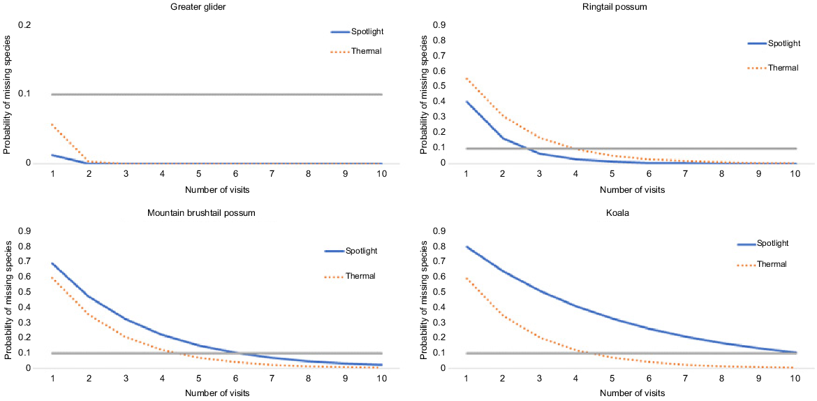
Spotlighting was more efficient for detecting greater gliders and ringtails, and thermal for detecting brushtails and koalas (Table 2, Fig. 4). These are based on the best-ranked model (using ΔAICc) that included method as a factor, for each species (Table 3).
Discussion
Differences in the results can be inferred for each species by using knowledge of both physiology and behaviour and the factors that influence the effectiveness of each method. Koalas and brushtails were best detected using the thermal imager, most likely because of their larger body size and mass (60–85 cm and 40–55 cm respectively), than those of greater gliders (30–43 cm) and ringtails (30–35 cm) (Gynther and Baker 2013). Objects of larger mass produce more thermal energy that creates a more striking image on the thermogram. This causes higher per-individual detectability for larger species by using the thermal imager, particularly for koalas, who weigh, on average, about 6.16 kg for females and 7.08 kg for males, compared with 1.36 kg for greater gliders (Ellis and Bercovitch 2011; McGregor et al. 2020).
Thermal imagers may have reduced effect when looking at objects further up in the canopy from the ground, as greater gliders forage high in the canopy and this, coupled with their smaller body size, means they are more likely to be obscured by vegetation which therefore reduces their relative detectability by using thermal imagers.
The main factor in spotlighting detectability is eyeshine. Greater gliders have very notable eyeshine, and so are easily detected with spotlighting. Furthermore, they do not shy away when exposed to spotlighting, thus leading to a long period in which they are visible under spotlight, allowing for both higher detectability and easier identification. Ringtail possums and mountain brushtail possums have noticeable eyeshine (although not to the degree of greater gliders). They also tend to forage closer to the ground, making them easily detected with spotlights and thermal imaging. Koalas do not usually give off as much eyeshine as do the other target species and tend to look away from direct spotlighting. This can result in missed detections of individuals when spotlighting and thus imperfect detection of the species. This might explain why koalas were most likely to be detected using thermal imaging in this study.
Greater gliders still maintained a very high detectability regardless of the method (see Table 2), with detectabilities of 0.99 (spotlighting) and 0.94 (thermal) under optimal conditions. This might indicate that despite possible physiological and behavioural factors, greater gliders remain highly detectable regardless of the method.
For mountain brushtail possums, detectability was low across both methods (Table 2), with average detectability of 0.27 with spotlighting and 0.36 with thermal imaging (average estimated values at a temperature of 11°C). Although they do not tend to look away from the spotlight, they are larger than ringtail possums and greater gliders, which could explain why thermal detectability was slightly higher for mountain brushtail possums than was detectability by spotlighting.
Survey method was a common and strong factor in detectability among the top models for greater gliders and koalas, appearing in 100% of the top models for greater gliders, and 48.6% top models for koalas (Table 2 in Appendix). In contrast, method appears only in 20% of the top models for ringtail possums and mountain brushtail possums.
Moon phase and temperature were influential factors in models for greater gliders, ringtails, and brushtails (Table 3). The amount of light and ambient heat during the time of survey influence detectability by modifying animal activity. Warmer temperatures may encourage animals to forage more actively, and a bright moon may supress activity becaue of predator avoidance. Although not recorded for this survey, the range and rate of change of temperature over the day may also affect activity. Future studies along this vein may include this as a covariate to examine whether this may have a significant impact, especially in light of climate change trends (Śmielak et al. 2023). Some other variables that may influence detectability of our target species, such as tree density and average height (Wintle et al. 2005), were not collected during this study.
Detectability-only logistic regression models explained a relatively small portion of the overall variation in detection data (Table 3, right-hand column). This is unsurprising given that many factors influence detectability, some of which were not recorded in this study, including high inherent randomness of species movement and their exact location during a given survey, the presence of other animals in the study site at or before the time of survey, and the readiness and alertness of observers on the night of survey. These factors could be investigated in other future studies.
Beyond detectability considerations, logistic factors may influence study design to favour a particular method, particularly if studies occur over large areas. The learning burden is relatively low for both methods tested here. However, other factors such as the burden of carrying extra equipment (e.g. a thermal imager) and equipment costs may affect method choice. Thermal imagers have been made more accessible in recent times but remain more expensive than spotlights. The thermal imager used in this study (PULSAR Helion XQ19F) cost just above AUD4,000 during the period of survey, compared with about AUD140 for the spotlight used (LED LENSER H7R). The difference in cost, especially if outfitting multiple surveyors, would be a consideration for many organisations. For most species studied here, the cost of thermal imaging may not be justified, given the relatively small gain in detection probability for just one or two species.
Another species observed during these surveys (but not analysed owing to lack of detection data) was the feathertailed glider (Acrobates pygmaeus). They have small bodies (weighing about 13 g), but very little eyeshine, making them poor targets for spotlighting (Ward 2000). However, they show up very well on the thermogram, which is likely owing to their high surface area and thinner fur, allowing more heat radiation (Gynther and Baker 2013). They also tend to be quite active close to the ground, making their thermal signature more detectable. Anecdotally, feather tailed gliders are relatively readily detected by using thermal imaging compared with spotlightling, although this could not be quantified here.
Physiological differences, when combined with other covariates, have been attributed to detectability in other marsupials. By considering the impact of covariates on other species, we may be able to infer explanations for the impact of method on our target species.
Wintle et al. (2005) observed that sugar gliders (Petaurus breviceps) had different detectability under differing weather conditions and attributed it to how weather may affect activity patterns because of its small body. They found that variables including ambient temperature, habitat quality and slope affected detectability for sugar gliders, common ringtail possums, greater gliders and the yellow-bellied gliders (Petaurus australis). Animals with thick coats of fur, such as llama and sheep, have had weak results with thermal imagers (Cilulko et al. 2013).
Thermal imagers provide an opportunity for more efficient detection of koala and mountain brushtail possum; however, spotlighting remains more efficient for monitoring ringtail possums. Greater gliders can be readily detected by either method, although spotlighting may be marginally more effective. However, there remain avenues to add to the data collected in this survey as well as the previous comparative studies for monitoring methodology. Future studies should focus on how other covariates, such as temperature range, time of surveys and tree density and height, can influence the efficiency of both methods.
Data availability
The data used to produce the results given in the paper can be found in the Supplementary material.
Declaration of funding
Funding for the project was provided by the Australian National Environmental Science Program. No grant code available.
Acknowledgements
We thank other faculty colleagues at the University of Melbourne for their support and advice, including Dr Kath Handasyde and Dr Darren Southwell, and the volunteers that assisted in data collection.
References
Adams AM, Jantzen MK, Hamilton RM, Fenton MB (2012) Do you hear what I hear? Implications of detector selection for acoustic monitoring of bats. Methods in Ecology and Evolution 3(6), 992-998.
| Crossref | Google Scholar |
Akaike H (1987) Factor analysis and AIC. Psychometrika 52(3), 371-386.
| Google Scholar |
Ashman KR, Watchorn DJ, Lindenmayer DB, Taylor MFJ (2021) Is Australia’s environmental legislation protecting threatened species? a case study of the national listing of the greater glider. Pacific Conservation Biology 28(3), 277-289.
| Crossref | Google Scholar |
Augusteyn J, Pople A, Rich M (2020) Evaluating the use of thermal imaging cameras to monitor the endangered greater bilby at Astrebla Downs National Park. Australian Mammalogy 42(3), 329-340.
| Crossref | Google Scholar |
Bálint M, Nowak C, Márton O, Pauls SU, Wittwer C, Aramayo JL, Schulze A, Chambert T, Cocchiararo B, Jansen M (2018) Accuracy, limitations and cost efficiency of eDNA-based community survey in tropical frogs. Molecular Ecology Resources 18(6), 1415-1426.
| Crossref | Google Scholar | PubMed |
Barton K, Barton MK (2015) Package ‘MuMIn’. Version 1.48.11. 1(18), 439. Available at https://cran.r-project.org/web/packages/MuMIn/index.html
Block WM, Franklin AB, Ward JP, Jr, Ganey JL, White GC (2001) Design and implementation of monitoring studies to evaluate the success of ecological restoration on wildlife. Restoration Ecology 9(3), 293-303.
| Crossref | Google Scholar |
Blom A, Van Zalinge R, Mbea E, Heitkönig IMA, Prins HHT (2004) Human impact on wildlife populations within a protected Central African forest. African Journal of Ecology 42(1), 23-31.
| Crossref | Google Scholar |
Boonstra R, Krebs CJ, Boutin S, Eadie JM (1994) Finding mammals using far-infrared thermal imaging. Journal of Mammalogy 75(4), 1063-1068.
| Crossref | Google Scholar |
Boulanger J, White GC, Proctor M, Stenhouse G, Machutchon G, Himmer S (2008) Use of occupancy models to estimate the influence of previous live captures on DNA-based detection probabilities of grizzly bears. The Journal of Wildlife Management 72(3), 589-595.
| Crossref | Google Scholar |
Burton AC (2012) Critical evaluation of a long-term, locally-based wildlife monitoring program in West Africa. Biodiversity and Conservation 21(12), 3079-3094.
| Crossref | Google Scholar |
Burton AC, Neilson E, Moreira D, Ladle A, Steenweg R, Fisher JT, Bayne E, Boutin S (2015) Wildlife camera trapping: a review and recommendations for linking surveys to ecological processes. Journal of Applied Ecology 52(3), 675-685.
| Crossref | Google Scholar |
Cilulko J, Janiszewski P, Bogdaszewski M, Szczygielska E (2013) Infrared thermal imaging in studies of wild animals. European Journal of Wildlife Research 59(1), 17-23.
| Crossref | Google Scholar |
Collier BA, Ditchkoff SS, Raglin JB, Smith JM (2007) Detection probability and sources of variation in white-tailed deer spotlight surveys. Journal of Wildlife Management 71(1), 277-281.
| Google Scholar |
Dawlings FME, Humphrey M, Nugent DT, Clarke RH (2024) Thermal scanners versus spotlighting: new opportunities for monitoring threatened small endotherms. Austral Ecology 49(5), e13544.
| Crossref | Google Scholar |
Devictor V, Whittaker RJ, Beltrame C (2010) Beyond scarcity: citizen science programmes as useful tools for conservation biogeography. Diversity and Distributions 16(3), 354-362.
| Crossref | Google Scholar |
Dickinson JL, Zuckerberg B, Bonter DN (2010) Citizen science as an ecological research tool: challenges and benefits. Annual Review of Ecology, Evolution, and Systematics 41, 149-172.
| Crossref | Google Scholar |
Drury R (2016) Surveying for arboreal mammals in the Grampians national park and adjacent reserves: fauna survey group contribution no. 28. The Victorian Naturalist 133(3), 64-71.
| Google Scholar |
Ellis WAH, Bercovitch FB (2011) Body size and sexual selection in the koala. Behavioral Ecology and Sociobiology 65, 1229-1235.
| Crossref | Google Scholar |
Finley DJ, White GC, Fitzgerald JP (2005) Estimation of swift fox population size and occupancy rates in eastern Colorado. The Journal of Wildlife Management 69(3), 861-873.
| Crossref | Google Scholar |
Fiske I, Chandler R (2011) Unmarked: an R package for fitting hierarchical models of wildlife occurrence and abundance. Journal of Statistical Software 43, 1-23.
| Google Scholar |
Focardi S, De Marinis AM, Rizzotto M, Pucci A (2001) Comparative evaluation of thermal infrared imaging and spotlighting to survey wildlife. Wildlife Society Bulletin 29(1), 133-139.
| Google Scholar |
Garrard GE, McCarthy MA, Williams NSG, Bekessy SA, Wintle BA (2013) A general model of detectability using species traits. Methods in Ecology and Evolution 4(1), 45-52.
| Crossref | Google Scholar |
Guillera-Arroita G (2017) Modelling of species distributions, range dynamics and communities under imperfect detection: advances, challenges and opportunities. Ecography 40(2), 281-295.
| Crossref | Google Scholar |
Harley DKP, Holland GJ, Hradsky BA, Antrobus JS (2014) The use of camera traps to detect arboreal mammals: lessons from targeted surveys for the cryptic Leadbeater’s Possum (Gymnobelideus leadbeateri). In ‘Camera trapping: wildlife management and research’. (Eds P Meek, P Fleming) pp. 233–243. (CSIRO Publishing: Melbourne, Vic, Australia)
Helle P, Ikonen K, Kantola A (2016) Wildlife monitoring in Finland: online information for game administration, hunters, and the wider public. Canadian Journal of Forest Research 46(12), 1491-1496.
| Crossref | Google Scholar |
Kéry M, Schmidt B (2008) Imperfect detection and its consequences for monitoring for conservation. Community Ecology 9(2), 207-216.
| Crossref | Google Scholar |
Legg CJ, Nagy L (2006) Why most conservation monitoring is, but need not be, a waste of time. Journal of Environmental Management 78(2), 194-199.
| Crossref | Google Scholar | PubMed |
Linchant J, Lisein J, Semeki J, Lejeune P, Vermeulen C (2015) Are unmanned aircraft systems (UASs) the future of wildlife monitoring? A review of accomplishments and challenges. Mammal Review 45(4), 239-252.
| Crossref | Google Scholar |
Lindenmayer DB, Cunningham RB, MacGregor C, Incoll RD, Michael D (2003) A survey design for monitoring the abundance of arboreal marsupials in the Central Highlands of Victoria. Biological Conservation 110(1), 161-167.
| Crossref | Google Scholar |
Lindenmayer DB, Bowd E, Youngentob K, Evans MJ (2024) Quantifying drivers of decline: a case study of long-term changes in arboreal marsupial detections. Biological Conservation 293, 110589.
| Crossref | Google Scholar |
Liu G, Wan Y, Gau V, Zhang J, Wang L, Song S, Fan C (2008) An enzyme-based E-DNA sensor for sequence-specific detection of femtomolar DNA targets. Journal of the American Chemical Society 130(21), 6820-6825.
| Crossref | Google Scholar |
MacKenzie DI, Royle JA (2005) Designing occupancy studies: general advice and allocating survey effort. Journal of Applied Ecology 42(6), 1105-1114.
| Crossref | Google Scholar |
MacKenzie DI, Nichols JD, Lachman GB, Droege S, Andrew Royle J, Langtimm CA (2002) Estimating site occupancy rates when detection probabilities are less than one. Ecology 83(8), 2248-2255.
| Crossref | Google Scholar |
Martin JGA, Réale D (2008) Animal temperament and human disturbance: implications for the response of wildlife to tourism. Behavioural Processes 77(1), 66-72.
| Crossref | Google Scholar |
McGregor DC, Padovan A, Georges A, Krockenberger A, Yoon H-J, Youngentob KN (2020) Genetic evidence supports three previously described species of greater glider, Petauroides volans, P. minor, and P. armillatus. Scientific Reports 10(1), 19284.
| Crossref | Google Scholar | PubMed |
McGregor H, Moseby K, Johnson CN, Legge S (2021) Effectiveness of thermal cameras compared to spotlights for counts of arid zone mammals across a range of ambient temperatures. Australian Mammalogy 44(1), 59-66.
| Crossref | Google Scholar |
Norman P, Mackey B (2023) Priority areas for conserving greater gliders in Queensland, Australia. Pacific Conservation Biology 30(1), PC23018.
| Crossref | Google Scholar |
O’Donnell KM, Thompson III FR, Semlitsch RD (2015) Partitioning detectability components in populations subject to within-season temporary emigration using binomial mixture models. PLoS ONE 10(3), e0117216.
| Crossref | Google Scholar | PubMed |
Śmielak MK, Ballard G, Fleming PJS, Körtner G, Vernes K, Reid N (2023) Brushtail possum terrestrial activity patterns are driven by climatic conditions, breeding and moonlight intensity. Mammal Research 68(4), 547-560.
| Crossref | Google Scholar |
Sokos C, Papaspyropoulos KG, Birtsas P, Giannakopoulos A, Billinis C (2015) Do weather and moon have any influence on spotlighting mammals? The case of hare in upland ecosystem. Applied Ecology and Environmental Research 13, 925-933.
| Crossref | Google Scholar |
Sólymos P, Matsuoka SM, Stralberg D, Barker NKS, Bayne EM (2018) Phylogeny and species traits predict bird detectability. Ecography 41(10), 1595-1603.
| Crossref | Google Scholar |
Sunde P, Jessen L (2013) It counts who counts: an experimental evaluation of the importance of observer effects on spotlight count estimates. European Journal of Wildlife Research 59(5), 645-653.
| Crossref | Google Scholar |
Swann DE, Hass CC, Dalton DC, Wolf SA (2004) Infrared-triggered cameras for detecting wildlife: an evaluation and review. Wildlife Society Bulletin 32(2), 357-365.
| Crossref | Google Scholar |
Underwood AH, Derhè MA, Jacups S (2022) Thermal imaging outshines spotlighting for detecting cryptic, nocturnal mammals in tropical rainforests. Wildlife Research 49(6), 491-499.
| Crossref | Google Scholar |
Vences M, Chiari Y, Teschke M, Randrianiaina RD, Raharivololoniaina L, Bora P, Vieites DR, Glaw F (2008) Which frogs are out there? A preliminary evaluation of survey techniques and identification reliability of Malagasy amphibians. In ‘A conservation strategy for the amphibians of Madagascar’. (Ed. F Andreone) pp. 233–252. (Museo Regionale di Scienze Naturali)
Vinson SG, Johnson AP, Mikac KM (2020) Thermal cameras as a survey method for Australian arboreal mammals: a focus on the greater glider. Australian Mammalogy 42(3), 367-374.
| Google Scholar |
Vinson SG, Johnson AP, Mikac KM (2021) Current estimates and vegetation preferences of an endangered population of the vulnerable greater glider at Seven Mile Beach National Park. Austral Ecology 46(2), 303-314.
| Crossref | Google Scholar |
Wagner B, Baker PJ, Stewart SB, Lumsden LF, Nelson JL, Cripps JK, Durkin LK, Scroggie MP, Nitschke CR (2020) Climate change drives habitat contraction of a nocturnal arboreal marsupial at its physiological limits. Ecosphere 11(10), e03262.
| Crossref | Google Scholar |
Ward SJ (2000) The efficacy of nestboxes versus spotlighting for detecting feathertail gliders. Wildlife Research 27(1), 75-79.
| Crossref | Google Scholar |
Wayne AF, Cowling A, Rooney JF, Ward CG, Wheeler IB, Lindenmayer DB, Donnelly CF (2006) Factors affecting the detection of possums by spotlighting in Western Australia. Wildlife Research 32(8), 689-700.
| Crossref | Google Scholar |
Wintle BA, Kavanagh RP, McCarthy MA, Burgman MA (2005) Estimating and dealing with detectability in occupancy surveys for forest owls and arboreal marsupials. The Journal of Wildlife Management 69(3), 905-917.
| Crossref | Google Scholar |
Witmer GW (2005) Wildlife population monitoring: some practical considerations. Wildlife Research 32(3), 259-263.
| Crossref | Google Scholar |
Witt RR, Beranek CT, Howell LG, Ryan SA, Clulow J, Jordan NR, Denholm B, Roff A (2020) Real-time drone derived thermal imagery outperforms traditional survey methods for an arboreal forest mammal. PLoS ONE 15(11), e0242204.
| Crossref | Google Scholar | PubMed |
Yates MD, Muzika RM (2006) Effect of forest structure and fragmentation on site occupancy of bat species in Missouri Ozark forests. The Journal of Wildlife Management 70(5), 1238-1248.
| Crossref | Google Scholar |
Yoccoz NG, Nichols JD, Boulinier T (2001) Monitoring of biological diversity in space and time. Trends in Ecology & Evolution 16(8), 446-453.
| Crossref | Google Scholar |