
Developing a regional species distribution model and validating with independent survey data: a case study of an avian apex predator, the greater sooty owl (Tyto tenebricosa)
Dylan M. Westaway A B C * , Yoko Shimizu A D , Chris J. Jolly E F and Scott E. Burnett A
A
B
C
D
E
F
Abstract
Comprehensive understanding of the distribution and habitat requirements of wildlife species is crucial for the development of effective conservation strategies. For cryptic predators, such as owls, obtaining accurate population metrics can be challenging. The rise of citizen science has created large amounts of data, which are increasingly being used for conservation purposes.
To create, and externally validate, a species distribution model (SDM) for the greater sooty owl (Tyto tenebricosa) throughout south-east Queensland (SEQ), Australia.
A Maxent model was developed by combining citizen science records and environmental variables relevant to greater sooty owl ecology. The resulting model was then validated by incorporating Maxent-derived habitat suitability values as a variable in occupancy modelling performed on an independent dataset collected in the field across agricultural, suburban and remnant forest landscapes.
The Maxent model showed good discriminatory ability (the area under the receiver operating curve (AUC) = 0.95), with vegetation type (36.4%), elevation (26.8%) and annual precipitation (18.4%) contributing most to the model. Estimated detection probability and occupancy (ψ) from field surveys were 0.19 and 0.31, respectively. Maxent-derived habitat suitability values had a significant positive relationship with occupancy and performed best in predicting greater sooty owl occupancy compared with other covariates.
The species distribution model showed good discriminatory ability and was validated externally highlighting the potential value of citizen science data. The model suggests that rainforest and wet eucalypt open forest vegetation types, high rainfall and elevation provide optimal greater sooty owl habitat in SEQ.
Our study represents a baseline that can be used to identify current greater sooty owl habitat, monitor habitat into the future and guide conservation actions and further research. We recommend further surveys into areas of identified high potential habitat and advocate for increased protection of important owl resources such as roosting and nesting sites.
Keywords: apex predator, citizen science, greater sooty owl, habitat selection, model validation, occupancy modelling, species distribution model, Tyto tenebricosa.
Introduction
Understanding and predicting the distribution of species is a critical component of ecology and conservation (Rodríguez et al. 2007). Species distribution models (SDMs) are a vital conservation tool used to identify species’ habitat associations (Elith and Leathwick 2009), and have been used for a variety of purposes, including to inform translocations (Thomas 2011), manage biological invasions (Thuiller et al. 2005), prioritise conservation areas (Kremen et al. 2008), and to estimate climate-change induced range shifts (Shimizu-Kimura et al. 2017). Because SDMs are widely applied in conservation, it is important that they are validated (VanDerWal et al. 2009), preferably with independent data, so as to ensure that predictions derived from SDMs are robust and their application avoids perverse conservation outcomes (Elith and Leathwick 2009). This is particularly true for predators, where the development of accurate SDMs may be constrained by low detection rates and complex habitat requirements.
Predators typically occur at low densities (Ritchie and Johnson 2009), which can be further reduced by anthropogenic disturbance (Wang et al. 2015). This can create challenges for predator conservation, because it can be difficult to discern whether a predator population is present or absent (De Thoisy et al. 2016). For cryptic predators, such as owls, obtaining accurate population metrics can be particularly challenging because of low detection probabilities, nocturnality, and sparse distributions over large home ranges (Wintle et al. 2005; Cooke et al. 2017; Todd et al. 2018; Cisterne et al. 2020). Owl habitat requirements are often complex owing to the separation of foraging, roosting, and nesting habitat, requiring some owls to regularly travel large distances among specific habitats (Franklin et al. 2000; Soderquist and Gibbons 2007; Kang et al. 2013). Well calibrated and independently validated SDMs can help overcome some of the challenges in identifying high-quality owl habitat (Huettmann et al. 2024).
SDMs have been successfully applied to owl species both internationally (Jensen et al. 2012; Girini et al. 2017) and in Australia (Isaac et al. 2013; Bradsworth et al. 2017). Within Australia, drivers of owl distribution have included the availability of suitable prey (Kavanagh 2002a; Bilney et al. 2006; Cooke et al. 2006), large nesting hollows (Ball et al. 1999; Koch et al. 2008; Bilney et al. 2011a), and daytime roosting sites (Webster et al. 1999; Bilney and Bilney 2015; L’Hotellier and Bilney 2016). Studies of Australian owl distributions have mostly focussed on populations within continuous forest (Kavanagh 2002b; Bilney et al. 2011a) or in urban areas (Cooke et al. 2006; Carter et al. 2019), and at local geographical scales. Few studies have considered owl habitat at a regional scale.
South-east Queensland (SEQ) supports seven species of owl, namely, powerful owl (Ninox strenua), barking owl (Ninox connivens), Australian boobook (Ninox boobook), eastern grass owl (Tyto longimembris), masked owl (Tyto novaehollandiae), eastern barn owl (Tyto javanica) and our focal species, greater sooty owl (Tyto tenebricosa). Greater sooty owls are widely regarded as a dense-forest specialist, inhabiting the wet forests and rainforests of Australia’s east coast where they prey primarily on a variety of arboreal, terrestrial and scansorial small mammal species (Higgins 1999; Bilney et al. 2007, 2011b; McDonald et al. 2014). There has been no comprehensive effort to collate greater sooty owl occurrence records or explore distribution patterns in SEQ. Greater sooty owls rely on mature forest habitat, which is increasingly threatened by logging, land clearing and fragmentation. There is now an urgent need to enhance our understanding of greater sooty owl habitat requirements because southern Queensland has been identified as a global ‘deforestation hotspot’ (Lepers et al. 2005). Identifying important greater sooty owl habitat could assist in the prioritisation of areas for protection or restoration. We aim to fill this knowledge gap by compiling occurrence records from online databases to create an SDM for greater sooty owls in SEQ. We then validate this model on the basis of independent field data to assess the predictive capacity of the SDM.
Materials and methods
Study area
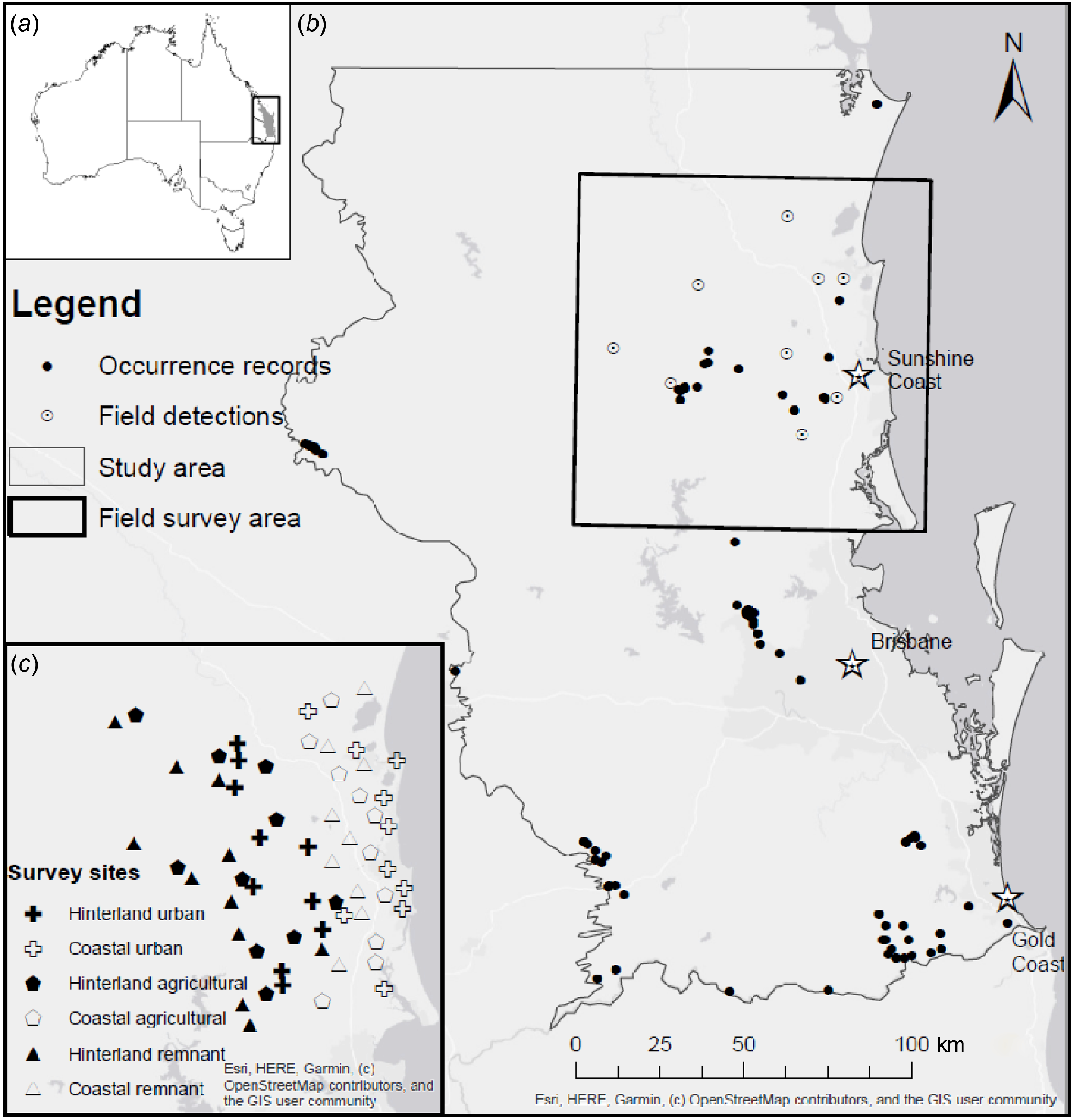
The study area covers approximately 36,000 km2, roughly encompassing the central third of the SEQ bioregion (Fig. 1b). The study area stretches from the Gold Coast area northward to Rainbow Beach and inland as far as Toowoomba and Nanango. The SEQ bioregion is Queensland’s most densely populated, containing over 70% of the state’s human population (EHP 2016). It also contains a diverse combination of landforms, soils and climate, resulting in a diversity of habitats and wildlife species (McFarland 1998).
(a) Map of Australia showing relative location of SEQ. (b) Study area containing the southern section of the SEQ Bioregion. Included are the occurrence records from which our SDM was derived and greater sooty owl (Tyto tenebricosa) detections from field surveys. (c) Field survey area in the Greater Sunshine Coast region with call playback survey sites marked.
Collating species occurrence records
We collated occurrence records of the greater sooty owl from online databases including BirdLife Australia, Atlas of Living Australia (ALA) and WildNet on 18 June 2019. These sources returned 780 raw occurrence records for which metadata fields such as record ID, location, precision and date of collection were available. Prior to modelling, records were vetted in several ways to retain only reliable and unique data for SDM development. Records collected prior to 2000 were excluded to reflect current owl habitat rather than historical owl habitat that may no longer be relevant. Records with insufficient accuracy were omitted, to ensure that our analysis included only habitat in close proximity to true owl home ranges. We deemed records with a co-ordinate uncertainty of >2.36 km to be insufficiently accurate, with this threshold being calculated as the radius of a circle encompassing an area equal to the largest recorded home range of a greater sooty owl (17.75 km2; Bilney et al. 2011a; Supplementary File S1). Duplicated records were removed, and the remaining records were manually checked. The final dataset used in SDM development contained 84 greater sooty owl occurrence points (Fig. 1b).
Species distribution model development and evaluation
This study explored eight environmental variables, selected on the basis of a priori understanding of greater sooty owl ecology (Table S1). These included three bioclimatic variables (annual mean temperature, annual precipitation and precipitation seasonality; Xu and Hutchinson 2013), elevation (QSpatial 2019a), land cover (categorical variable with five classes; Wilson et al. 2002), density of watercourses (QSpatial 2019b) and roads (QSpatial 2019c), and broad vegetation group (BVG; Neldner et al. 2017). Broad vegetation group is a categorical variable distinguishing between 22 vegetation types present in Queensland. Seven BVGs did not occur in SEQ; so, for SDM development, BVG represents a categorical variable with 15 classes (see Table S1 for full list of BVGs and the extent of each within SEQ). All variables included were considered to be either directly linked to species distribution (e.g. BVG) or surrogate measures for other features of the environment (e.g. road density is a surrogate for urbanisation). All environmental variable layers were developed and resampled to 250 m grids in ArcMap (ver. 10.6.1; ESRI 2018).
Sample selection bias in our dataset was accounted for by using a ‘target group’ background sampling approach to generate a bias layer (Phillips et al. 2009). We gathered all ALA records for nocturnal forest birds (all species within the orders Strigiformes and Caprimulgiformes) that were deemed sufficiently accurate (coordinate uncertainty included and <1000 m) across the study region. These species were selected because most survey methods to detect them would also likely detect greater sooty owls. This provides an indication of sampling intensity across the landscape (Molloy et al. 2017; Moore et al. 2019). Using these records, a bias layer was derived by conducting a point density analysis in ArcMap (ESRI 2018). The resulting layer was included as a bias file in SDM development.
Species distribution model building was performed using the Maxent software package (ver. 3.4.1; Phillips et al. 2006; Phillips and Dudík 2008). This method of machine learning correlates presence-only data to predictor variables on the basis of the maximum entropy algorithm (Merow et al. 2013) and has been widely used for research and management purposes (Radosavljevic and Anderson 2014). Most statistical machine learning and deep learning models do not handle categorical variables very well. One advantage of Maxent is that it can handle both categorical and numerical variables (Elith et al. 2011). Prior to model building, all continuous variables were tested for multicollinearity by using Spearman’s rank order correlation analysis using the Psych package (ver. 2.5.6; Revelle and Revelle 2015) in R (ver. 1.2.1335; R Core Team 2019). A threshold of r > 0.8 was considered to indicate substantial collinearity between predictors. For variables showing substantial correlation, the biological relevance of the variable and its contribution to the model based on the Maxent jackknife test results were considered and the variable judged least important was omitted. Parameters that varied in model development were the regularisation multiplier (at 0.5, 1.0, 1.5, 2.0, 2.5, 3.0, 3.5 and 4.0) and the features (using a combination of linear, quadratic and hinge). The regularisation multiplier controls model complexity by penalising overfitting; higher values produce smoother, more generalised predictions by constraining the influence of individual predictor variables (Phillips and Dudík 2008). All models were run with three-fold cross-validation to reduce overfitting (Merow et al. 2013). Ten thousand background points were randomly and automatically selected by the model from across the study area. Maxent was run with 500 iterations and by using the logistic output format, which gives habitat suitability values between 0 and 1. The resulting models were evaluated on the basis of the area under the receiver operating curve (AUC), where AUC of >0.7 indicates good discriminatory power (Hosmer and Lemesbow 1980), then externally using Akaike information criterion (AIC) values calculated using ENMtools (Warren et al. 2010). The model with the highest average training AUC and lowest AIC was determined as the most parsimonious and was used for further analysis.
A distribution map representing suitable greater sooty owl habitat under current environmental conditions was generated. This was reclassified using the 10th percentile threshold to create a binary map of predicted areas of suitable and unsuitable habitat. This process calculates the mean 10th percentile training value across cross-validated models and applies it as the threshold differentiating between suitable and unsuitable habitat. Whereas the use of thresholds has its limitations (Liu et al. 2013), many real applications of SDMs require binary outputs, and, in these instances, the 10th percentile threshold is preferred because of its conservative nature, and has been widely used in SDM studies (Bradsworth et al. 2017; Shimizu-Kimura et al. 2017).
Validation of Maxent model using field data
We undertook targeted owl surveys in a subset of the bioregion, covering approximately 8000 km2 in the Greater Sunshine Coast region (Fig. 1c). Our field survey area encompassed low-lying coastal areas, as well as mountain range and hinterland sites up to 75 km inland of the coastline. The field survey area contains significant urban areas, especially in the coastal area between Noosa Heads and Caloundra, but most of the area is made up of agricultural zones (dairy farming, cattle grazing or cropping), or is classified as parklands or environmental reserves (EHP 2016). We established 60 survey sites (Fig. 1c) stratified according to the land-use type and landscape position. Land-use types considered were remnant forest, agricultural and suburban. Landscape position distinguished between coastal (<100 m altitude) and hinterland sites (>100 m altitude). Sites were initially selected using satellite imagery where open pasture or crops were considered agricultural, large patches of continuous native forest were considered remnant and areas with a relatively high density of buildings, and lacking the above traits were considered suburban. Across all three land-use types, each site was placed adjacent to at least a few large trees in accordance with the ecology of the forest birds being surveyed, namely their use of trees as hunting perches, roosting and nesting sites. These constraints on site selection, coupled with the scarcity of coastal remnant sites within our study area, meant that one coastal remnant site was substituted for an extra hinterland remnant site. The final site breakdown was 11 hinterland remnant, 9 coastal remnant, 10 hinterland agricultural, 10 coastal agricultural, 10 hinterland suburban, and 10 coastal suburban sites.
Call playback surveys were undertaken between May and September 2019 and June and July 2020. We followed the call playback survey protocols used for forest owls in other parts of Australia (e.g. Loyn et al. 2001; Parker et al. 2007; Weaving et al. 2011; Todd et al. 2018; see Supplementary File S2 for further detail). All call playback surveys were undertaken from the roadside for consistency and practicality. To avoid double counting of owls, no sites were located within 6 km of another, in alignment with current views on the home-range area of forest owls (Kavanagh et al. 1995; Loyn et al. 2001; Soderquist and Gibbons 2007; Carter et al. 2025).
We used occupancy modelling framework to account for imperfect detection and estimate site occupancy across our 60 survey sites by using the Unmarked package in R (MacKenzie et al. 2002; Fiske and Chandler 2011). Because of the relatively few study sites (n = 60) and a high number of parameters, a global occupancy model containing all hypothesised detection (wind, temperature, moon phase, time since sunset) and occupancy (Maxent habitat suitability, BVG, land cover, watercourse density, road density, annual temperature, annual precipitation, precipitation seasonality and elevation) covariates could not be fit. Instead, we fitted all possible models, including up to four variables across both detection and occupancy submodels. For example, one model included all four detection covariates and no occupancy covariates, other models included two detection covariates and two occupancy covariates, other models included one detection covariate and one occupancy covariate, etc. The two categorical covariates, BVG and land cover, could only be included as the sole variable in the occupancy submodel because of the number of classes (n = 5 for each; surveys sites occurred within only five BVGs), leading to models failing to run if incorporated with other variables. We also included Maxent-derived habitat suitability as a sole variable in occupancy submodels because this variable was derived from a combination of the other occupancy covariates. Last, we never included annual mean temperature in the same model as elevation because these two variables were correlated (r > 0.7). This left a combination of 393 candidate models that were used for model selection. Co-efficients were reported for all models considered to have substantial support (delta AIC of <2; Burnham and Anderson 2004). We considered the Maxent model validated if Maxent-derived habitat suitability contributed to supported models, and expected a positive relationship between habitat suitability and occupancy (Law et al. 2017).
Following the method of Cooke et al. (2017), we used the constant detection model to explore the number of repeated surveys required to determine a site-specific absence at the 80%, 90% and 95% confidence levels by using the following formula:
where P is the cumulative nightly detection probability, p1 is the detection probability for Night 1 and n is the total number of survey nights.Results
Species distribution modelling
The model determined as most parsimonious performed well, with an average training AUC of 0.95 and the lowest AIC value. This model used quadratic and hinge functions and a regularisation multiplier of 1.5. No other candidate models received support (AIC < 2; see Supplementary File S3, Table S2 for model selection table). Mean annual temperature was found to be highly correlated with elevation and, so, was excluded from the modelling process. BVG (36.4%), elevation (26.8%) and annual precipitation (18.4%) contributed most to the model of the seven variables used (Table 1). The model suggests that rainforest and wet eucalypt open forest vegetation types, high rainfall and elevation provide optimal greater sooty owl habitat (Supplementary File S3).
| Variable | Relative contribution (%) | |
|---|---|---|
| Broad vegetation group | 36.4 | |
| Elevation | 26.8 | |
| Annual precipitation (Bioclim12) | 18.4 | |
| Land cover | 12.5 | |
| Road density | 4.0 | |
| Watercourse density | 1.0 | |
| Precipitation seasonality (Bioclim15) | 1.0 |
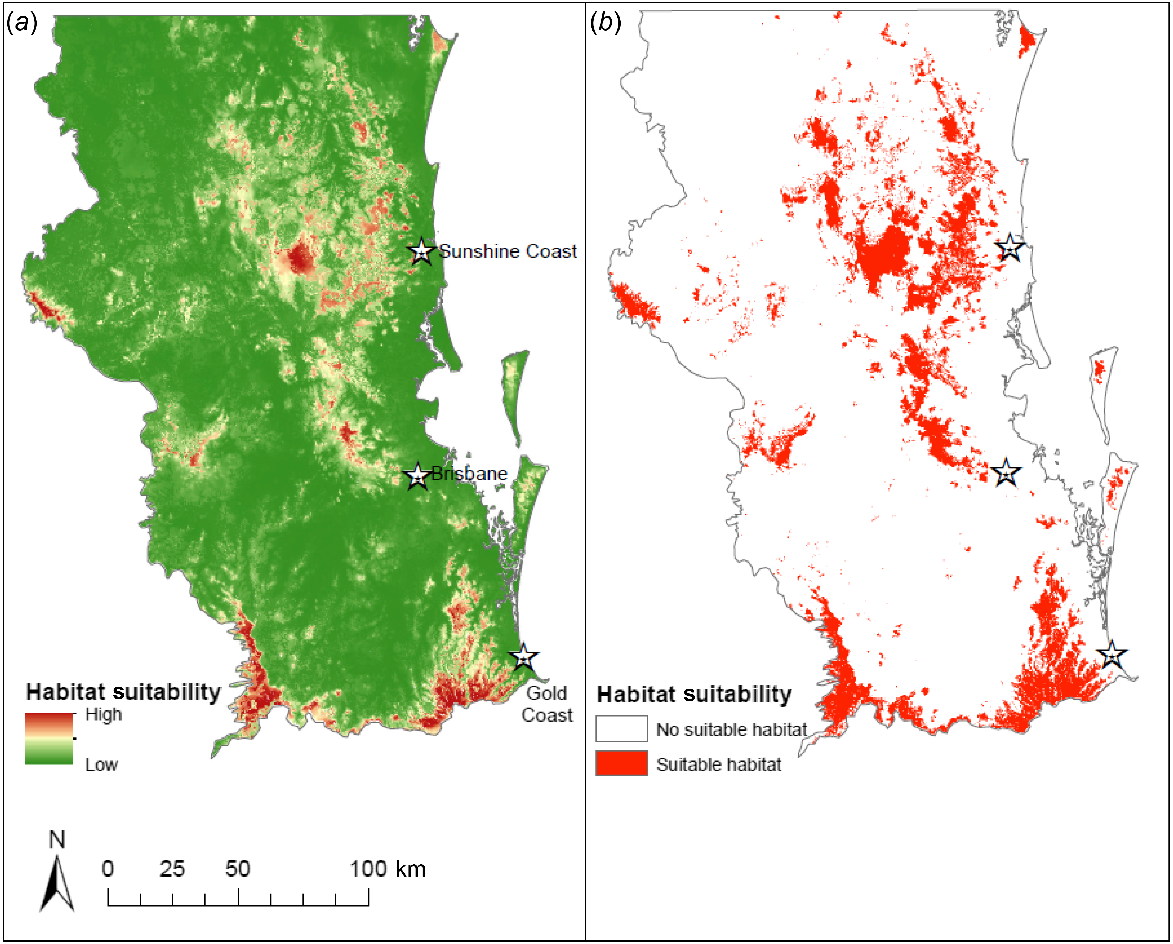
The binary map (Fig. 2b) generated by the Maxent output contains roughly 4200 km2 of suitable habitat, compared with 31,700 km2 of unsuitable habitat for greater sooty owls in SEQ (at 250 m grids) under current environmental conditions. Suitable habitat is largely restricted to areas of remnant and relatively unfragmented forest (e.g. Scenic Rim, D’Aguilar, Blackall and Conondale ranges). Approximately 42% of predicted suitable habitat for the greater sooty owl falls within protected areas, with a further 12% within the boundary of mixed-use state forests.
(a) Maxent logistic output showing predicted greater sooty owl (Tyto tenebricosa) habitat suitability across south-east Queensland, Australia. Warmer colours show areas predicted to have more suitable environmental conditions. (b) Binary map distinguishing between predicted suitable and unsuitable habitat.
Validation of Maxent model using field data
One hundred and eighty field surveys were undertaken across the 60 sites (three visits to each site), resulting in 11 detections of greater sooty owls across nine sites. Other species detected but not used in this study include Australian boobook (Ninox Boobook), barking owl (N. connivens), eastern barn owl (Tyto javanica), masked owl (T. novaehollandiae), tawny frogmouth (Podargus strigoides), marbled frogmouth (P. ocellatus), Australian owlet-nightjar (Aegotheles cristatus), and white-throated nightjar (Eurostopodus mystacalis). The powerful owl (Ninox strenua) was notably absent despite being included in call playback methodology.
Overall, greater sooty owls were detected on 6.1% of surveys, with a naïve site occupancy of 15%. Greater sooty owls were found across all three landscape types (but we note in all cases owls were located in forest patches within the larger landscape), but were more commonly detected in remnant forest sites (n = 5) than suburban (n = 3) or agricultural sites (n = 1). Detections were evenly spread between hinterland (n = 5) and coastal (n = 4) sites.
Modelling found constant detection to be among the best-supported models (Table 2), with a detection probability of 0.19 (± 0.12 s.e.), indicating that variables such as wind speed, temperature, time after sunset or moon phase had a limited effect on detectability. Other models received support (AIC < 2), including the detection covariates temperature, moon phase and time after sunset (Table 2). However, model summaries showed that in no cases did any of these variables have a significant effect on detectability (Table 3). Assuming constant detectability, to be 95% confident of site-specific absence, 14 repeated surveys were required, compared with eight repeated surveys to be 80% confident (Table 4).
| Model | AIC | Delta AIC | AIC Weight | Number of parameters | logLik | |
|---|---|---|---|---|---|---|
| ψ (Maxent)p(temp) | 79.94 | 0.00 | 0.203 | 4 | −37.88 | |
| ψ (Maxent)p(.) | 79.99 | 0.05 | 0.198 | 3 | −39.84 | |
| ψ (Maxent)p(moon) | 81.28 | 1.34 | 0.104 | 4 | −39.60 | |
| ψ (Maxent)p(moon + temp) | 81.58 | 1.64 | 0.089 | 5 | −40.18 | |
| ψ (Maxent)p(time) | 81.68 | 1.74 | 0.085 | 4 | −39.39 | |
| ψ (BVG)p(.) | 81.91 | 1.97 | 0.076 | 7 | −40.34 | |
| ψ (Maxent)p(time + temp) | 81.94 | 2.00 | 0.075 | 5 | −40.11 | |
| ψ (BVG)p(temp) | 82.14 | 2.20 | 0.067 | 4 | −39.05 |
Detection covariates shown are temperature (temp), moon phase (moon) and time after sunset (time). Occupancy covariates shown are Maxent-modelled habitat suitability (Maxent) and broad vegetation group (BVG). The eight highest-performing models according to AIC are presented.
| Variable | Estimate | s.e. | Z | P | |
|---|---|---|---|---|---|
| Intercept (ψ) | −2.34 | 0.76 | −3.10 | 0.002 | |
| Maxent | 5.49 | 2.48 | 2.22 | 0.027 | |
| Intercept (p) | 1.47 | 2.08 | 0.70 | 0.481 | |
| Temperature | −0.19 | 0.14 | −1.32 | 0.186 | |
| Intercept (ψ) | −2.18 | 0.80 | −2.71 | 0.007 | |
| Maxent | 5.27 | 2.49 | 2.12 | 0.034 | |
| Intercept (p) | −1.13 | 0.59 | −1.92 | 0.055 | |
| Intercept (ψ) | −2.27 | 0.79 | −2.89 | 0.004 | |
| Maxent | 5.07 | 2.32 | 2.19 | 0.029 | |
| Intercept (p) | −1.55 | 0.79 | −1.98 | 0.048 | |
| Moon | 0.97 | 1.18 | 0.82 | 0.414 | |
| Intercept (ψ) | −2.38 | 0.75 | −3.19 | 0.001 | |
| Maxent | 5.28 | 2.34 | 2.25 | 0.024 | |
| Intercept (p) | 1.02 | 2.27 | 0.45 | 0.653 | |
| Moon | 0.72 | 1.23 | 0.59 | 0.558 | |
| Temp | −0.18 | 0.15 | −1.20 | 0.230 | |
| Intercept (ψ) | −2.34 | 0.83 | −2.81 | 0.005 | |
| Maxent | 5.31 | 2.35 | 2.26 | 0.024 | |
| Intercept (p) | −1.64 | 1.14 | −1.43 | 0.152 | |
| Time | 0.196 | 0.41 | 0.48 | 0.634 | |
| Intercept (ψ) | 4.77 | 37.5 | 0.13 | 0.899 | |
| BVG 17 | −6.61 | 37.4 | −0.18 | 0.860 | |
| BVG 2 | −2.96 | 37.0 | −0.08 | 0.936 | |
| BVG 3 | −6.12 | 37.4 | −0.16 | 0.870 | |
| BVG 4 | −14.44 | 82.5 | −0.18 | 0.861 | |
| Intercept (p) | −1.40 | 0.64 | −2.20 | 0.028 | |
| Intercept (ψ) | −2.33 | 0.78 | −2.97 | 0.003 | |
| Maxent | 5.50 | 2.50 | 2.20 | 0.028 | |
| Intercept (p) | 1.58 | 2.71 | 0.58 | 0.561 | |
| Temp | −0.19 | 0.15 | −1.25 | 0.210 | |
| Time | −0.02 | 0.37 | −0.07 | 0.948 |
Detection (p) covariates shown are temperature (temp), moon phase (moon) and time after sunset (time). Occupancy (ψ) covariates shown are Maxent-modelled habitat suitability (Maxent) and broad vegetation group (BVG).
| Naïve ψ | Estimated ψ | P | s.e. (P) | 80% | 90% | 95% | |
|---|---|---|---|---|---|---|---|
| 0.15 | 0.31 | 0.19 | 0.116 | 8 (3–20) | 11 (4–42) | 14 (5–55) |
Values represent the naïve and estimated site occupancy (ψ), nightly detection probability (P) and standard errors (s.e. (P)), as well as the number of surveys (with 95% confidence intervals) required to have 80%, 90% and 95% confidence of a site-specific absence.
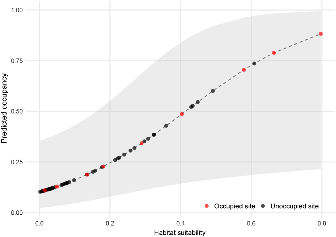
Assuming constant detection and occupancy, greater sooty owl occupancy across our survey sites was estimated to be 0.31 (±0.18). Model selection showed seven models to receive substantial support (AIC < 2), including two occupancy covariates, namely, Maxent-derived habitat suitability and broad vegetation group (Table 2). Model summaries showed that Maxent-derived habitat suitability had a significant positive effect on occupancy in all supported models in which it was included as a covariate (Table 3). Indeed, three of the four most suitable field sites according to the Maxent model, were found to be occupied by greater sooty owls during surveys (Fig. 3). Supported models including BVG as a covariate failed to show a significant relationship with occupancy (Table 3).
Discussion
We demonstrate the value of field-validated species distribution modelling to inform conservation strategies for wildlife species, using the greater sooty owl as a case study. Our species distribution model had high discriminatory power, and independent ground-truthing showed that the model was reliable in predicting potential habitat and occupancy. Our results align with other work finding that greater sooty owls prefer large areas of continuous, wet eucalypt and rainforest (Higgins 1999; Bilney et al. 2011a). Our region-wide model could be used to guide land management decisions (e.g. proposed land clearing for development or timber production) and future targeted surveys. Such models are valuable within the context of SEQ being the most populated bioregion of Queensland (EHP 2016), and also one of the most biodiverse (McFarland 1998), making simultaneous conservation and development a challenge. To our knowledge, no previous attempt has been made to model greater sooty owl distribution across SEQ. We present methods to do so using publicly available species occurrence records, spatial layers and software. Our field validation supports the accuracy of the modelling, which we recommend to be trialled for other species of conservation concern within SEQ.
The role of environmental variables in determining species distribution
The spatial relationship between species and environmental variables has become a central paradigm across multiple disciplines (Elith and Leathwick 2009; Elith et al. 2011). Interactions between species and their environment are often complex but are a crucial aspect of ecology and are necessary for conservation initiatives to be successful. Owing to the complex nature and inter-relatedness of many environmental variables, the exact relationship between species and variables is often unclear. Nevertheless, identifying broad patterns in distribution is useful.
Our habitat model predicts that, under current environmental conditions, greater sooty owls are more likely to occur in high-rainfall areas and to inhabit remnant rainforest and wet eucalypt forest (see Supplementary File S3). This aligns with other research finding that the species is most often found in wetter, more senescent forest (Higgins 1999; Loyn et al. 2001; Bilney et al. 2011a). Higher elevations and lower road densities increased the probability of suitable habitat being present, and continuous forest characterised by woody vegetation cover was by far the land cover type most likely to provide suitable habitat. This strong association with continuous areas of wet forest is likely to reflect the dietary and shelter resource requirements of the greater sooty owl. As a large predator, it requires a constant supply of food to fulfil its energetic demands. Wet forest types are among the most productive ecosystems in Australia (Roxburgh et al. 2004) and, thus, can support plentiful numbers of the small and medium-sized mammal species that comprise the greater sooty owl’s preferred prey. Greater sooty owls are more reliant on tree hollows for daytime roost sites than is sympatric powerful owl, and are rarely found roosting on an exposed branch when suitable hollows are available (Higgins 1999; L’Hotellier and Bilney 2016). Large, old-growth trees are required for formation of hollows of sufficient size for greater sooty owl roosts. Unfortunately, such trees are becoming increasingly scarce in human-modified landscapes, further restricting greater sooty owl presence to remnant forest where hollows are more available (Kavanagh 2002b).
Model performance and field validation
Recent studies have highlighted the potential for autocorrelation among testing and training data to drive high AUC values overestimating a model’s predictive ability (Ploton et al. 2020). Thus, it is important to be able to assess models externally where possible to ensure the validity of model outputs, which may be used to inform decision-making. In this study, we used field validation to assess Maxent models which, themselves, used cross-validation and the resulting AUC and AIC scores. Both forms of validation indicated that the model had good discriminatory ability. The high AUC value of 0.95 was supported by field validation where occupancy (adjusted for imperfect detectability) rose in a linear fashion as Maxent-derived habitat suitability values increased. This linear relationship shows that greater sooty owls are, in fact, occupying areas that our model predicted as good habitat. While greater sooty owls were detected in some sites that were predicted to be ‘poor’ habitat, the majority of poor sites returned no detections. Greater sooty owls were detected at only one of the 20 lowest-ranked sites, compared with three of the four top-ranked sites. Species distribution models are known to be highly variable depending on inputs and, so, the additional measure of field validation adds merit to the accuracy of our model in predicting suitable greater sooty owl habitat (Law et al. 2017; Finn et al. 2024).
The Maxent-modelled habitat suitability values showed a significant positive relationship with occupancy and were included as a co-variate in five of seven occupancy models with substantial support (delta AIC < 2). The other supported model incorporated BVG, but this variable failed to show a significant relationship with occupancy. Thus, we conclude that Maxent model-derived habitat suitability values outperformed other variables in predicting greater sooty owl occupancy at our field sites. This is consistent with the view that there are multiple determinants of owl habitat (Bilney et al. 2011a) because habitat suitability values that incorporated a range of features such as vegetation type, climate, topographic position and types of human land-use present, performed best in predicting greater sooty owl habitat. Although the Maxent model developed here performed well, discriminatory ability could be further enhanced through the development and inclusion of additional GIS layers for environmental variables relevant to greater sooty owl ecology such as tree hollow indices, prey abundance, forest age and fire history, which were not available to us.
Maxent model uncertainties and data biases
In this study, SDM provided a useful tool to evaluate general trends in habitat distribution for our study species. However, not encompassed within the final model is the uncertainty involved in model and variable selection (Beale and Lennon 2012). Lack of region-wide environmental variable layers relevant to owl distribution such as hollow indices and forest age were a limitation to model development. Additionally, presence-only modelling, such as used here (cf. presence–absence modelling), has a general tendency to overestimate the spatial extent of distributions (Brotons et al. 2004). However, presence-only modelling does provide a viable alternative where datasets are incomplete and/or absence difficult to determine, as in the case of our study.
Our occurrence record database was composed of biodiversity atlas records contributed by the public and, thus, exposed to spatial, detectability and taxonomic reporting biases (Bonney et al. 2009; Geldmann et al. 2016). During this study, we found it difficult to determine spatial accuracy of occurrence records, especially when compiling records across several data sources and where different data vetting processes may or may not have been undertaken. Even with thorough vetting, citizen science data have inherent risks of misidentification and other human error but have been shown to be a useful tool for ecological study here and elsewhere (Bradsworth et al. 2017; Matutini et al. 2021; Pyne et al. 2024). As a large, charismatic species, greater sooty owls attract public interest, leading to relatively extensive citizen science datasets. For smaller, lesser-known species (e.g. some species of rodent or skink), occurrence data across their range are often scarce and patchy, which may lead to contrasting results of broad-scale modelling (e.g. SDMs) and fine-scale modelling based on field surveys. Thus, the approach demonstrated here may be best suited for species with ample occurrence records available.
Estimating detectability from field surveys
The modelled single-visit detection probability of 0.19 was similar to other estimates for this species (Debus 1995; Wintle et al. 2005), but varied substantially from other estimates (P = 0.4; Kavanagh 1997). The area studied by Kavanagh (1997) is likely to have contained a higher density of greater sooty owls than in our mixed-use landscape, which may increase detection probability (Wintle et al. 2005). Fulton et al. (2020) reported a detection probability of 0.67 at one site visited 12 times over a year. This seemingly high result could have been due to the survey site being located in close proximity to core habitat such as roosting and/or nesting hollows. Additionally, this study surveyed for 2 h each visit (Fulton et al. 2020), substantially more survey time than most multi-site survey methodologies. With such a small sample size, this result should be treated cautiously but could indicate that greater sooty owls may be more detectable than initially thought, where they are present. At two of our survey sites (GCR and HHU), greater sooty owls were detected on two of three visits, somewhat supporting this notion. Nevertheless, this study reports low detectability in line with the predominantly held view that greater sooty owls are typically cryptic and difficult to detect during brief surveys, such as employed by the present and most other surveys (Wintle et al. 2005; Cooke et al. 2017; Cisterne et al. 2020).
Constant detection was among the most supported models during our analysis, indicating that neither wind speed, temperature, moon phase or time after sunset had a significant effect on detectability. Wintle et al. (2005) showed similar findings but found temperature to have a positive relationship with greater sooty owl detectability. This relationship has also been observed in other Australian large forest owls, such as masked (Todd et al. 2018) and powerful owls (Cooke et al. 2017). However, these studies were conducted in cooler climates where nightly temperatures drop considerably lower than in our subtropical study area. Wind has been recorded to negatively influence owl detection (Todd et al. 2018). This effect was assumed in our study design, leading to survey abandonment where local wind speeds were forecast to exceed 20 km/h. Thus, although included in our models, the effect of wind speed on detection was not truly explored here.
Management implications and recommendations
Currently, greater sooty owls are not threatened nationally or within Queensland but are threatened in New South Wales and Victoria, the other two states they occupy. Owing to their cryptic nature and lack of survey effort, greater sooty owl and other forest owl species population metrics are not well-known, and these species are at a comparatively high risk of extinction because of their position as apex predators and reliance on large tracts of intact forest (McGregor 2011). This is especially pertinent when placed in the context of increasingly frequent large-scale disturbances in Australia, such as fire and land clearing (Reside et al. 2017; Nimmo et al. 2021). Therefore, identification and conservation of forest owl habitat is of crucial importance.
Under the current reserve system, a significant amount (42%) of predicted greater sooty owl habitat within SEQ is protected. We have identified relatively large, continuous tracts of suitable habitat across Main Range, D’Aguilar, Lamington and Conondale national parks. Therefore, we posit that these areas are of particular importance for greater sooty owl conservation in SEQ. However, this does leave the majority of suitable habitat within private land or mixed-use state forest, exposing large amounts of owl habitat to anthropogenic impacts. To protect such habitat, we recommend further work into the identification and protection of greater sooty owl habitat. Valuable foraging areas may be difficult to determine, but roost and nest sites are typically obvious once they are located (identified by extensive whitewash and pellets containing prey remains). Greater sooty owls show high fidelity at these sites even through generations (Fleay 1972; Bilney 2015), with such sites being considered to be of major importance in owl ecology (McNabb et al. 2003; Isaac et al. 2014; McDonald et al. 2014). Therefore, identifying roosting and nesting sites presents as an important target for the conservation research of these species, and could incorporate emerging technologies (e.g. drones, thermal sensors, etc.) to maximise effectiveness (Murphy et al. 2024). Furthermore, we recommend combining SDMs with GPS-tracking studies (e.g. Bradsworth et al. 2017; Carter et al. 2019) for our study species, to gain fine-scale data of greater sooty owl movements within the landscape.
We suggest the establishment of protective buffer zones around important owl sites (roosts and nests) on crown land in SEQ, as has been implemented in Victorian forestry areas (Bilney et al. 2011a). We encourage local governments to participate in community initiatives, such as the Powerful Owl Project (Bain et al. 2014), to engage and educate landowners of how they can assist in owl conservation. Furthermore, we recommend ongoing surveys into the future to monitor known populations and identify new territories. Our habitat modelling has identified the following high-priority survey areas containing potential greater sooty owl habitat with few or no recent records of occurrence: Ravensbourne National Park (NP), Wrattens NP and State Forest (SF), Yabba SF, Imbil SF, Deongwar SF, and Diaper SF. Habitat modelling may also be useful to guide pre-clearance surveys prior to habitat destruction, which occurs to facilitate urban and agricultural expansion. We suggest that areas of predicted suitable habitat should be surveyed for greater sooty owls at least eight times prior to land clearing, to achieve 80% certainty of absence (on the basis of constant detection probability of 0.19 in our study). We encourage further survey on private land surrounding areas of high suitability we have identified here.
Whereas small-scale, site-specific variables undoubtedly play a role in habitat selection, these data are often labour-intensive and expensive to collect. Future studies might combine field habitat variables such as number of hollow-bearing trees and floristic composition with landscape-level variables (e.g. Loyn et al. 2001) over a subset of our study area. Our study used only freely available software, occurrence records and spatial data resulting in a methodology that can realistically be employed by land managers. Field validation supports the accuracy of our species distribution modelling, highlighting the utility of the method in identifying habitat, which can be applied to a suite of species of conservation concern.
Declaration of funding
Funding was provided by the University of the Sunshine Coast, the Friends of Mary Cairncross and the Environmental Legacy Foundation.
Acknowledgements
We pay respects to the Gubbi Gubbi and Waka Waka peoples, traditional custodians of the lands on which fieldwork for this project was conducted. We thank Anna Aristova and Riley Logan for their assistance with fieldwork. We are grateful to Sanjeev Srivastava for providing technical support with Geographic Information Systems.
References
Ball IR, Lindenmayer DB, Possingham HP (1999) A tree hollow dynamics simulation model. Forest Ecology and Management 123, 179-194.
| Crossref | Google Scholar |
Beale CM, Lennon JJ (2012) Incorporating uncertainty in predictive species distribution modelling. Philosophical Transactions of the Royal Society B: Biological Sciences 367, 247-258.
| Crossref | Google Scholar |
Bilney R (2015) What sooty owls used to eat: a history of mammal losses in eastern Victoria. Wildlife Australia 52, 28-31.
| Google Scholar |
Bilney RJ, Bilney RJ (2015) The diet of a masked owl from a sub-alpine roost. Victorian Naturalist 132, 88-89.
| Google Scholar |
Bilney RJ, Cooke R, White J (2006) Change in the diet of sooty owls (Tyto tenebricosa) since European settlement: from terrestrial to arboreal prey and increased overlap with powerful owls. Wildlife Research 33, 17-24.
| Crossref | Google Scholar |
Bilney RJ, Kavanagh RP, Harris JM (2007) Further observations on the diet of the sooty owl Tyto tenebricosa in the Royal National Park, Sydney. Australian Field Ornithology 24, 64-69.
| Google Scholar |
Bilney RJ, White JG, L’Hotellier FA, Cooke R (2011a) Spatial ecology of sooty owls in south-eastern Australian coastal forests: implications for forest management and reserve design. Emu - Austral Ornithology 111, 92-99.
| Crossref | Google Scholar |
Bilney RJ, White JG, Cooke R (2011b) Reversed sexual dimorphism and altered prey base: the effect on sooty owl (Tyto tenebricosa tenebricosa) diet. Australian Journal of Zoology 59, 302-311.
| Crossref | Google Scholar |
Bonney R, Cooper CB, Dickinson J, Kelling S, Phillips T, Rosenberg KV, Shirk J (2009) Citizen science: a developing tool for expanding science knowledge and scientific literacy. BioScience 59, 977-984.
| Crossref | Google Scholar |
Bradsworth N, White JG, Isaac B, Cooke R (2017) Species distribution models derived from citizen science data predict the fine scale movements of owls in an urbanizing landscape. Biological Conservation 213, 27-35.
| Crossref | Google Scholar |
Brotons L, Thuiller W, Araújo MB, Hirzel AH (2004) Presence–absence versus presence-only modelling methods for predicting bird habitat suitability. Ecography 27, 437-448.
| Crossref | Google Scholar |
Burnham KP, Anderson DR (2004) Multimodel inference: understanding AIC and BIC in model selection. Sociological Methods & Research 33, 261-304.
| Crossref | Google Scholar |
Carter N, Cooke R, White JG, Whisson DA, Isaac B, Bradsworth N (2019) Joining the dots: how does an apex predator move through an urbanizing landscape? Global Ecology and Conservation 17, e00532.
| Crossref | Google Scholar |
Carter N, White JG, Bridgeman W, Bradsworth N, Ross TA, Cooke R (2025) Where to fly? Landscape influences on the movement and spatial ecology of a threatened apex predator. Landscape and Urban Planning 253, 105218.
| Crossref | Google Scholar |
Cisterne A, Crates R, Bell P, Heinsohn R, Stojanovic D (2020) Occupancy patterns of an apex avian predator across a forest landscape. Austral Ecology 45, 825-833.
| Crossref | Google Scholar |
Cooke R, Wallis R, Hogan F, White J, Webster A (2006) The diet of powerful owls (Ninox strenua) and prey availability in a continuum of habitats from disturbed urban fringe to protected forest environments in south-eastern Australia. Wildlife Research 33, 199-206.
| Crossref | Google Scholar |
Cooke R, Grant H, Ebsworth I, Rendall AR, Isaac B, White JG (2017) Can owls be used to monitor the impacts of urbanisation? A cautionary tale of variable detection. Wildlife Research 44, 573-581.
| Crossref | Google Scholar |
de Thoisy B, Fayad I, Clément L, Barrioz S, Poirier E, Gond V (2016) Predators, prey and habitat structure: can key conservation areas and early signs of population collapse be detected in neotropical forests? PLoS ONE 11, e0165362.
| Crossref | Google Scholar |
Debus SJS (1995) Surveys of large forest owls in northern New South Wales: methodology, calling behaviour and owl responses. Corella 19, 38-50.
| Google Scholar |
Elith J, Leathwick JR (2009) Species distribution models: ecological explanation and prediction across space and time. Annual Review of Ecology, Evolution, and Systematics 40, 677-697.
| Crossref | Google Scholar |
Elith J, Phillips SJ, Hastie T, Dudík M, Chee YE, Yates CJ (2011) A statistical explanation of MaxEnt for ecologists. Diversity and Distributions 17, 43-57.
| Crossref | Google Scholar |
ESRI (2018) ArcMap version 10.6. 1. Environmental Systems Research Institute Redlands, CA, USA. https://desktop.arcgis.com/en/arcmap/latest/get-started/main/get-started-with-arcmap.htm
Finn KJ, Bergman JC, Lee-Yaw JA (2024) Deciding where to put them: sensitivity tests and independent evaluation are critical when using species distribution models to inform conservation translocations. Journal of Applied Ecology 61, 713-732.
| Crossref | Google Scholar |
Fiske I, Chandler R (2011) Unmarked: an R package for fitting hierarchical models of wildlife occurrence and abundance. Journal of Statistical Software 43, 1-23.
| Crossref | Google Scholar |
Franklin AB, Anderson DR, Gutiérrez RJ, Burnham KP (2000) Climate, habitat quality, and fitness in Northern Spotted Owl populations in northwestern California. Ecological Monographs 70, 539-590.
| Crossref | Google Scholar |
Fulton GR, Fulton GR, Cheung YW (2020) A comparison of urban and peri-urban/hinterland nocturnal birds at Brisbane, Australia. Pacific Conservation Biology 26, 239-248.
| Crossref | Google Scholar |
Geldmann J, Heilmann-Clausen J, Holm TE, Levinsky I, Markussen B, Olsen K, Rahbek C, Tøttrup AP (2016) What determines spatial bias in citizen science? Exploring four recording schemes with different proficiency requirements. Diversity and Distributions 22, 1139-1149.
| Crossref | Google Scholar |
Girini JM, Palacio FX, Zelaya PV (2017) Predictive modeling for allopatric Strix (Strigiformes: Strigidae) owls in South America: determinants of their distributions and ecological niche-based processes. Journal of Field Ornithology 88, 1-15.
| Crossref | Google Scholar |
Hosmer DW, Lemesbow S (1980) Goodness of fit tests for the multiple logistic regression model. Communications in Statistics-Theory and Methods 9, 1043-1069.
| Crossref | Google Scholar |
Huettmann F, Andrews P, Steiner M, Das AK, Philip J, Mi C, Bryans N, Barker B (2024) A super SDM (species distribution model) ‘in the cloud’ for better habitat-association inference with a ‘big data’ application of the Great Gray Owl for Alaska. Scientific Reports 14, 7213.
| Crossref | Google Scholar |
Isaac B, White J, Ierodiaconou D, Cooke R (2013) Response of a cryptic apex predator to a complete urban to forest gradient. Wildlife Research 40, 427-436.
| Crossref | Google Scholar |
Isaac B, White J, Ierodiaconou D, Cooke R (2014) Urban to forest gradients: suitability for hollow bearing trees and implications for obligate hollow nesters. Austral Ecology 39, 963-972.
| Crossref | Google Scholar |
Jensen RA, Sunde P, Nachman G (2012) Predicting the distribution of tawny owl (Strix aluco) at the scale of individual territories in Denmark. Journal of Ornithology 153, 677-689.
| Crossref | Google Scholar |
Kang T-H, Kim D-H, Lee H, Cho H-J, Hur W-H, Han S-H, Kim Y-J, Paek W-K, Jin S-D, Paik I-H (2013) Analysis of home range of Eurasian eagle owl (Bubo bubo) by WT-100. Journal of Asia–Pacific Biodiversity 6, 369-373.
| Crossref | Google Scholar |
Kavanagh RP (2002a) Comparative diets of the powerful owl (Ninox strenua), sooty owl (Tyto tenebricosa) and masked owl (Tyto novaehollandiae) in southeastern Australia. In ‘Ecology and conservation of owls’. (Eds I Newton, R Kavanagh, J Olsen, I Taylor) pp. 175–191. (CSIRO Publishing: Melbourne, Vic, Australia)
Kavanagh RP, Debus S, Tweedie T, Webster R (1995) Distribution of nocturnal forest birds and mammals in North-Eastern New South Wales: relationships with environmental variables and management history. Wildlife Research 22, 359-377.
| Crossref | Google Scholar |
Koch AJ, Munks SA, Driscoll D, Kirkpatrick JB (2008) Does hollow occurrence vary with forest type? A case study in wet and dry Eucalyptus obliqua forest. Forest Ecology and Management 255, 3938-3951.
| Crossref | Google Scholar |
Kremen C, Cameron A, Moilanen A, Phillips SJ, Thomas CD, Beentje H, Dransfield J, Fisher BL, Glaw F, Good TC, Harper GJ, Hijmans RJ, Lees DC, Louis E, Jr., Nussbaum RA, Raxworthy CJ, Razafimpahanana A, Schatz GE, Vences M, Vieites DR, Wright PC, Zjhra ML (2008) Aligning conservation priorities across taxa in Madagascar with high-resolution planning tools. Science 320, 222-226.
| Crossref | Google Scholar | PubMed |
Law B, Caccamo G, Roe P, Truskinger A, Brassil T, Gonsalves L, Mcconville A, Stanton M (2017) Development and field validation of a regional, management-scale habitat model: a koala Phascolarctos cinereus case study. Ecology and Evolution 7, 7475-7489.
| Crossref | Google Scholar | PubMed |
Lepers E, Lambin EF, Janetos AC, DeFries R, Achard F, Ramankutty N, Scholes RJ (2005) A synthesis of information on rapid land-cover change for the period 1981–2000. BioScience 55, 115-124.
| Crossref | Google Scholar |
Liu C, White M, Newell G (2013) Selecting thresholds for the prediction of species occurrence with presence-only data. Journal of Biogeography 40, 778-789.
| Crossref | Google Scholar |
Loyn RH, McNabb EG, Volodina L, Willig R (2001) Modelling landscape distributions of large forest owls as applied to managing forests in north-east Victoria, Australia. Biological Conservation 97, 361-376.
| Crossref | Google Scholar |
L’Hotellier F, Bilney R (2016) The diet and roosting sites of sooty owls Tyto tenebricosa from coastal habitats at Cape Conran, Victoria. The Victorian Naturalist 133, 46-50.
| Google Scholar |
Mackenzie DI, Nichols JD, Lachman GB, Droege S, Andrew Royle J, Langtimm CA (2002) Estimating site occupancy rates when detection probabilities are less than one. Ecology 83, 2248-2255.
| Crossref | Google Scholar |
Matutini F, Baudry J, Pain G, Sineau M, Pithon J (2021) How citizen science could improve species distribution models and their independent assessment. Ecology and Evolution 11, 3028-3039.
| Crossref | Google Scholar | PubMed |
McDonald K, Burnett S, Robinson W (2014) Utility of owl pellets for monitoring threatened mammal communities: an Australian case study. Wildlife Research 40, 685-697.
| Crossref | Google Scholar |
McGregor H (2011) Large forest owls in the river red gum state forests of south-western New South Wales-an account of their 2008 status. Australian Zoologist 35, 864-869.
| Crossref | Google Scholar |
McNabb E, McNabb J, Barker K (2003) Post-nesting home range, habitat use and diet of a female masked owl Tyto novaehollandiae in western Victoria. Corella 27, 109-117.
| Google Scholar |
Merow C, Smith MJ, Silander JA, Jr (2013) A practical guide to MaxEnt for modeling species’ distributions: what it does, and why inputs and settings matter. Ecography 36, 1058-1069.
| Crossref | Google Scholar |
Molloy SW, Davis RA, Dunlop JA, van Etten EJB (2017) Applying surrogate species presences to correct sample bias in species distribution models: a case study using the Pilbara population of the Northern Quoll. Nature Conservation 18, 27-46.
| Crossref | Google Scholar |
Moore HA, Dunlop JA, Valentine LE, Woinarski JCZ, Ritchie EG, Watson DM, Nimmo DG (2019) Topographic ruggedness and rainfall mediate geographic range contraction of a threatened marsupial predator. Diversity and Distributions 25, 1818-1831.
| Crossref | Google Scholar |
Murphy NK, Elmore JA, Boudreau MR, Dorr BS, Rush SA (2024) Monitoring active osprey nests with drones is more time efficient and less disturbing than conventional methods. Wildlife Biology e01341.
| Crossref | Google Scholar |
Nimmo DG, Carthey AJR, Jolly CJ, Blumstein DT (2021) Welcome to the Pyrocene: animal survival in the age of megafire. Global Change Biology 27(22), 5684-5693.
| Crossref | Google Scholar | PubMed |
Parker D, Webster R, Belcher C, Leslie D (2007) A survey of large forest owls in State Forests of south-western New South Wales, Australia. Australian Zoologist 34, 78-84.
| Crossref | Google Scholar |
Phillips SJ, Dudík M (2008) Modeling of species distributions with Maxent: new extensions and a comprehensive evaluation. Ecography 31, 161-175.
| Crossref | Google Scholar |
Phillips SJ, Anderson RP, Schapire RE (2006) Maximum entropy modeling of species geographic distributions. Ecological Modelling 190, 231-259.
| Crossref | Google Scholar |
Phillips SJ, Dudík M, Elith J, Graham CH, Lehmann A, Leathwick J, Ferrier S (2009) Sample selection bias and presence-only distribution models: implications for background and pseudo-absence data. Ecological Applications 19, 181-197.
| Crossref | Google Scholar | PubMed |
Ploton P, Mortier F, Réjou-Méchain M, Barbier N, Picard N, Rossi V, Dormann C, Cornu G, Viennois G, Bayol N, Lyapustin A, Gourlet-Fleury S, Pélissier R (2020) Spatial validation reveals poor predictive performance of large-scale ecological mapping models. Nature Communications 11, 4540.
| Crossref | Google Scholar |
Pyne T, Haering R, Sriram A, Lorigan S, Shine R, Jolly CJ (2024) Interactions between reptiles and people: a perspective from wildlife rehabilitation records. Royal Society Open Science 11, 240512.
| Crossref | Google Scholar |
QSpatial (2019a) Digital elevation model – 3 second – Queensland. Available at http://qldspatial.information.qld.gov.au/catalogue/
QSpatial (2019b) Watercourse lines – North East Coast drainage division. Available at http://qldspatial.information.qld.gov.au/catalogue/
QSpatial (2019c) Queensland roads and tracks. Available at http://qldspatial.information.qld.gov.au/catalogue/
R Core Team (2019) ‘R: a language and environment for statistical computing.’ (R Foundation for Statistical Computing: Vienna, Austria) Available at https://www.r-project.org/
Radosavljevic A, Anderson RP (2014) Making better MAXENT models of species distributions: complexity, overfitting and evaluation. Journal of Biogeography 41, 629-643.
| Crossref | Google Scholar |
Reside AE, Beher J, Cosgrove AJ, Evans MC, Seabrook L, Silcock JL, Wenger AS, Maron M (2017) Ecological consequences of land clearing and policy reform in Queensland. Pacific Conservation Biology 23, 219-230.
| Crossref | Google Scholar |
Revelle W, Revelle MW (2015) Package psych. The Comprehensive R Archive Network 337(338), 161-165 Available at https://cran.r-project.org/web/packages/psych/index.html.
| Google Scholar |
Ritchie EG, Johnson CN (2009) Predator interactions, mesopredator release and biodiversity conservation. Ecology Letters 12, 982-998.
| Crossref | Google Scholar | PubMed |
Rodríguez JP, Brotons L, Bustamante J, Seoane J (2007) The application of predictive modelling of species distribution to biodiversity conservation. Diversity and Distributions 243-251.
| Crossref | Google Scholar |
Roxburgh SH, Barrett DJ, Berry SL, Carter JO, Davies ID, Gifford RM, Kirschbaum MUF, McBeth BP, Noble IR, Parton WG, Raupach MR, Roderick ML (2004) A critical overview of model estimates of net primary productivity for the Australian continent. Functional Plant Biology 31, 1043-1059.
| Crossref | Google Scholar | PubMed |
Shimizu-Kimura Y, Accad A, Shapcott A (2017) The relationship between climate change and the endangered rainforest shrub Triunia robusta (Proteaceae) endemic to southeast Queensland, Australia. Scientific Reports 7, 46399.
| Crossref | Google Scholar |
Soderquist T, Gibbons D (2007) Home-range of the powerful owl (Ninox strenua) in dry sclerophyll forest. Emu - Austral Ornithology 107, 177-184.
| Crossref | Google Scholar |
Thomas CD (2011) Translocation of species, climate change, and the end of trying to recreate past ecological communities. Trends in Ecology & Evolution 26, 216-221.
| Crossref | Google Scholar | PubMed |
Thuiller W, Richardson DM, Pyšek P, Midgley GF, Hughes GO, Rouget M (2005) Niche-based modelling as a tool for predicting the risk of alien plant invasions at a global scale. Global Change Biology 11, 2234-2250.
| Crossref | Google Scholar | PubMed |
Todd MK, Kavanagh RP, Penman TD, Bell P, Munks SA (2018) The relationship between environmental variables, detection probability and site occupancy by Tasmanian nocturnal birds, including the Tasmanian masked owl (Tyto novaehollandiae castanops). Australian Journal of Zoology 66, 139-151.
| Crossref | Google Scholar |
Vanderwal J, Shoo LP, Graham C, Williams SE (2009) Selecting pseudo-absence data for presence-only distribution modeling: how far should you stray from what you know? Ecological Modelling 220, 589-594.
| Crossref | Google Scholar |
Wang Y, Allen ML, Wilmers CC (2015) Mesopredator spatial and temporal responses to large predators and human development in the Santa Cruz Mountains of California. Biological Conservation 190, 23-33.
| Crossref | Google Scholar |
Warren DL, Glor RE, Turelli M (2010) ENMTools: a toolbox for comparative studies of environmental niche models. Ecography 33, 607-611.
| Crossref | Google Scholar |
Weaving MJ, White JG, Isaac B, Cooke R (2011) The distribution of three nocturnal bird species across a suburban-forest gradient. Emu - Austral Ornithology 111, 52-58.
| Crossref | Google Scholar |
Webster A, Cooke R, Jameson G, Wallis R (1999) Diet, roosts and breeding of Powerful Owls Ninox strenua in a disturbed, urban environment: a case for cannibalism? Or a case of infanticide? Emu - Austral Ornithology 99, 80-83.
| Crossref | Google Scholar |
Wilson BA, Neldner VJ, Accad A (2002) The extent and status of remnant vegetation in Queensland and its implications for statewide vegetation management and legislation. The Rangeland Journal 24, 6-35.
| Crossref | Google Scholar |
Wintle BA, Kavanagh RP, McCarthy MA, Burgman MA (2005) Estimating and dealing with detectability in occupancy surveys for forest owls and arboreal marsupials. The Journal of Wildlife Management 69, 905-917.
| Crossref | Google Scholar |
Xu T, Hutchinson MF (2013) New developments and applications in the ANUCLIM spatial climatic and bioclimatic modelling package. Environmental Modelling & Software 40, 267-279.
| Crossref | Google Scholar |