

The Trip to the Density Functional Theory Zoo Continues: Making a Case for Time-Dependent Double Hybrids for Excited-State Problems*
Lars Goerigk A B and Marcos Casanova-Paéz A
A School of Chemistry, The University of Melbourne, Parkville, Vic. 3010, Australia.
B Corresponding author. Email: lars.goerigk@unimelb.edu.au
Australian Journal of Chemistry 74(1) 3-15 https://doi.org/10.1071/CH20093
Submitted: 19 March 2020 Accepted: 1 May 2020 Published: 30 June 2020
Abstract
This account is written for general users of time-dependent density functional theory (TD-DFT) methods as well as chemists who are unfamiliar with the field. It includes a brief overview of conventional TD-DFT approaches and recommendations for applications to organic molecules based on our own experience. The main emphasis of this work, however, lies in providing the first in-depth review of time-dependent double-hybrid density functionals. They were first established in 2007 with very promising follow-up studies in the subsequent four years before developments or applications became scarce. The topic has regained more interest since 2017, and this account reviews those latest developments led by our group. These developments have shown unprecedented robustness for a variety of different types of electronic excitations when compared to more conventional TD-DFT methods. In particular, time-dependent double hybrids do not suffer from artificial ghost states and are able to reproduce exciton-coupled absorption spectra. Our latest methods include range separation and belong to the currently best TD-DFT methods for singlet-singlet excitations in organic molecules. While there is still room for improvement and further development in this space, we hope that this account encourages users to adjust their computational protocols to such new methods to provide more real-life testing and scenarios.
Introduction
Density functional theory[1,2] (DFT) is undoubtedly the most important methodology in computational chemistry and not only used by theoreticians but also by experimentalists to shed light into chemical phenomena and problems. Its founding theorems introduced by Hohenberg and Kohn in 1964[1] are, however, only valid for electronic ground-state problems. The equivalent of the Hohenberg-Kohn theorems for excited states was formulated by Runge and Gross in 1984,[3] which marked the inception of time-dependent DFT (TD-DFT). After inclusion of additional approximations and under consideration of the interaction of electronic structures with relatively weak electromagnetic-fields,[4,5] linear-response TD-DFT has become equally important to chemists working on electronically excited-state problems as conventional DFT has become the method of choice for electronic ground states.
Any TD-DFT treatment is preceded by a ground-state calculation, and therefore both DFT ‘flavours’ share a common denominator, namely the underlying density functional approximation (DFA) to the unknown ‘true’ functional, which would solve the Schrödinger Equation exactly at a negligible cost compared to electron-correlation wave-function theory (WFT). Similar to ground-state DFT, TD-DFT algorithms are easily accessible to users through distribution in every standard quantum-chemical code. However, while that accessibility allows routine (TD-)DFT treatments, there is a risk that users may assume that such calculations can be carried out in a black-box fashion. The main reason is that the value of the insights we can gain from every calculation rises and falls with the underlying DFA; unfortunately, a plethora of DFAs have been developed and the list is growing. This leads to uncertainties in the user community, misconceptions, and the tendency to stick to popular, but outdated and unreliable DFAs. In 2019, some from our group reviewed this issue for ground-state DFT in an account in this very same journal that addressed a general readership and reported our main findings for thermochemistry, kinetics, non-covalent interactions, and geometry optimisations.[6] We ruled out common misconceptions, demonstrated that there was no correlation between the popularity of a DFA and its reliability, and gave recommendations on robust methods that enable getting the right answer for the right reason.
This present account is written in the same spirit as the one from 2019 and focusses on TD-DFT applications. We address common DFAs that constitute the large bulk of currently applied methods used in routine TD-DFT calculations, mention some common pitfalls in this area, and then focus on our own recent developments[7,8] in the field of time-dependent double-hybrid[9] DFAs (TD-DHDFAs), which alleviate some of the problems of the more widespread methods. This is not a detailed review of the underlying theory of TD-DFT and we refer the reader to more detailed papers.[4,10–15] Instead, we will discuss the relevant theories with relatively basic equations that provide a general readership and potential users of TD-DFT methods enough background knowledge without slowing down the flow of our elaborations. We start our discussion with a brief introduction to the Jacob’s Ladder scheme of DFT, an overview of TD-DFT, and common problems of the first four rungs on that ladder with recommendations based on our own experience. We then elaborate on the highest rung of Jacob’s Ladder and discuss in depth what DHDFAs are, how they have been transferred to the excited-state concept, and what their main advantages are. This is an active research field and we conclude with a list of open questions that still need to be answered. Note that most of our discussions will be limited to applications to organic molecules. However, the recommendations of this account should still be applicable to a large number of commonly conducted calculations.
The First Four Rungs on DFT’s Jacob’s Ladder
From the Local Density to the Hybrid Approximation
The first step in the treatment of electronic excited states is to establish the electronic structure of the ground state. The resulting molecular orbitals (MOs) and their energies are then used as an input for accessing higher-lying states. In the case of DFT, the electronic ground-state is established with the help of self-consistent-field (SCF) Kohn-Sham (KS) DFT[2] for which the label DFT without the prefix ‘KS’ is commonly used as a synonym; for the difference between KS-DFT and orbital-free, ‘pure’ DFT, see common textbooks.[16,17] In KS-DFT, the total electronic-energy functional is separated into four different components: the electronic kinetic energy, the attractive electron-nucleus interaction energy, the classical Coulomb electron-electron repulsion, and the exchange-correlation (XC) energy functionals. The first term calculates the kinetic energy for a fictitious reference system of non-interacting electrons that maintains the density of the real system. The second term is known exactly, while the classical Coulomb term is known but introduces the spurious interaction of an electron with itself—see Refs [18–22] for recent discussions on the yet unsolved self-interaction error (SIE). The requirements for the fourth term are to account for the SIE and any inaccuracies in the kinetic-energy expression while simultaneously introducing non-classical electron-electron exchange and correlation effects. KS-DFT is formally an exact theory, but in practice the XC functional is unknown and needs to be approximated. Conventional DFAs have therefore the first three terms in common, but differ in their expressions for exchange and correlation.
Each DFA has its own disadvantages and—to a varying degree—advantages. As a systematic improvement of DFAs is hard to achieve, DFA development is often based on a trial-and-error approach with an important benchmarking step at the end to assess the accuracy of the newly implemented approximations. The more comprehensive such studies are, the easier it is to make recommendations as to the reliability and robustness of a DFA, where the latter implies that a method can be safely used for different properties or molecule classes with roughly a similar error bar; see our recent account[6] that summarises our own contributions to comprehensive ground-state benchmarking as well as comparable studies or more recent works based upon our previous contributions.[23–27]
DFA development follows two different philosophies in which method-inherent parameters are either derived from first-principles or by fitting them to a training set of thermochemical or other data. The two approaches are often also labelled as ‘non-empirical’ or ‘semi-empirical’, respectively, but neither of them should be used to gauge a DFA’s quality. For detailed comparisons of both philosophies for ground-state problems, see, for example, Refs [24] and [28].
To bring order into the chaotic ‘DFT zoo’, Perdew and Schmidt suggested separation of DFAs into different rungs on a metaphorical ‘Jacob’s Ladder’ with DFAs of the same rung sharing the same basic components;[29] see Ref. [6] for a detailed discussion and depiction of the ladder. Each higher rung promises better results and brings us closer to the ‘Heaven of Chemical Accuracy’, which can be defined as the following arbitrary goals: 1 kcal mol−1 for a reaction energy or barrier height, 0.1 kcal mol−1 for non-covalent interaction energies, and—presumably depending on preference—0.05 eV[30,31] or 0.1 eV[32,33] for electronic excitation energies. The latter definition will play a crucial part in our subsequent discussion. In this context, note that the human eye can distinguish frequency differences that are comparable to energy differences between 0.01 and 0.02 eV[33] or even lower, which means that even seemingly small improvements for excitation energies in benchmarking studies can be relevant. Note, however, that calculated energy differences below 0.01 eV may often be in the range of computational noise, which is why standard applications usually only report values in eV with two decimals.
The lowest rung on the ladder is occupied by DFAs that just use the density ρ as the input. They are usually based on XC expressions for the uniform-electron-gas model of physics, and therefore this rung is referred to as the local density approximation (LDA).[16,17,34–37] As the density in a molecule is not uniform, a chemically more reasonable approach is to allow for ρ to vary. For the second rung—the generalised gradient approximation (GGA)—this is achieved by adding terms that rely on the (reduced) density gradient.[38–43] The third rung—meta-GGA—relies in principle on additional higher-order derivatives, or more specifically on the orbital kinetic-energy density which involves a sum over squares of the first derivatives of occupied orbitals with respect to spatial coordinates.[16,44,45] The fourth and—for main-group chemistry—most important rung is the hybrid approximation,[46] which replaces parts of lower-rung DFT exchange  with non-local Fock exchange
  , often also referred to as exact exchange, while the correlation component remains unchanged
  . Most hybrids follow this simple definition for the XC DFA:

where the scale parameter aX determines the amount of Fock exchange. Its ideal value depends usually on the type of application. While higher amounts bring certain advantages, such as reducing the aforementioned SIE, they can also cause problems, as the final DFA may more resemble conventional Hartree-Fock (HF) Theory.
A DFA of the form shown in Eqn. 1 is called a ‘global hybrid’, as the value of aX is the same throughout the molecule. Local hybrids, where the parameter changes for each point in space, have been put forward with significant recent improvements, but they will not be further discussed here; see Ref. [47] for a recent review. Instead, an important part of our subsequent discussion will be dedicated to a third way of incorporating non-local exchange effects, namely through the range-separation (RS) technique that results in range-separated—or long-range corrected—hybrids.[48–51]
The idea of RS is based on the observation that due to using approximations to the unknown XC functional and the SIE, ρ and the exchange potential VX decay incorrectly for larger electron-electron distances r. The exact potential is expected to decay with  , but in DFAs it decays exponentially and therefore asymptotically approaches zero at too short distances. As a consequence, electronic long-range (LR) effects may be wrong, as we will discuss later for a few typical examples. While the DFA itself may be adequate in the short-range (SR) regime, the idea of RS is to merge that SR behaviour with an improved decay in the LR regime. Mathematically, this is obtained by splitting the electron-electron interaction term into two parts; as we refrain from going into greater mathematical detail, the schematic depiction in Fig. 1 shall suffice. The SR part can either be a conventional exchange DFA from the first three rungs or the exchange component of a global-hybrid DFA. Most RS hybrids assume 100 % Fock exchange in the LR regime, with a few exceptions, such as the popular CAM-B3LYP[50] method that only reaches 65 % in the asymptotic regime. Mathematically, the two regimes need to be seamlessly connected by an RS parameter that is sometimes called ω or μ. Its value has usually been determined empirically[8,49,51,52] but non-empirical and system-dependent versions have been suggested, too.[53–56] An extension of this idea, where the electron-electron interaction term is split into three regimes (short-, middle-, and long-range) with two different range parameters (ωSR and ωLR) has been proposed by Scuseria et al.[57] However, as this scheme has not been broadly used yet, we only consider the one-parameter scheme in our discussion.
|
Linear-Response Time-Dependent DFT
TD-DFT is based on the Runge-Gross Theorem,[3] according to which there exists a one-to-one correlation between an external, time-dependent potential and the electron density. The resulting time-dependent KS equations then need to be solved whenever strong, external fields are considered, for example, for the interaction of matter with laser radiation. In the case of small external potentials—such as in single-photon absorption spectroscopy—the TD-DFT problem can be solved with the help of linear-response theory.[10,14,15] As a starting point, a DFT ground-state calculation is carried out. Then, a small, time-dependent perturbation is applied. The linear-response function describes the reaction of the ground-state density to this perturbation. The poles of the response function are related to the electronic (vertical) excitation energies ΔE. The adiabatic approximation,[4,5] assumes that the time-dependent XC potential can be substituted by the time-independent one from ground-state DFT; in other words, DFAs known from ground-state DFT can in principle be applied in the TD-DFT context. Within this approximation, the poles of the response function are obtained by solving a non-Hermitian eigenvalue problem that is mathematically very similar to the random phase approximation (RPA) from WFT:[58]
where the vertical excitation energy ΔE is the eigenvalue with X and Y being the corresponding eigenvectors for single-particle excitations and complementary de-excitations. A and B are matrices that describe the excitations and de-excitations, with the individual matrix elements depending on the occupied and unoccupied (virtual) MOs and their energies from the ground-state calculations, as well as the underlying XC DFA. All previously discussed four rungs of Jacob’s Ladder, including RS hybrids, can therefore in principle be used for Eqn 2; however, the next section puts this more into context and warns from using specific methods.
If 100 % Fock exchange is applied and electron-correlation neglected, Eqn 2 becomes the well-known TD-HF problem.[58] If the elements of B are set to zero, one obtains a simplified equation that only involves A and X. This is called the Tamm-Dancoff approximation (TDA) and results in a faster version of time-dependent DFT, often labelled as TDA-DFT.[59] When applied to TD-HF, the TDA is identical to the well-known Configuration Interaction Singles (CIS) problem,[16] which is the most straightforward way to obtain excitation energies at the WFT level albeit at the price of neglecting electron-correlation effects.
Recommendations and Warnings for Organic Molecules
Various benchmark studies have been performed to shed light into the performance of DFAs when applied within the linear-response TD-DFT scheme.[33,60–66] In this section, we would like to focus on a handful of main aspects leading to two main recommendations for the treatment of organic molecules if users cannot afford the TD-DHDFAs that we will introduce in the next section.
One common problem of using lower-rung DFAs for TD-DFT calculations is something that users are often unaware of, namely the emergence of spurious artificial states (‘ghost’ states). Those are low-lying states that have no experimental counterpart. They often exhibit low intensities, but it has also been reported that at times they can come with sizeable intensities which may consequently hamper the interpretation of absorption spectra.[67,68] Usually, the user has to request a larger number of roots in the calculation to reach the desired, ‘real’ states. The ghost-state problem can be referred back to the SIE and as the addition of Fock-exchange reduces the SIE, DFAs from the first three rungs suffer the most from the problem while hybrid functionals suffer less. The popular hybrid B3LYP[69,70] (20 % Fock exchange) and PBE0[71] (25 %)—often also called PBE1PBE[72]—may still suffer from this problem, but DFAs with 40 % or even higher amounts are nearly ghost-state free.
In a book chapter on electronic circular dichroism (ECD) spectroscopy,[68] Goerigk, Kruse, and Grimme demonstrated the problem of ghost states for an alleno-acetylenic macrocycle comprising 132 atoms, which had been experimentally and computationally characterised by Alonso-Gómez et al. in 2009.[73] The authors of the 2009 study pointed out that they were able to reproduce the experimentally observed strong Cotton effect of the system with semi-empirical MO theory but did not report any TD-DFT results. In their 2012 analysis of the same system, Goerigk, Kruse, and Grimme pointed out that TD-DFT results may become relatively difficult to analyse if the wrong DFA is chosen.[68] When choosing a lower-rung approach, such as TD-PBE, a total of 62 states were necessary to cover the energy range of the experimental ECD spectrum with the majority of them being ghost states and the resulting spectrum showing no resemblance to the experimental one. As a comparison, 34 states were necessary for TD-B3LYP and only 19 for TD-BHLYP[46] (50 % Fock exchange), which clearly demonstrated the reduction of the number of ghost states for hybrid functionals with high fractions of exact exchange. We return to this system after having introduced TD-DHDFAs.
To discuss the accuracy of some common TD-DFT methods, we turn our attention briefly to a test set of medium-sized organic molecules based on theoretically back-corrected experimental data (see Fig. 2). In 2009, a first analysis conducted on the first five molecules in Fig. 2 showed that Jacob’s Ladder could generally be reproduced, with GGA methods having an average absolute error of 0.41 eV, meta-GGAs having an average absolute error of 0.34 eV, and a total of eight tested global hybrids having an average absolute error of 0.23 eV.[33] However, the result for hybrids depended strongly on the amount of Fock exchange and the reported average absolute errors ranged from 0.21 to 0.31 eV, which is chemically significant based on our previous definition of the chemical-accuracy window.

|
All tested GGAs and meta-GGAs consistently underestimated the excitation energies (redshift), whereas hybrids tended to switch from under- to overestimation (blueshift) with increasing amounts of Fock exchange. This trend can be further demonstrated with the extended dye test set published and analysed in 2010.[61] Mean deviations (MDs) and mean absolute deviations (MADs) for selected methods are shown in the right panel of Fig. 2; note that the figure only considers the first 11 systems, as their first excited states are pure local-valence ones. System 12 exhibits a charge-transfer (CT) excitation that will be discussed separately in one of the later sections. Fig. 2 clearly shows that the ideal value for global hybrids for low-lying excitations of organic molecules of similar size seems to lie around 40 % (PBE38 has 37.5 % and BMK has 42 %). CAM-B3LYP, as a range-separated representative, is shown in the same figure. While it has a similarly good MAD as the best global hybrids, excitation energies tend to be blueshifted, something that has been reported about RS hybrids in other studies too.[74] We will return to RS hybrids and how to fix this blueshift later.
Our recommendations thus far can therefore be summarised as follows: avoid TD-DFT calculations with LDAs, GGAs or meta-GGAs. Instead, use hybrids that are either range-separated or have a relatively large fraction of around 40 % Fock exchange. Some of the above-mentioned methods include meta-GGA components, such as BMK, and we should note that Bates and Furche warned against using DFAs with such components in the TD-DFT context, as gauge-variance cannot be guaranteed in standard implementations;[75] users should keep this in mind and if in doubt check the implementation with the developer if they prefer to use a DFA with meta-GGA parts. Note that we have not discussed CT excitations yet, but we will come back to them later.
Reaching the Fifth Rung: Basic Theoretical Details
The Double-Hybrid Density Functional Approximation
Fifth-rung DFAs include information from virtual MOs and, therefore, offer a route towards a better description of electron-correlation effects. Different variants of this idea have been proposed and tested,[76–84] but this account focuses solely on DHDFAs, which can be considered as the currently most applicable fifth-rung representatives. DHDFAs are a practical application of Görling-Levy Perturbation Theory[85,86] and not to be confused with the related concept of ‘doubly-hybrid’ multi-coefficient methods, which mix components based on DFT with others based on HF orbitals.[87,88] Instead, DHDFAs are a logical extension of the hybrid idea. They contain a hybrid component with DFT-based exchange and Fock exchange like global hybrids, but in addition parts of their DFT correlation are replaced by a non-local, second-order perturbative term that is formally related to Møller-Plesset Perturbation Theory  . A DHDFA can therefore be expressed in a similar way as we expressed hybrids previously:[89,90]
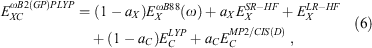
where the new mixing parameter aC is introduced. Note the initial restriction of (1−aC) for the DFT term; however, some later DHDFAs variants have lifted that requirement.[26,91–93] Similar to a conventional MP2 calculation in WFT, where a HF calculation precedes the perturbative step, a DH calculation also consists of two steps. The first step is a usual ground-state DFT SCF calculation for the first three components of Eqn 3, that is, a hybrid-DFT step that generates converged MOs and their energies (see the schematic representation in Fig. 3). These occupied and virtual MOs as well as their energies are subsequently used for the perturbative step, which in essence is an energy correction that does not change the underlying orbitals and density; for DHDFAs that do adjust their orbitals, see Refs [94–96].
|
Critics of DHDFAs may argue that similar to MP2 the formal computational cost rises; however, we refer to our previous account that lists techniques to speed up the perturbative step[6] as well as more recent developments.[97] Furthermore, even if the cost is comparable to MP2 and a user may be inclined to use that established WFT methodology instead, it has been convincingly demonstrated that DHDFAs outperform MP2 by far.[24,98] In fact, the currently most accurate and robust DFAs for ground-state properties, particularly of main-group elements, are double hybrids.[6,23,24,26,27,99]
The first global DHDFA that followed Eqn 3 is Grimme’s B2PLYP functional from 2006.[89] It is a semi-empirical DFA based on Becke-88[38] (B88) exchange and Lee-Yang-Parr[39,40] (LYP) correlation with 53 % Fock exchange and 27 % perturbative correlation. The list of currently available semi- and non-empirical DHDFAs is exhaustive and can be obtained from Refs [24, 27, and 90].
Time-Dependent Formalism for Double Hybrids
One year after the formulation of B2PLYP and before the rapid increase in the number of ground-state DHDFAs, Grimme and Neese suggested B2PLYP’s logical extension to access vertical excitation energies at the DH level.[9] The schematic idea behind this is depicted in Fig. 3. While a hybrid-type energy is perturbatively corrected through an MP2-like step in ground-state DHDFAs, TD-DHDFAs rely on a hybrid-like excitation energy that is subsequently also corrected by a second-order perturbative term to better describe the effect of electron correlation on the excitation energy. The steps in a TD-DHDFA calculation are therefore as follows (see Fig. 3): a ground-state SCF calculation is carried out with the first three components of Eqn 3 and the resulting MOs, their energies, and the hybrid component of the DHDFA are used as an input for a standard TD-DFT treatment according to Eqn 2. This results in the hybrid-component ΔEhybrid−TD−DFT of the total double-hybrid excitation energy ΔETD−DHDFA. For the perturbative part, an equivalent to MP2 for the excited state needed to be found. Grimme and Neese suggested to use Head-Gordon and co-workers’ Configuration Interaction Singles with Perturbative Doubles Correction [CIS(D)] approach, which was introduced in 1994 as an electron-correlation correction to excitation energies obtained with the CIS WFT approach.[107] The DHDFDA excitation energy can therefore be expressed as:

where  is the perturbative correction to the excitation energy and aC is the same scale factor as for the ground-state DHDFA (see Eqn 3).
Having defined the time-dependent version of DHDFAs, we conclude with a number of technical comments before we review the performance of the first-generation TD-DHDFAs that follow Grimme and Neese’s scheme. The original CIS(D) relies on underlying CIS excitation energies, excitation amplitudes and the underlying ground-state orbitals. When applying the CIS(D) correction to TD-DFT excitations, Grimme and Neese suggested to only involve the excitation vector X (Eqn 2) as an input for the perturbative correction, while Y is neglected. When the TDA is used, the resulting TDA-DFT step only involves the vector X, and thus TDA-DHDFAs are a straightforward analogy to the CIS(D) WFT problem. The CIS(D) correction is only an energy correction, which means other quantities, such as transition dipole moments and their related oscillator and rotational strengths, have hybrid quality. Finally, note that the MP2-like ground-state step is not required if one is solely interested in excitation energies, as that step does not change the MOs required for the TD-DFT component.
In 2017, the basis-set dependence of TD(A)-DHDFAs was assessed for methods with large and small CIS(D) portions—large and small aC—and was reported to be low for valence and Rydberg excitations when comparing a large quadruple- with a large triple-ζ basis set.[7] Even for full CIS(D) (aC = 1), for which the largest basis-set dependence is expected, a maximum difference of only 0.03 eV in the excitation energies for valence and Rydberg excitations was reported.[7] This indicates that using TD(A)-DHDFAs with a reliable triple-ζ basis set, such as (aug-)cc-pVTZ[108,109] or def2-TZVP(D),[110,111] seems to be sufficient in both benchmark studies and applications.
While the additional CIS(D) step comes with an overall increase in computer time, we noticed that for chromophores such as benzene and naphthalene only 2-4 % of the time needed to calculate the first excitation energy is dedicated to the CIS(D) correction in our implementation. This fraction is expected to increase for larger systems, but in our experience the CIS(D) component has not posed any major challenges yet for medium-sized molecules as long as enough memory can be provided. Similar techniques to speed up the MP2 ground-state calculation can also be used for CIS(D).
Early papers that reported full TD-DHDFA results were limited to a local code that was not accessible to the general user. TDA-DHDFAs have been accessible in older versions of the program ORCA, while full TD-DHFAs have become available in 2018 in ORCA 4.1.[112] They are therefore now available to the general user. Table 1 shows information for those TD(A)-DHDFAs that we mention in the following sections and that have been thoroughly tested in the literature.

|
2007-2016: Early Successes of Time-Dependent Double Hybrids
The success of the first TD-DHDFA following Grimme and Neese’s definition in Eqn 4 was demonstrated for B2PLYP in 2007, mostly for singlet-singlet excitations in a series of closed-shell organic molecules and a few transition-metal compounds, such as ferrocene; experimental data were predominantly used as a benchmark. Both TD-B2PLYP and TDA-B2PLYP showed smaller average errors compared to the common hybrid TD(A)-B3LYP. Including the CIS(D) correction usually led to a redshift and an error reduction of about 0.3 eV compared to the TD-DFT hybrid portion of B2PLYP, which justified the additional computational expense for the perturbative step. The 2007 paper also showed promising results for TDA-B2PLYP for singlet-triplet transitions in small (in)organic molecules, as well as doublet-doublet transitions in small radicals.
All subsequent works on DHDFAs for excited states focussed almost exclusively on full TD-DFT treatments of singlet-singlet transitions in organic systems. In 2009 and 2010, the TD-DHDFA idea was applied for the first time to the B2GPPLYP functional, which outperformed TD-B2PLYP on a popular and comprehensive test set by Thiel and co-workers[113] for small organic molecules, as well as for the aforementioned large-dye test set shown in Fig. 2. While the best 4th-rung functional for the dye set is PBE38, closely followed by BMK and CAM-B3LYP (Fig. 2), both B2PLYP and B2GPPLYP showed even better results, making them the best TD-DFT methods for this set: MD = −0.07 eV and MAD = 0.16 eV (B2PLYP), and MD = 0.03 eV and MAD = 0.14 eV (B2GPPLYP).[61] In 2013, the non-empirical methods PBE0-DH and PBE0-2 were assessed on the same set, but only in their TDA versions. A comparison with TD-B2(GP)PLYP showed that the non-empirical methods were on average up to 0.08 eV worse.[90] The fact that the phrase ‘non-empirical’ should not be misunderstood as a label for quality or reliability was later also demonstrated for DHDFAs applied to ground-state properties, where semi-empirical approaches by far outperformed non-empirical ones.[24]
In the context of TD(A)-DHDFAs, it is also worthwhile considering the pure CIS(D) WFT approach upon which the Grimme-Neese scheme is based. For the same dye test set, CIS(D) WFT only delivered an MD and MAD of 0.25 eV.[61] This demonstrates the benefit of merging DFT with WFT parts, as is done in DHDFAs. The gold standard approximate coupled-cluster approach CC2[114] was reported to have an MD of 0.04 eV and an MAD of 0.14 eV.[61] Given that it is computationally more demanding than TD-DHDFAs, this finding makes the latter a promising alternative. TD-B2PLYP and TD-B2GPPLYP also showed very promising results for extended polycyclic aromatic hydrocarbons (PAHs),[115] and we will return to PAHs in a later section to also include a discussion of our latest developments.
In the section Recommendations and Warnings for Organic Molecules, we mentioned the problem of artificial ghost states. Due to their high fraction of Fock exchange (Table 1), DHDFAs are practically free from that problem. Coming back to the specific example of the large macrocycle for which 62 states had been calculated with TD-PBE and 34 with TD-B3LYP, TD-B2GPPLYP only needed 12 genuine states.[68] While the calculation for each individual state is more costly due to the additional CIS(D) step, the overall duration for obtaining the entire ECD spectrum is shorter, as fewer states have to be calculated.
TD-DHDFAs have also been successfully used in absorption spectroscopies, in particular ECD spectroscopy. This was first done on a set of six systems with accurate experimental data, for which TD-B2PLYP outperformed the often applied TD-B3LYP approach,[67] which incidentally was originally designed for the related vibrational CD spectroscopy.[70] Compared to TD-B3LYP, TD-B2PLYP did not only solve the problem of artificial ECD bands, but it also provided improved band positions, which made the often used strategy to apply a constant shift to all ECD bands void. It therefore became a promising candidate for the computational determination of absolute configurations of molecules.
Another important finding on TD-DHDFAs in the context of ECD spectroscopy is the little-known fact that they were the only TD-DFT methods that could successfully reproduce an exciton-coupled spectrum of a merocyanine dimer aggregate.[68] Initially, only WFT methods were capable of reproducing this spectrum,[116] while lower rung functionals, including RS hybrids DFAs, failed to provide the actual bands in the spectrum associated with exciton coupling.[68] TD-B2GPPLYP, on the other hand, showed perfect agreement and again without the emergence of any artificial states.[68]
The good performance of DHDFAs for electronic excitation energies has also been confirmed in subsequent studies; however, most of them only made use of the TDA-DFT variant due to a lack of a readily available full TD-DFT code at that time.[101,104,117–124]
2017: Modifying the Electron-Correlation Term
Spin-Component- and Spin-Opposite-Scaling Techniques
Whenever discussing DHDFAs, it is worthwhile to draw analogies to the closely related MP2 theory for ground states. While MP2 was theoretically formulated in 1934[125] and has been a crucial component of conventional quantum-chemical software for decades, it was only in 2003 that Grimme suggested to break the MP2 correlation energy down into two separate components with the first being the sum of all possible pair correlation energies of electron pairs of same spin (SS) and the second the sum of all pair-correlation energies of opposite spin (OS).[126] Each component is then separately scaled according to:

where the values for the two scaling parameters are  and
and  . The rationale behind this spin-component-scaling (SCS) idea is that HF Theory already includes SS correlation—also known as Fermi correlation—through the incorporation of exchange terms. Therefore, conventional MP2 overestimates Fermi correlation in a molecule and its MP2 contribution should be scaled down. The values of the two scale parameters were determined semi-empirically, but subsequent theoretical derivations of this and very similar theories derived very similar values.[127,128] In 2004, Head-Gordon and co-workers suggested to ignore the SS term, as this would allow the implementation of a very efficient algorithm[129] that brings the formal scaling behaviour of MP2 down from
  to
to  , with N being the system size or number of atomic orbitals; this approach is abbreviated as spin-opposite-scaling (SOS).[130]
Both the SCS and SOS approaches have been adopted by other WFT methods for both ground and excited states; Ref. [131] provides a detailed overview of them. For our context, we only mention that the CIS(D) approach was first combined with SCS in 2004[132] followed by further modifications and extension to SOS in 2007.[133] In the following discussion, we always refer to the 2007 implementation. When applied to systems 1-11 in the aforementioned dye test set (Fig. 2), reductions of 0.07-0.08 eV compared to CIS(D) were reported with SCS- and SOS-CIS(D) performing very similarly. That being said, SCS/SOS-CIS(D) were still topped by TD-B2PLYP and TD-B2GPPLYP. SCS-CIS(D) also showed very promising results for the exciton-coupled ECD spectrum for the aforementioned merocyanine dimer aggregate in the section 2007–2016: Early Successes of Time Dependent Double Hybrids.[116]
The SCS/SOS-MP2 ideas have also been applied since 2008 in the context of DHDFAs with developments by Chai and Head-Gordon, Kozuch and Martin, and Goerigk and Grimme being the first of their type. Amongst the DHDFAs with SCS, ωB97X-2,[134] DSD-BLYP, and DSD-PBEP86 belong to the best for main-group ground-state problems,[24] while the best SOS-based DHDFAs are DOD-SCAN[26] and revDOD-PBEP86.[26] The SOS-based method PWPB95[135] showed promising results for transition-metal problems.[135,136]
Time-Dependent Double Hybrids with Component-Scaled Correlation Term
Based on the success of ground-state SCS/SOS-DHDFAs and the improved results for SCS/SOS-CIS(D) for excited states, the logical step forward was to also apply the same ideas to TD-DHDFAs. Schwabe and Goerigk did so in 2017 and presented different variants of six functionals, namely B2PLYP, B2GPPLYP, PBE0-DH, PBE0-2, DSD-BLYP and DSD-PBEP86 (see Table 1).[7] For each functional, up to four scaled variants were tested that differed in their degree of empiricism. Such complexity was necessary because opposed to ground-state SCS-MP2 in Eqn 5, two parameters each are needed for the SS and OS components of SCS-CIS(D).[133] Schwabe and Goerigk tested an empirical least-squares fit of all four parameters (SCS variants), a combination of non-empirical parameters and empirical fits (SCS variants), non-empirical SCS-variants, as well as an empirical fit of the two OS-parameters (SOS variants). The empirical fits were carried out against a new training set of small, organic chromophores for which highly accurate ab-initio WFT reference data were presented. Note that such a fit is to be favoured over fitting against experimental data, as any vibrational or solvent effects should not be included during such a fit. Ultimately, the developed methods are designed to get the electronic structure right. Solvent effects should be addressed by an appropriate solvent model, for instance. The fit set contained a mixture of local-valence and Rydberg excitations. Fits were separately carried out for the TD-DFT and TDA-DFT approaches. In some cases, an SCS approach automatically resulted in the SOS version during the fit, for instance in the case of TD-SCS-B2PLYP and TD-SCS-PBE0-DH. Note that the two DSD methods already contained SCS parameters optimised for ground-states. The 2017 study tested those original versions as well as the refits.
Cross-validation studies were carried out for vertical local-valence and Rydberg excitations with the aforementioned popular set by Thiel and co-workers[113] as well as on an updated version of a test set initially assembled by Gordon and co-workers;[62] see Ref. [7] for updated geometries and highly accurate WFT reference values. Additional tests were also conducted on a series of 0-0 excitations in organic chromophores initially presented as an individual test set in Ref. [137]. Overall, both the SCS and SOS variants constituted an improvement over the global DHDFAs. The following methods were particularly useful, sometimes showing results within the chemical accuracy threshold: the newly fitted SOS and SCS versions of TD-B2GPPLYP, the newly fitted SOS versions of both TD-B2PLYP and TD-PBE0-DH, and the original ground-state SCS-version of DSD-PBEP86, which makes the latter particularly promising for simultaneously accurate treatments of ground and excited state properties.
While SCS and SOS variants of TD(A)-DHDFAs have shown very promising results, they have not yet been made readily available to be used in actual applications, but we hope to change this in a future release of ORCA. Moreover, our group’s developments in this space have momentarily shifted away from those variants, as they suffer from the same problem as the unscaled TD(A)-DHDFAs, namely the description of CT excitations. The following section will therefore deal with those and address how we were able to successfully address this problem.
2019: The First Time-Dependent Double Hybrids with Range Separation
Charge-Transfer Excitations
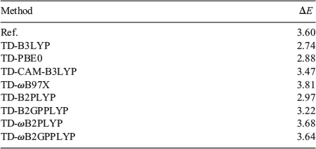
So far, we have discussed the success of TD-DHDFAs predominantly for local valence excitations; however, already in 2010 it became evident that the methods suffer from the same inherent problem as any other conventional TD-DFT methods, namely the well-known[138–140] inability to describe CT excitations. This can be exemplified for molecule 12—2,4-dichloro-6-[p-(N,N- diethylamino)biphenylyl]-1,3,5-triazine (DBQ)—which was part of the same organic-molecule test set shown in Fig. 2, but excluded from the statistics shown in the same figure. A good reference excitation energy with an expected absolute error below 0.1 eV is 3.60 eV (Table 2). The inability of conventional TD-DFT methods to describe CT excitations is shown for TD-B3LYP and TD-PBE0, which underestimate the excitation energy by 0.86 and 0.72 eV, respectively. These are larger errors than for local valence excitations. The RS technique introduced to the hybrid-DFT level rectifies the problem of underestimation somewhat, with TD-CAMB3LYP underestimating the excitation energy by only 0.13 eV. However, the RS technique at the hybrid level does not automatically solve the CT problem, as can be seen for TD-ωB97X, which exhibits a blueshift of 0.21 eV. The DHDFAs B2PLYP and B2GPPLYP show the typical underestimation of excitation energies for CT states by 0.63 and 0.38 eV, respectively. This shows the limitation of the TD-DHDFAs published from 2007–2017, which limits their applicability to real-life problems, where the boundaries between local and LR transitions may not always be well defined. We therefore disagree with the very recently made statement that the CIS(D) correction would enable a better description of CT transitions for global DHDFAs such as TDA-PBE-QIDH.[141] Such a statement is surprising because TDA-PBE-QIDH showed a systematic underestimation in the through-space CT examples discussed in that very same study.[141] We argue that RS should be applied to TD(A)-DHDFAs instead, something that seems to have been overlooked in Ref. [141] but which we will demonstrate in the following section.
|
ωB2PLYP and ωB2GPPLYP: Definition
To address the systematic underestimation of CT states with TD-DHDFAs, we introduced the RS technique to TD-B2PLYP and TD-B2GPPLYP. While the RS scheme has been applied previously to DHDFAs in the context of ground states,[56,99,134,142–145] our TD-ωB2PLYP and TD-ωB2GPPLYP approaches are the first double hybrids optimised for excited states that follow Grimme and Neese’s TD-DHDFA scheme.[8] Both methodologies follow the typical RS ansatz in which some SR-DFT exchange (ωB88[50]) is mixed with Fock exchange, while the LR region is described to 100 % with exact exchange:[8]
where the values of aX and aC are the same as for the global DHDFAs B2PLYP and B2GPPLYP. While a reoptimisation of all parameters would have been a viable option, we decided to keep our approaches as simple as possible and only determined the value of the RS parameter ω. In that way, we were able to directly investigate the influence of RS on the TD-DHDFA scheme. Our main hypothesis was to induce a redshift through the CIS(D) correction, which corrects for the blueshift induced by the RS scheme. The least-squares fit of ω was based on a slightly modified version of the training set used in 2017 for the SCS and SOS versions of global TD-DHDFAs described in the section Time-Dependent Double Hybrids with Component-Scaled Correlation Term, with the main difference being a more equal weighting of both valence and Rydberg excitations. The resulting values for the RS parameter are ω = 0.30 for TD-ωB2PLYP and ω = 0.27 for TD-ωB2GPPLYP, which are comparable to other RS DFAs.[50,99,134,145,146]
ωB2PLYP and ωB2GPPLYP: Singlet-Singlet Excitations
The main requirement during the development of both TD-ωB2PLYP and TD-ωB2GPPLYP was that the very good description of valence excitations with the underlying global parent DHDFAs was maintained, while LR excitations—Rydberg and CT—were improved. We conclude the discussion of our RS TD-DHDFAs with a brief summary of their performance showing that this goal has been achieved.
CT excitations were not included in the training set, so they provide the best cross-validation case. Using our example from Table 2, we see that indeed both approaches improve dramatically over TD-B2PLYP and TD-B2GPPLYP and provide nearly perfect excitation energies for the DBQ molecule with overestimations of only 0.08 (TD-ωB2PLYP) and 0.04 eV (TD-ωB2GPPLYP). An analysis of 17 CT excitations in nine molecules—mostly based on newly generated high-level reference data[8]—confirmed that the two RS DHDFAs improve significantly over their global parent DHDFAs (Fig. 4). Like for DBQ, the underestimation problem is fixed and at the same time the excitation energies improve, as shown for the MADs: MAD = 0.94 eV (TD-B2PLYP) versus MAD = 0.22 eV (TD-ωB2PLYP) and MAD = 0.54 eV (TD-B2GPPLYP) versus MAD = 0.33 eV (TD-ωB2GPPLYP). When comparing the new RS TD-DHDFAs with their closest competitors, namely RS hybrids, only ωB97X[146] (MAD = 0.23 eV) comes close to TD-ωB2PLYP; however, the latter is the only one of the tested approaches with an error range below 1 eV and, therefore, overall more robust.

|
Both RS TD-DHDFAs showed superior performance for all tested local-valence and Rydberg excitation test sets, with both methods showing higher robustness than global DHDFAs, global hybrids, and RS hybrids. TD-ωB2PLYP turned out to be more robust than TD-ωB2GPPLYP and a significant improvement over the original TD-B2PLYP, which had already counted as one of the best TD-DFT methods for valence excitations prior to this study (see earlier sections). TD-ωB2PLYP also met our requirement of providing valence excitation energies of at least the same quality as global DHFAs, while providing better LR excitations. We can see this, for instance, for the aforementioned updated Gordon test set for which the MADs for valence excitations stay the same when going from B2PLYP to its RS version (MAD = 0.23 eV) but dramatically improve for Rydberg excitations (MAD = 0.49 eV ve MAD = 0.16 eV).[8]
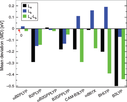
For both RS TD-DHDFAs we also reported excellent performance for PAHs. In 2003, Grimme and Parac revealed severe deficiencies of conventional TD-DFT methods when they struggled to accurately predict excitation energies and energetic order of the first two singlet excited states in linear and non-linear PAHs, the La and Lb states.[147,148] Their analysis revealed that the La state is more ionic and the Lb state more covalent in character and that conventional DFAs failed to describe both types of states equally well. Initially, RS hybrids seemed to be a solution to the problem, but closer analysis revealed that the better description of La states with RS came at the cost of a significant blueshift for the second state.[74] In 2011, Goerigk and Grimme indicated that global TD-DHDFAs partially rectified this problem,[115] but only our RS TD-DHDFAs were able to provide a truly robust description, as shown in Fig. 5 for linear PAHs, which shows statistics averaged over the linear series from naphthalene to hexacene. Not only are MDs zero or nearly zero for both states and both RS TD-DHDFAs, but also the energy splitting between both states is the most accurate. The figure also shows the aforementioned problems of RS and global hybrids with these states. The reference values for the statistics shown in Fig. 5 are based on the CC2 level of theory, which in itself has an MD of about 0.3 eV for Lb states when compared with CR-EOM-CCSD(T) data.[149,150] Regardless of the type of reference, RS TD-DHDFAs still show the best-reported results to date and are a promising step in the right direction. Findings for non-linear PAHs were equally promising.[8]
|
Summary, Potential Problems, and Next Steps
TD-DFT has become the method of choice for treating electronic excited states, but similar to ground-state DFT the field can be confusing. Some problems of conventional TD-DFT when dealing with vertical, adiabatic, or 0-0 excitations include the emergence of artificial ghost states, an inability to describe LR excitations, and a lack of robustness that may prevent the description of different types of excited states with the same accuracy. TD-DHDFAs with RS provide a promising solution to those problems and our recently developed methods ωB2PLYP and ωB2GPPLYP—particularly the first of the two—are currently some of the most accurate TD-DFT approaches for applications to singlet-singlet excitations in organic molecules. If LR excitations are not a concern, global TD-DHDFAs—B2GPPLYP or various methods with spin-component or spin-opposite scaling—may also be used. If DHDFAs cannot be applied for computational reasons, RS hybrids can be used, or global hybrids with an amount of about 40 % Fock exchange if LR excitations are not relevant. LDA, GGA or meta-GGA functionals should not be used in any TD-DFT calculations due to large redshifts and a large number of ghost states. We also recommend to run calculations with at least two different methods, which may help to distinguish between artificial and relevant results and therefore improve the reliability of any predictions.
Our new TD-DHDFAs with RS have been available for free since the release of ORCA 4.2. A full TD-DFT treatment with global DHDFAs has been available since ORCA 4.1. Older ORCA versions only allow the application of TDA-DFT with global DHDFAs, something that has been sometimes overlooked in the literature. We hope to make the previously published SCS and SOS versions available soon.
Not all, but many of the benchmarks discussed herein have CC3[151] or even higher quality for small chromophores, but slightly lower quality for bigger systems (CC2 or theoretically back-corrected experimental data). While every benchmark study rises and falls with the accuracy of its reference values, the studies we reviewed all agree with the Jacob’s Ladder picture, namely that TD(A)-DHDFAs are more robust and reliable than lower-rung methods. By reviewing most TD(A)-DHDFA benchmark studies in one article, we were able to provide additional credibility to those reported findings. We hope that with improving computational resources, better reference data can be generated in the future, which will further confirm the trends reported herein.
So far, we have only discussed results for singlet-singlet excitations in organic molecules, but we will report about our methods for singlet-triplet excitations shortly.[106] In our 2019 study, we also had a brief glimpse at the treatment of transition-metal compounds with the example of titanium dioxide monomers, dimers, and trimers.[8] While TD-DHDFAs with RS were better than global ones, their accuracy was the same as for RS hybrids and overall not as good as global hybrids. There is therefore room for further investigations and developments in this space.
Double hybrids are of course not a panacea for every problem. Other known problems of TD-DFT, such as the inability to describe conical intersections,[152] are unlikely to be solved, for instance. Due to the perturbative correction, higher-lying excited states, low-gap systems, and other (nearly) degenerate states are unlikely to be treated. Geometry optimisations of excited states are currently not possible; however, based on knowledge gained from ground-state treatments,[153] hybrid functionals should already provide accurate enough geometries in standard cases. Nevertheless, these examples show that the story of time-dependent double hybrids has not come to an end and more exciting developments are yet to come.
Conflicts of Interest
The authors declare no conflicts of Interest.
Acknowledgements
L. G. would like to thank Prof. Stefan Grimme for introducing him to double-hybrid DFT as well as past collaborators on time-dependent double-hybrids, in particular Dr Tobias Schwabe. L. G. is humbled and immensely grateful to the Australian Academy of Science for being the recipient of a 2019 Le Fèvre Medal. Generous resource allocations from the former Melbourne Bioinformatics (Project RA0005) and the National Computational Infrastructure (NCI) National Facility within the National Computational Merit Allocation Scheme (Project fk5) over the past years are highly acknowledged as well as high-performance computing support by The University of Melbourne. M. C.-P acknowledges a ‘Melbourne Research Scholarship’ by The University of Melbourne.
References
[1] P. Hohenberg, W. Kohn, Phys. Rev. 1964, 136, B864.| Crossref | GoogleScholarGoogle Scholar |
[2] W. Kohn, L. J. Sham, Phys. Rev. 1965, 140, A1133.
| Crossref | GoogleScholarGoogle Scholar |
[3] E. Runge, E. K. U. Gross, Phys. Rev. Lett. 1984, 52, 997.
| Crossref | GoogleScholarGoogle Scholar |
[4] E. K. U. Gross, W. Kohn, Adv. Quantum Chem. 1990, 21, 255.
| Crossref | GoogleScholarGoogle Scholar |
[5] R. Bauernschmitt, R. Ahlrichs, Chem. Phys. Lett. 1996, 256, 454.
| Crossref | GoogleScholarGoogle Scholar |
[6] L. Goerigk, N. Mehta, Aust. J. Chem. 2019, 72, 563.
| Crossref | GoogleScholarGoogle Scholar |
[7] T. Schwabe, L. Goerigk, J. Chem. Theory Comput. 2017, 13, 4307.
| Crossref | GoogleScholarGoogle Scholar | 28763220PubMed |
[8] M. Casanova-Páez, M. B. Dardis, L. Goerigk, J. Chem. Theory Comput. 2019, 15, 4735.
| Crossref | GoogleScholarGoogle Scholar | 31298850PubMed |
[9] S. Grimme, F. Neese, J. Chem. Phys. 2007, 127, 154116.
| Crossref | GoogleScholarGoogle Scholar | 17949141PubMed |
[10] M. E. Casida, in Recent Advances in Density Functional Methods (Ed. D. P. Chong) 1995, pp. 155–192 (World Scientific: Singapore).
[11] M. E. Casida, J. Mol. Struct. THEOCHEM 2009, 914, 3.
| Crossref | GoogleScholarGoogle Scholar |
[12] M. Marques, N. Maitra, F. Nogueira, E. Gross, A. Rubio, Fundamentals of Time-Dependent Density Functional Theory; Lecture Notes in Physics 2012 (Springer: Berlin).
[13] C. Ullrich, Time-Dependent Density Functional Theory: Concepts and Applications 2017 (Oxford University Press: Oxford).
[14] Time-Dependent Density Functional Theory (Eds M. A. L. Marques, C. A. Ullrich, F. Nogueira, A. Rubio, K. Burke, E. K. U. Gross) 2006 (Springer-Verlag: Berlin).
[15] M. A. L. Marques, E. K. U. Gross, Annu. Rev. Phys. Chem. 2004, 55, 427.
| Crossref | GoogleScholarGoogle Scholar |
[16] F. Jensen, Introduction to Computational Chemistry, 3rd edn 2017. (John Wiley and Sons: Hoboken, NJ).
[17] W. Koch, C. M. Holthausen, A Chemist’s Guide to Density Functional Theory, 2nd edn 2001 (Wiley-VCH: Weinheim).
[18] E. Sim, S. Song, K. Burke, J. Phys. Chem. Lett. 2018, 9, 6385.
| Crossref | GoogleScholarGoogle Scholar | 30335392PubMed |
[19] J. L. Bao, L. Gagliardi, D. G. Truhlar, J. Phys. Chem. Lett. 2018, 9, 2353.
| Crossref | GoogleScholarGoogle Scholar | 29624392PubMed |
[20] D. Hait, M. Head-Gordon, J. Phys. Chem. Lett. 2018, 9, 6280.
| Crossref | GoogleScholarGoogle Scholar | 30339010PubMed |
[21] S. Vuckovic, S. Song, J. Kozlowski, E. Sim, K. Burke, J. Chem. Theory Comput. 2019, 15, 6636.
| Crossref | GoogleScholarGoogle Scholar | 31682433PubMed |
[22] D. R. Lonsdale, L. Goerigk, Phys. Chem. Chem. Phys. 2020,
| Crossref | GoogleScholarGoogle Scholar | 32458849PubMed |
[23] L. Goerigk, A. Hansen, C. Bauer, S. Ehrlich, A. Najibi, S. Grimme, Phys. Chem. Chem. Phys. 2017, 19, 32184.
| Crossref | GoogleScholarGoogle Scholar | 29110012PubMed |
[24] N. Mehta, M. Casanova-Páez, L. Goerigk, Phys. Chem. Chem. Phys. 2018, 20, 23175.
| Crossref | GoogleScholarGoogle Scholar | 30062343PubMed |
[25] A. Najibi, L. Goerigk, J. Chem. Theory Comput. 2018, 14, 5725.
| Crossref | GoogleScholarGoogle Scholar | 30299953PubMed |
[26] G. Santra, N. Sylvetsky, J. M. L. Martin, J. Phys. Chem. A 2019, 123, 5129.
| Crossref | GoogleScholarGoogle Scholar | 31136709PubMed |
[27] J. M. L. Martin, G. Santra, Isr. J. Chem. 2019,
| Crossref | GoogleScholarGoogle Scholar |
[28] L. Goerigk, S. Grimme, J. Chem. Theory Comput. 2010, 6, 107.
| Crossref | GoogleScholarGoogle Scholar | 26614324PubMed |
[29] J. P. Perdew, K. Schmidt, AIP Conf. Proc. 2001, 577, 1.
| Crossref | GoogleScholarGoogle Scholar |
[30] R. Send, M. Kühn, F. Furche, J. Chem. Theory Comput. 2011, 7, 2376.
| Crossref | GoogleScholarGoogle Scholar | 26606613PubMed |
[31] P.-F. Loos, N. Galland, D. Jacquemin, J. Phys. Chem. Lett. 2018, 9, 4646.
| Crossref | GoogleScholarGoogle Scholar | 30063359PubMed |
[32] S. Grimme, in Reviews in Computational Chemistry (Eds K. B. Lipkowitz, D. B. Boyd) 2004, Vol. 20, pp. 153–218 (Wiley-VCH: New York, NY).
[33] L. Goerigk, J. Moellmann, S. Grimme, Phys. Chem. Chem. Phys. 2009, 11, 4611.
| Crossref | GoogleScholarGoogle Scholar | 19475182PubMed |
[34] P.-F. Loos, P. M. W. Gill, Wiley Interdiscip. Rev. Comput. Mol. Sci. 2016, 6, 410.
| Crossref | GoogleScholarGoogle Scholar |
[35] J. C. Slater, Rev. Phys. 1951, 81, 385.
| Crossref | GoogleScholarGoogle Scholar |
[36] S. J. Vosko, L. Wilk, M. Nusair, Can. J. Phys. 1980, 58, 1200.
| Crossref | GoogleScholarGoogle Scholar |
[37] J. P. Perdew, Y. Wang, Phys. Rev. B Condens. Matter 1992, 45, 13244.
| Crossref | GoogleScholarGoogle Scholar | 10001404PubMed |
[38] A. D. Becke, Phys. Rev. A 1988, 38, 3098.
| Crossref | GoogleScholarGoogle Scholar |
[39] C. Lee, W. Yang, R. G. Parr, Phys. Rev. B Condens. Matter 1988, 37, 785.
| Crossref | GoogleScholarGoogle Scholar | 9944570PubMed |
[40] B. Miehlich, A. Savin, H. Stoll, H. Preuss, Chem. Phys. Lett. 1989, 157, 200.
| Crossref | GoogleScholarGoogle Scholar |
[41] J. P. Perdew, K. Burke, M. Ernzerhof, Phys. Rev. Lett. 1996, 77, 3865.
| Crossref | GoogleScholarGoogle Scholar | 10062328PubMed |
[42] J. P. Perdew, Phys. Rev. B Condens. Matter 1986, 33, 8822.
| Crossref | GoogleScholarGoogle Scholar | 9938299PubMed |
[43] J. P. Perdew, Phys. Rev. B Condens. Matter 1986, 34, 7406.
| Crossref | GoogleScholarGoogle Scholar | 9949100PubMed |
[44] J. P. Perdew, S. Kurth, A. Zupan, P. Blaha, Phys. Rev. Lett. 1999, 82, 2544.
| Crossref | GoogleScholarGoogle Scholar |
[45] J. Tao, J. P. Perdew, V. N. Staroverov, G. E. Scuseria, Phys. Rev. Lett. 2003, 91, 146401.
| Crossref | GoogleScholarGoogle Scholar | 14611541PubMed |
[46] A. D. Becke, J. Chem. Phys. 1993, 98, 1372.
| Crossref | GoogleScholarGoogle Scholar |
[47] T. M. Maier, A. V. Arbuznikov, M. Kaupp, Wiley Interdiscip. Rev. Comput. Mol. Sci. 2019, 9, e1378.
| Crossref | GoogleScholarGoogle Scholar |
[48] T. Leininger, H. Stoll, H.-J. Werner, A. Savin, Chem. Phys. Lett. 1997, 275, 151.
| Crossref | GoogleScholarGoogle Scholar |
[49] H. Iikura, T. Tsuneda, T. Yanai, K. Hirao, J. Chem. Phys. 2001, 115, 3540.
| Crossref | GoogleScholarGoogle Scholar |
[50] T. Yanai, D. P. Tew, N. C. Handy, Chem. Phys. Lett. 2004, 393, 51.
| Crossref | GoogleScholarGoogle Scholar |
[51] R. Baer, D. Neuhauser, Phys. Rev. Lett. 2005, 94, 043002.
| Crossref | GoogleScholarGoogle Scholar | 15783554PubMed |
[52] I. C. Gerber, J. G. Ángyán, M. Marsman, G. Kresse, J. Chem. Phys. 2007, 127, 054101.
| Crossref | GoogleScholarGoogle Scholar | 17688328PubMed |
[53] E. Livshits, R. Baer, Phys. Chem. Chem. Phys. 2007, 9, 2932.
| Crossref | GoogleScholarGoogle Scholar | 17551616PubMed |
[54] R. Baer, E. Livshits, U. Salzner, Annu. Rev. Phys. Chem. 2010, 61, 85.
| Crossref | GoogleScholarGoogle Scholar | 20055678PubMed |
[55] O. A. Vydrov, J. Heyd, A. V. Krukau, G. E. Scuseria, J. Chem. Phys. 2006, 125, 074106.
| Crossref | GoogleScholarGoogle Scholar | 16942321PubMed |
[56] E. Bremond, A. J. Perez-Jimenez, J. C. Sancho-Garcia, C. Adamo, J. Chem. Phys. 2019, 150, 201102.
| Crossref | GoogleScholarGoogle Scholar | 31153220PubMed |
[57] T. M. Henderson, A. F. Izmaylov, G. E. Scuseria, A. Savin, J. Chem. Phys. 2007, 127, 221103.
| Crossref | GoogleScholarGoogle Scholar | 18081380PubMed |
[58] A. D. McLachlan, M. A. Ball, Rev. Mod. Phys. 1964, 36, 844.
| Crossref | GoogleScholarGoogle Scholar |
[59] S. Hirata, M. Head-Gordon, Chem. Phys. Lett. 1999, 314, 291.
| Crossref | GoogleScholarGoogle Scholar |
[60] M. R. Silva-Junior, M. Schreiber, S. P. A. Sauer, W. Thiel, J. Chem. Phys. 2008, 129, 104103.
| Crossref | GoogleScholarGoogle Scholar | 19044904PubMed |
[61] L. Goerigk, S. Grimme, J. Chem. Phys. 2010, 132, 184103.
| Crossref | GoogleScholarGoogle Scholar |
[62] S. S. Leang, F. Zahariev, M. S. Gordon, J. Chem. Phys. 2012, 136, 104101.
| Crossref | GoogleScholarGoogle Scholar | 22423822PubMed |
[63] D. Jacquemin, V. Wathelet, E. A. Perpète, C. Adamo, J. Chem. Theory Comput. 2009, 5, 2420.
| Crossref | GoogleScholarGoogle Scholar | 26616623PubMed |
[64] C. Suellen, R. G. Freitas, P.-F. Loos, D. Jacquemin, J. Chem. Theory Comput. 2019, 15, 4581.
| Crossref | GoogleScholarGoogle Scholar | 31265781PubMed |
[65] C. Adamo, D. Jacquemin, Chem. Soc. Rev. 2013, 42, 845.
| Crossref | GoogleScholarGoogle Scholar | 23117144PubMed |
[66] A. D. Laurent, D. Jacquemin, Int. J. Quantum Chem. 2013, 113, 2019.
| Crossref | GoogleScholarGoogle Scholar |
[67] L. Goerigk, S. Grimme, J. Phys. Chem. A 2009, 113, 767.
| Crossref | GoogleScholarGoogle Scholar | 19102628PubMed |
[68] L. Goerigk, H. Kruse, S. Grimme, in Comprehensive Chiroptical Spectroscopy: Instrumentation, Methodologies, and Theoretical Simulations (Eds N. Berova, P. L. Polavarapu, K. Nakanishi, R. W. Woody) 2012, Vol. 1, Ch. 22, pp. 643–673 (Wiley-Blackwell: Chichester).
[69] A. D. Becke, J. Chem. Phys. 1993, 98, 5648.
| Crossref | GoogleScholarGoogle Scholar |
[70] P. J. Stephens, F. J. Devlin, C. F. Chabalowski, M. J. Frisch, J. Phys. Chem. 1994, 98, 11623.
| Crossref | GoogleScholarGoogle Scholar |
[71] C. Adamo, V. Barone, J. Chem. Phys. 1999, 110, 6158.
| Crossref | GoogleScholarGoogle Scholar |
[72] M. Ernzerhof, G. E. Scuseria, J. Chem. Phys. 1999, 110, 5029.
| Crossref | GoogleScholarGoogle Scholar |
[73] J. L. Alonso-Gómez, P. Rivera-Fuentes, N. Harada, N. Berova, F. Diederich, Angew. Chem. Int. Ed. 2009, 48, 5545.
| Crossref | GoogleScholarGoogle Scholar |
[74] R. M. Richard, J. M. Herbert, J. Chem.Theory Comput. 2011, 7, 1296.
| Crossref | GoogleScholarGoogle Scholar | 26610124PubMed |
[75] J. E. Bates, F. Furche, J. Chem. Phys. 2012, 137, 164105.
| Crossref | GoogleScholarGoogle Scholar | 23126693PubMed |
[76] R. M. Irelan, T. M. Henderson, G. E. Scuseria, J. Chem. Phys. 2011, 135, 094105.
| Crossref | GoogleScholarGoogle Scholar | 21913751PubMed |
[77] H. Eshuis, F. Furche, J. Phys. Chem. Lett. 2011, 2, 983.
| Crossref | GoogleScholarGoogle Scholar |
[78] A. J. Garza, I. W. Bulik, A. G. S. Alencar, J. Sun, J. P. Perdew, G. E. Scuseria, Mol. Phys. 2016, 114, 997.
| Crossref | GoogleScholarGoogle Scholar |
[79] S. Grimme, M. Steinmetz, Phys. Chem. Chem. Phys. 2016, 18, 20926.
| Crossref | GoogleScholarGoogle Scholar | 26695184PubMed |
[80] P. D. Mezei, G. I. Csonka, A. Ruzsinszky, M. Kállay, J. Chem. Theory Comput. 2015, 11, 4615.
| Crossref | GoogleScholarGoogle Scholar | 26574252PubMed |
[81] P. D. Mezei, G. I. Csonka, A. Ruzsinszky, M. Kállay, J. Chem. Theory Comput. 2017, 13, 796.
| Crossref | GoogleScholarGoogle Scholar | 28052197PubMed |
[82] B. Chan, L. Goerigk, L. Radom, J. Comput. Chem. 2016, 37, 183.
| Crossref | GoogleScholarGoogle Scholar | 26135403PubMed |
[83] R. J. Bartlett, I. Grabowski, S. Hirata, S. Ivanov, J. Chem. Phys. 2005, 122, 034104.
| Crossref | GoogleScholarGoogle Scholar |
[84] I. V. Schweigert, V. F. Lotrich, R. J. Bartlett, J. Chem. Phys. 2006, 125, 104108.
| Crossref | GoogleScholarGoogle Scholar | 16999516PubMed |
[85] A. Görling, M. Levy, Phys. Rev. B Condens. Matter 1993, 47, 13105.
| Crossref | GoogleScholarGoogle Scholar | 10005612PubMed |
[86] A. Görling, M. Levy, Phys. Rev. A 1994, 50, 196.
| Crossref | GoogleScholarGoogle Scholar | 9910882PubMed |
[87] Y. Zhao, B. J. Lynch, D. G. Truhlar, J. Phys. Chem. A 2004, 108, 4786.
| Crossref | GoogleScholarGoogle Scholar |
[88] Y. Zhao, B. J. Lynch, D. G. Truhlar, Phys. Chem. Chem. Phys. 2005, 7, 43.
| Crossref | GoogleScholarGoogle Scholar |
[89] S. Grimme, J. Chem. Phys. 2006, 124, 034108.
| Crossref | GoogleScholarGoogle Scholar | 16438568PubMed |
[90] L. Goerigk, S. Grimme, Wiley Interdiscip. Rev. Comput. Mol. Sci. 2014, 4, 576.
| Crossref | GoogleScholarGoogle Scholar |
[91] S. Kozuch, D. Gruzman, J. M. L. Martin, J. Phys. Chem. C 2010, 114, 20801.
| Crossref | GoogleScholarGoogle Scholar |
[92] S. Kozuch, J. M. L. Martin, Phys. Chem. Chem. Phys. 2011, 13, 20104.
| Crossref | GoogleScholarGoogle Scholar | 21993810PubMed |
[93] S. Kozuch, J. M. L. Martin, J. Comput. Chem. 2013, 34, 2327.
| 23983204PubMed |
[94] R. Peverati, M. Head-Gordon, J. Chem. Phys. 2013, 139, 024110.
| Crossref | GoogleScholarGoogle Scholar | 23862932PubMed |
[95] J. C. Sancho-Garcia, A. J. Perez-Jimenez, M. Savarese, E. Bremond, C. Adamo, J. Phys. Chem. A 2016, 120, 1756.
| Crossref | GoogleScholarGoogle Scholar | 26901447PubMed |
[96] A. Najibi, L. Goerigk, J. Phys. Chem. A 2018, 122, 5610.
| Crossref | GoogleScholarGoogle Scholar | 29847940PubMed |
[97] G. M. J. Barca, S. C. McKenzie, N. J. Bloomfield, A. T. B. Gilbert, P. M. W. Gill, J. Chem. Theory Comput. 2020, 16, 1568.
| Crossref | GoogleScholarGoogle Scholar |
[98] L. Goerigk, S. Grimme, Phys. Chem. Chem. Phys. 2011, 13, 6670.
| Crossref | GoogleScholarGoogle Scholar | 21384027PubMed |
[99] N. Mardirossian, M. Head-Gordon, J. Chem. Phys. 2018, 148, 241736.
| Crossref | GoogleScholarGoogle Scholar | 29960332PubMed |
[100] A. Karton, A. Tarnopolsky, J.-F. Lamère, G. C. Schatz, J. M. L. Martin, J. Phys. Chem. A 2008, 112, 12868.
| Crossref | GoogleScholarGoogle Scholar | 18714947PubMed |
[101] F. D. Meo, P. Troiullasa, C. Adamo, J. C. Sancho-García, J. Chem. Phys. 2013, 139, 164104.
| Crossref | GoogleScholarGoogle Scholar |
[102] E. Brémond, C. Adamo, J. Chem. Phys. 2011, 135, 024106.
| Crossref | GoogleScholarGoogle Scholar | 21766924PubMed |
[103] J.-D. Chai, S.-P. Mao, Chem. Phys. Lett. 2012, 538, 121.
| Crossref | GoogleScholarGoogle Scholar |
[104] E. Brémond, J. C. Sancho-García, A. J. Pérez-Jiménez, C. Adamo, J. Chem. Phys. 2014, 141, 031101.
| Crossref | GoogleScholarGoogle Scholar | 25053294PubMed |
[105] L. Hernández-Martínez, E. Brémond, A. J. Pérez-Jiménez, E. San-Fabián, C. Adamo, J. C. Sancho-García, Int. J. Quantum Chem. 2020, 120, e26193.
| Crossref | GoogleScholarGoogle Scholar |
[106] M. Casanova-Páez, L. Goerigk, manuscript under review. Preprint available on Arxiv: arXiv:2006.07821.
[107] M. Head-Gordon, R. J. Rico, M. Oumi, T. J. Lee, Chem. Phys. Lett. 1994, 219, 21.
| Crossref | GoogleScholarGoogle Scholar |
[108] T. H. Dunning, J. Chem. Phys. 1989, 90, 1007.
| Crossref | GoogleScholarGoogle Scholar |
[109] R. A. Kendall, T. H. Dunning, R. J. Harrison, J. Chem. Phys. 1992, 96, 6796.
| Crossref | GoogleScholarGoogle Scholar |
[110] F. Weigend, R. Ahlrichs, Phys. Chem. Chem. Phys. 2005, 7, 3297.
| Crossref | GoogleScholarGoogle Scholar | 16240044PubMed |
[111] D. Rappoport, F. Furche, J. Chem. Phys. 2010, 133, 134105.
| Crossref | GoogleScholarGoogle Scholar | 20942521PubMed |
[112] F. Neese, Wiley Interdiscip. Rev. Comput. Mol. Sci. 2012, 2, 73.
| Crossref | GoogleScholarGoogle Scholar |
[113] M. Schreiber, M. R. Silva-Junior, S. P. A. Sauer, W. Thiel, J. Chem. Phys. 2008, 128, 134110.
| Crossref | GoogleScholarGoogle Scholar | 18397056PubMed |
[114] O. Christiansen, H. Koch, P. Jørgensen, Chem. Phys. Lett. 1995, 243, 409.
| Crossref | GoogleScholarGoogle Scholar |
[115] L. Goerigk, S. Grimme, J. Chem. Theory Comput. 2011, 7, 3272.
| Crossref | GoogleScholarGoogle Scholar | 26598161PubMed |
[116] L. Goerigk, S. Grimme, ChemPhysChem 2008, 9, 2467.
| Crossref | GoogleScholarGoogle Scholar | 18979490PubMed |
[117] V. V. Vintonyak, K. Warburg, H. Kruse, S. Grimme, K. Hübel, D. Rauh, H. Waldmann, Angew. Chem. Int. Ed. 2010, 49, 5902.
| Crossref | GoogleScholarGoogle Scholar |
[118] R. Send, O. Valsson, C. Filippi, J. Chem. Theory Comput. 2011, 7, 444.
| Crossref | GoogleScholarGoogle Scholar | 26596164PubMed |
[119] P. B. Markworth, B. D. Adamson, N. J. A. Coughlan, L. Goerigk, E. J. Bieske, Phys. Chem. Chem. Phys. 2015, 17, 25676.
| Crossref | GoogleScholarGoogle Scholar | 26032622PubMed |
[120] A. Prlj, M. E. Sandoval-Salinas, D. Casanova, D. Jacquemin, C. Corminboeuf, J. Chem. Theory Comput. 2016, 12, 2652.
| Crossref | GoogleScholarGoogle Scholar | 27144975PubMed |
[121] M. Alipour, Theor. Chem. Acc. 2016, 135, 67.
| Crossref | GoogleScholarGoogle Scholar |
[122] M. R. Momeni, A. Brown, J. Phys. Chem. A 2016, 120, 2550.
| Crossref | GoogleScholarGoogle Scholar | 27035753PubMed |
[123] J. C. Sancho-García, C. Adamo, A. J. Pérez-Jiménez, Theor. Chem. Acc. 2016, 135, 25.
| Crossref | GoogleScholarGoogle Scholar |
[124] É. Brémond, M. Savarese, A. J. Pérez-Jiménez, J. C. Sancho-García, C. Adamo, J. Chem. Theory Comput. 2017, 13, 5539.
| Crossref | GoogleScholarGoogle Scholar | 28976749PubMed |
[125] C. Møller, M. S. Plesset, Phys. Rev. 1934, 46, 618.
| Crossref | GoogleScholarGoogle Scholar |
[126] S. Grimme, J. Chem. Phys. 2003, 118, 9095.
| Crossref | GoogleScholarGoogle Scholar |
[127] A. Szabados, J. Chem. Phys. 2006, 125, 214105.
| Crossref | GoogleScholarGoogle Scholar | 17166013PubMed |
[128] R. Fink, J. Chem. Phys. 2010, 133, 174113.
| Crossref | GoogleScholarGoogle Scholar | 21054012PubMed |
[129] J. Almlöf, Chem. Phys. Lett. 1991, 181, 319.
| Crossref | GoogleScholarGoogle Scholar |
[130] Y. Jung, R. C. Lochan, A. D. Dutoi, M. Head-Gordon, J. Chem. Phys. 2004, 121, 9793.
| Crossref | GoogleScholarGoogle Scholar | 15549852PubMed |
[131] S. Grimme, L. Goerigk, R. F. Fink, Wiley Interdiscip. Rev. Comput. Mol. Sci. 2012, 2, 886.
| Crossref | GoogleScholarGoogle Scholar |
[132] S. Grimme, E. I. Izgorodina, Chem. Phys. 2004, 305, 223.
| Crossref | GoogleScholarGoogle Scholar |
[133] Y. M. Rhee, M. Head-Gordon, J. Phys. Chem. A 2007, 111, 5314.
| Crossref | GoogleScholarGoogle Scholar | 17521172PubMed |
[134] J.-D. Chai, M. Head-Gordon, J. Chem. Phys. 2009, 131, 174105.
| Crossref | GoogleScholarGoogle Scholar | 19894996PubMed |
[135] L. Goerigk, S. Grimme, J. Chem. Theory Comput. 2011, 7, 291.
| Crossref | GoogleScholarGoogle Scholar | 26596152PubMed |
[136] M. Steinmetz, S. Grimme, ChemistryOpen 2013, 2, 115.
| Crossref | GoogleScholarGoogle Scholar | 24551548PubMed |
[137] N. O. C. Winter, N. K. Graf, S. Leutwyler, C. Hättig, Phys. Chem. Chem. Phys. 2013, 15, 6623.
| Crossref | GoogleScholarGoogle Scholar |
[138] D. J. Tozer, R. D. Amos, N. C. Handy, B. O. Roos, L. Serrano-Andres, Mol. Phys. 1999, 97, 859.
| Crossref | GoogleScholarGoogle Scholar |
[139] D. J. Tozer, J. Chem. Phys. 2003, 119, 12697.
| Crossref | GoogleScholarGoogle Scholar |
[140] A. Dreuw, M. Head-Gordon, J. Am. Chem. Soc. 2004, 126, 4007.
| Crossref | GoogleScholarGoogle Scholar | 15038755PubMed |
[141] A. Ottochian, C. Morgillo, I. Ciofini, M. J. Frisch, G. Scalmani, C. Adamo, J. Comput. Chem. 2020, 41, 1242.
| Crossref | GoogleScholarGoogle Scholar | 32073175PubMed |
[142] Y. Cornaton, A. Stoyanova, H. J. A. Jensen, E. Fromager, Phys. Rev. A 2013, 88, 022516.
| Crossref | GoogleScholarGoogle Scholar |
[143] Y. Cornaton, E. Fromager, Int. J. Quantum Chem. 2014, 114, 1199.
| Crossref | GoogleScholarGoogle Scholar |
[144] I. Y. Zhang, X. Xu, J. Phys. Chem. Lett. 2013, 4, 1669.
| Crossref | GoogleScholarGoogle Scholar | 26282977PubMed |
[145] E. Brémond, M. Savarese, A. J. Pérez-Jiménez, J. C. Sancho-García, C. Adamo, J. Chem. Theory Comput. 2018, 14, 4052.
| Crossref | GoogleScholarGoogle Scholar | 29923721PubMed |
[146] J.-D. Chai, M. Head-Gordon, J. Chem. Phys. 2008, 128, 084106.
| Crossref | GoogleScholarGoogle Scholar | 18315032PubMed |
[147] S. Grimme, M. Parac, ChemPhysChem 2003, 4, 292.
| Crossref | GoogleScholarGoogle Scholar | 12674603PubMed |
[148] M. Parac, S. Grimme, Chem. Phys. 2003, 292, 11.
| Crossref | GoogleScholarGoogle Scholar |
[149] K. Kowalski, P. Piecuch, J. Chem. Phys. 2004, 120, 1715.
| Crossref | GoogleScholarGoogle Scholar | 15268302PubMed |
[150] K. Lopata, R. Reslan, M. Kowalska, D. Neuhauser, N. Govind, K. Kowalski, J. Chem. Theory Comput. 2011, 7, 3686.
| Crossref | GoogleScholarGoogle Scholar | 26598263PubMed |
[151] H. Koch, O. Christiansen, P. Jørgensen, A. M. Sanchez de Merás, T. Helgaker, J. Chem. Phys. 1997, 106, 1808.
| Crossref | GoogleScholarGoogle Scholar |
[152] N. Minezawa, M. S. Gordon, J. Phys. Chem. A 2009, 113, 12749.
| Crossref | GoogleScholarGoogle Scholar | 19905013PubMed |
[153] F. Neese, T. Schwabe, S. Grimme, J. Chem. Phys. 2007, 126, 124115.
| Crossref | GoogleScholarGoogle Scholar | 17411116PubMed |
* Lars Goerigk is the recipient of a 2019 Le Fèvre Medal from the Australian Academy of Science.