A comment on temperature measurement at automatic weather stations in Australia
G. P. AyersA Visiting Scientist Emeritus, Bureau of Meteorology, 700 Collins Street, Docklands, Melbourne, Vic. 3001, Australia. Email: greg.ayers@bom.gov.au
Journal of Southern Hemisphere Earth Systems Science 69(1) 172-182 https://doi.org/10.1071/ES19010
Submitted: 17 January 2019 Accepted: 19 July 2019 Published: 11 June 2020
Journal Compilation © BoM 2019 Open Access CC BY-NC-ND
Abstract
Two versions of 1-min air-temperature data recorded at Bureau Automatic Weather Stations (AWSs) were compared in three case studies. The aim was to evaluate the difference between 1-min data represented by a measurement at the last second of each minute, compared with an average of four or five 1-s measurements made during the minute. Frequency distributions of the difference between these two values were produced for 44 000 min in three monthly data sets, January and July 2016 and September 2017. Diurnal and seasonal changes in standard deviation of the temperature differences showed that minute-to-minute fluctuations were driven by solar irradiance as the source of turbulent kinetic energy in the planetary boundary layer. Fluctuations in the difference between the two versions of 1-min data were so small overnight in all months that minimum temperature (Tmin) was the same using both methods. In midsummer, any difference between the two values for maximum temperature (Tmax) was greatest at midday. Tmax could be up by 0.1 K higher in the 1-s data compared with Tmax averaged from four measurements in the minute, but less often than 1 min in five. A follow-up test for September 2017 at Mildura when a new Tmax record was set found the difference immaterial, with Tmax the same for the averaged or 1-s values. Thus while the two versions of 1-min air-temperature data showed fluctuating small differences, largest at midday in summer, for the 3 months studied at both sites, fluctuations were too small to cause bias in climatological air-temperature records. This accorded with a numerical experiment confirming the Bureau’s advice that thermal inertia in the AWS measurement systems ensured that its 1-s data represented averages over the prior 40–80 s, providing a 1-min average of air temperature in accord with World Meteorological Organization requirements.
1 Introduction
Recent public interest in the temperature measurement methodologies employed by the Bureau of Meteorology has focused on the use of the temperature value measured in the last second of each minute as the value representing that minute. The Bureau has explained this as reasonable because automatic weather station (AWS) temperature systems have a response time that means each measurement is not instantaneous, but an average smoothed over 40–80 s (Bureau of Meteorology 2017). To explore whether there could be a difference between recording just the last second of the minute vs an average over several measurements in the minute, three case studies using empirical analysis of AWS records were undertaken.
2 Context
Measurement of surface air temperature and other meteorological variables in almost 200 meteorological services worldwide is informed by a long history of work on measurement practices overseen by the World Meteorological Organization. The latest Guide to Meteorological Instruments and Methods of Observation was published in 2014 (World Meteorological Organization 2014). Guidance for surface air-temperature measurements is provided in a number of places: Section 2.1.3.3 in Part I of the Guide (p. 65), in Chapter 1 of Part 2 (pp. 526–552), with Operational Measurement Uncertainty Requirements and Instrument Performance summarised for all parameters in Annex 1.E (starting on p. 49).
The guidance for air-temperature measurements is summarised as follows: Reported resolution, 0.1 K; Sensor time-constant, 20 s; Output averaging time, 1 minute; Achievable measurement uncertainty 0.2 K; with the overall context given as ‘Achievable uncertainty and effective time-constant may be affected by the design of the thermometer solar radiation screen. Time constant depends on the airflow over the sensor’ (World Meteorological Organization 2014, p. 49).
The rationale behind the guidance regarding both the time constant and output averaging time is explained in a number of locations in the document. For example on p. 540 Section 1.3.2.4 entitled Instantaneous meteorological values contains the statements
The natural small-scale variability of the atmosphere, the introduction of noise into the measurement process by electronic devices and, in particular, the use of sensors with short time-constants make averaging a most desirable process for reducing the uncertainty of reported data…. atmospheric pressure, air temperature, air humidity, sea-surface temperature, visibility, among others, be reported as 1 to 10 min averages…. These averaged values are to be considered as the ‘instantaneous’ values of meteorological variables for use in most operational applications and should not be confused with the raw instantaneous sensor samples or the mean values over longer periods of time required from some applications. One-minute averages, as far as applicable, are suggested for most variables as suitable instantaneous values [emphasis added].
It is clear from the sentence above that the final objective of the guidance is production of 1-min measured data that are free from excessive high-frequency fluctuations possible at the 1-Hz sampling rates typical of an AWS. Two approaches are suggested in the Guide: use of a 20-s e-folding time constant in the measurement system and calculation of 1-min averages that automatically provide the recommended ‘instantaneous’ data record at 1-min resolution. However, no specific method of averaging or combination of response time and averaging is mandated.
It is instructive to review practices by which other meteorological services produce their 1-min ‘instantaneous’ values of air temperature. The US National Weather service has measurement system specifications of a 25-s time constant, with uncertainty of ±1% at 95% confidence at 50°F (10°C) and ±2% at 90% confidence at 120°F (~49°C). Current air temperature, minimum air temperature and maximum air temperature are reported at 1-min intervals based on 15 s averaging (National Weather Service 2014).
The United Kingdom Meteorological Office takes a different approach based on taking four observations per minute:
Measurements taken every 15 seconds are averaged to provide the underlying 1 minute data. Maximum and minimum temperatures are defined as the extreme 1 minute values during the relevant period. Daily maximum and minimum temperatures normally refer a 24-hour period 0900 UTC to 0900 UTC [UK Meteorological Office 2010].
As in other countries, the Bureau of Meteorology AWS systems measure air temperature, T, at 1 Hz but utilise a different method again to ensure the recommended data averaging/smoothing to produce 1-min data:
The air temperature fluctuates frequently on the scale of seconds. By using a sensor which has a longer response time than the fluctuations of the air temperature, the sensor ‘averages’ these fluctuations. Both the mercury-in-glass thermometers, and the electronic sensors, are housed within a Stevenson Screen. The time taken for air to be exchanged from the outside environment to within the screen provides a further time integration for the measurement of the ambient air temperature. The response time of the sensor used in the Bureau AWSs is as long or longer than the changes in the temperature of the air it is measuring. This means that each one second temperature value is not an instantaneous measurement of the air temperature but an average of the previous 40 to 80 seconds [Bureau of Meteorology 2017].
The measurements averaged in this way are logged as 1-min data using the value for the final second in each minute for the mean air temperature of that minute, the highest value during the minute for Tmax and the lowest value during the minute for Tmin in that minute.
It is evident that each of these three meteorological agencies aims to meet the World Meteorological Organization Guide objective of air-temperature measurements at 1-min resolution averaged in a manner to exclude instantaneous, un-smoothed, high-frequency (1 Hz) fluctuations or noise, but that each agency approaches that objective in its own way. Given that one objective of the Guide with regard to air temperature is to ensure consistency between different measurement methods, especially liquid-in-glass thermometers and the platinum resistance thermometers used in AWSs, and given that each of these agencies uses both measurement systems in its network and has satisfied itself of the comparability of its measurements in these two ways, it seems reasonable to conclude that there is not a single canonical way to achieve the World Meteorological Organization objectives but that these can be met in multiple ways. That, almost certainly, is why the Guide does not mandate a single approach.
In this work, the Bureau’s approach to temperature measurements at AWS sites is reviewed in three short case studies: two at one site and one at another. The aim is to explore whether a change in the form of 1-min averaging affects 1-min data.
3 Analytical method
3.1 Calculation of a five-value air-temperature average
The first of several simple numerical experiments carried out here focuses on the air-temperature value at the last second of the minute, which is the value recorded by the Bureau as its 1-min air-temperature datum from an AWS site. For comparison with that value, an alternative value is calculated by averaging five 1-s values that span an interval of ~1-min centred on that last second. Figure 1 depicts schematically the method by which a 5-value average was constructed, even though individual 1-s values throughout each minute are not logged.

|
The method uses the values for Tmin and Tmax in each minute that are logged by the Bureau along with the air temperature at the last second of the minute. Figure 1 depicts a small slice of the air-temperature time series for minutes i − 1, i and i + 1 with those three 1-s values from each minute shown. T59 is the value at the last second of the minute, whereas Tmin and Tmax represent the lowest and highest 1-s values measured during the minute. Although the location in time of the Tmin and Tmax values on either side of any value of T59 is unknown, on average these will reflect the midpoint of the adjacent minutes. Moreover, by using an average symmetrical in time about T59, this will cancel out, on average, any secular trend in temperature from minutes i − 1 to i + 1 when comparing the 5-value average with T59.
3.2 Case 1: Wagga Wagga (Station 072150) January 2016
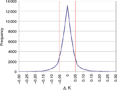
For this case study, the Bureau’s meteorological station at Wagga Wagga, NSW was chosen as a site representing a continental, mid-latitude location with a significant temperature range, from hot in summer to cool and cold in winter. One-minute data covering the midsummer month of January 2016 were analysed first, with the 5-value mean of air temperature calculated as noted above, then subtracted from its central T59 value to yield for each minute the difference (Δ) between T59 and the alternative 5-value average. Figure 2 depicts the frequency distribution of the more than 44 000 1-min Δ data points produced.
|
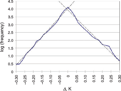
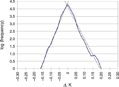
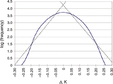
The distribution is clearly not a Gaussian or normal distribution which might be anticipated if the difference (Δ) simply reflected random error. In fact, the distribution is reasonably well approximated by a log–linear relationship, in which log of frequency is proportional to a ±Δ, as shown in Fig. 3. This is not unexpected, as will be discussed later.
|
3.3 Case 2: Wagga Wagga (Station 072150) July 2016
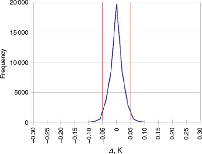
A comparable analysis for Wagga Wagga for the midwinter month of July 2016 is presented in Fig. 4 and 5. It shows a comparable, though significantly narrower probability density function (PDF) for the 44 000 values of Δ calculated for July 2016, compared to the values calculated for January (Fig. 2), which translates to approximately double the size of the log(frequency) exponents derived from Fig. 5 in comparison with the exponents derived for July from Fig. 3.
|
|
3.4 Statistical properties of Δ
Before moving on to consider any implications for T measurement of the difference (Δ) between representation of 1 min ‘instantaneous’ data by T59 compared with the 5-value average (Fig. 1), it is useful to consider the statistical character of Δ.
First, it is worth noting that although T59 is quantised to 0.1 K resolution (Δ) composed of an average of five such numbers, is quantised to one fifth that value or 0.02 K resolution, which is advantageous as it yields a smoother probability distribution function at that resolution over just a few tenths of 1 K (Fig. 2 and 4).
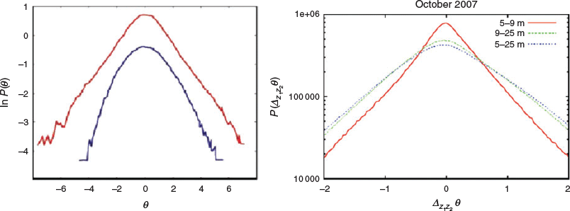
Second, the non-Gaussian, power-law form of Δ evident from Fig. 3 and 5 suggests that Δ represents temperature fluctuations driven by atmospheric turbulence, rather than random noise such as instrument noise. Under the right conditions of turbulence structure and intermittency, temperature fluctuations having this form have been studied in the time domain at a single point, for example see Shraiman and Siggia (2000). They are also found in the space domain through two-point equal-time studies of atmospheric temperature fluctuations such as in the work of Costa Frola et al. (2014). Figure 6 reproduces figures from those works showing examples of measured temperature frequency distributions exhibiting a form akin to that found here in Fig. 3 and 5.
|
Third, it was suggested in Section 3.1 that calculation of a 5-value average T centred on the last second of the minute (T59) should lead to an unbiased estimate with respect to T59 irrespective of any small secular trend in T across adjacent minutes. To check for bias, mean and median values of Δ were calculated for the full 1-s data sets from January and July at Wagga Wagga. There was no indication of significant bias, with the January mean and median values for Δ being −0.001 and 0.000 K, and the July values −0.0005 and 0.0000 K respectively. To check for any evidence of secular trend, the 44 000 values of Δ for each month were tested for correlation with the difference between T59i + 1 and T59i − 1 that would define any trend across the 2-min interval centred on T59i. Coefficient of determination values of 0.00013 and 0.00016 were found respectively for the January and July data sets.
Fourth, given the second point above that Δ exhibits statistical characteristics having a form consistent with that of scalar turbulence fields in the planetary boundary layer, and it is well known that turbulent kinetic energy in the boundary layer is driven by the diurnal cycle in solar heating (e.g. Svensson et al., 2011, see their figure 8), the two monthly Δ data sets were investigated for diurnally driven and seasonally driven behaviour.
The first test was by visual inspection of each time series over the 31 days of each of the two months, which revealed strong visual evidence in the summer (January) data set of enhanced Δ variability during daylight hours, and a very much weaker, but still discernible, increase in daytime variability of Δ in the winter (July) month. These results are illustrated by the 24-h time series of the 1-min Δ data for 17 January and 14 July presented in Fig. 7.

|
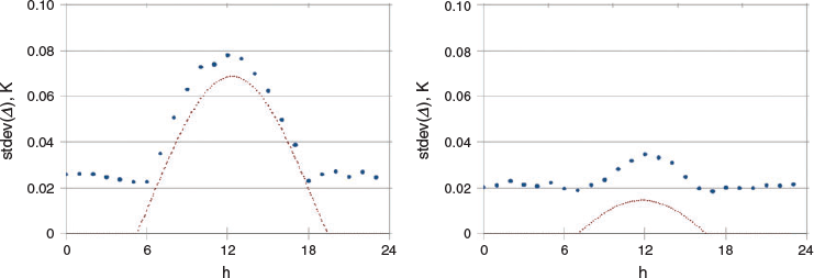
Given this initial evidence, the monthly data were sorted into 24 subsets, one for each hour in the day. The standard deviation of Δ for each 60 min was calculated then plotted against hour to reveal the diurnal cycle in variability (Fig. 8).
|
Figure 8 also contains diurnal plots of theoretical clear-sky solar irradiance onto a horizontal surface at Wagga Wagga for the middle day in each month. The evidence from Fig. 7 and 8 is compelling: Δ has a distinct diurnal cycle in variability that is well explained as being driven by the diurnal cycle in turbulent kinetic energy in the planetary boundary layer having its origin in the diurnal (and seasonal) cycle in solar irradiance at Wagga Wagga. The fact that the overnight values of hourly standard deviation in Δ are virtually the same in summer and winter and constant near a value of 0.02 K is consistent with a comment made earlier than like T, Δ is quantised, but in this case to a lower limit of 0.02 K rather than 0.1 K.
These considerations suggest that there is physically reasonable information content in the derived variable Δ, which is calculated as the difference between the 1-s air-temperature value logged by the AWS at the final second each minute and an average value of T for that same second based on that same T59 value combined with the two Tmin and two Tmax values also logged in the 2 min within which T59 sits as the central value. However, as detailed in the next section one additional test was undertaken to confirm this conclusion.
3.5 Synthetic data test – Gaussian deviates
The logarithmic PDF of temperature fluctuations observed by Costa Frola et al. (2014) (see Fig. 6) was found by the authors to be consistent over more than 12 months of continuous, 24-h observations. Its analysis led them to state that ‘The first point arising from our analysis is that the PDFs of temperature fluctuations are strongly non-Gaussian’ (top of their p. 105). To test this conclusion a synthetic data set of 2 678 400 data points was constructed representing 1 month of continuous, 24-h 1-s observations. Each point was drawn randomly from a Gaussian distribution having zero mean and standard deviation of 0.08, approximating the noontime observed value for the standard deviation of Δ in January 2016 (Fig. 8). The minimum, maximum and final value of these Gaussian deviates within each set of 60 data points were then selected to yield a synthetic 1-min data set mimicking Tmin, Tmax and T59. This data set was processed exactly as for the January/July 2016 data sets from Wagga Wagga to yield the properties of Δ that would result from Gaussian random measurement error or ‘noise’.
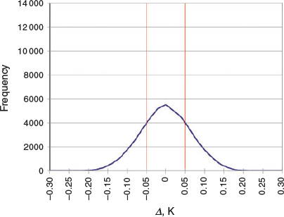
Figure 9 shows the time series of Δ over a synthetic 24-h period. Visually it is comparable with the daytime January series in Fig. 7. Figure 10 shows the frequency distribution in linear form as for Fig. 2 and 4, whereas Fig. 11 shows it in logarithmic form as for Fig. 3 and 5. Consistent with Costa Frola et al. (2014), this test shows that Δ derived from the observed 1-min AWS data cannot be attributed to Gaussian error or noise, supporting the conclusion in the section above that variability in Δ arises from real air temperature fluctuations driven by turbulence in the planetary boundary layer.

|
|
|
3.6 Synthetic data test – effect of measurement system time constant
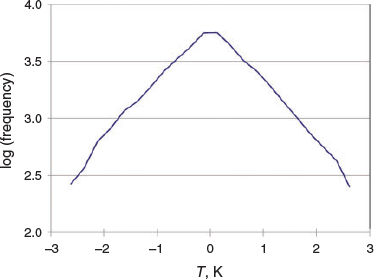
A second test involved the production of another synthetic data set of 2 678 400 data points representing each second of a 31-day month, but this time approximating the statistical properties of the measured air-temperature data set from Costa Frola et al. (2014), shown in the red line in Fig. 6. Random values were produced within bins of width 0.1 K approximating the logarithmic frequencies per bin taken from the October 5–9-m data in Fig. 6. The resultant synthetic air-temperature data set had the PDF shown in Fig. 12.
The ordinate θ used by Costa Frola et al. (2014) is air temperature normalised by the variance of the fluctuations. For the synthetic data set produced here, the values were all rescaled to approximate actual air temperature using an assumed variance value of 0.4, derived from the January Wagga Wagga data set by subtracting a 60-point running mean from each 1-min value and calculating the standard deviation of the resultant 1-min fluctuations in the deviations from the hourly means. It is important to acknowledge that the purpose here is not to try and objectively reproduce the Wagga Wagga data but simply to provide a plausible, synthetic, 1-s data set covering a 31-day month in order to investigate the effect of different measurement time constants on representations of 1-min air-temperature data using 1-s recorded values as carried out by the Bureau.
|
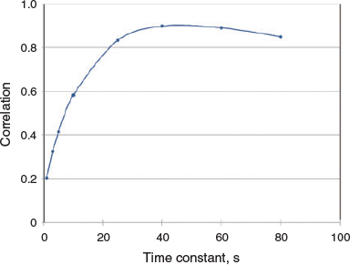
This rescaled synthetic data set representing instantaneous 1-s air-temperature fluctuations was then convolved with eight different first-order time constants representing measurement system e-folding response times ranging from 1 to 80 s. These representations of ‘measured’ data that would result from measurement systems having these eight different time constants were then processed in the same manner as the normal Bureau method to yield 44 640 1-min values for T59. A 1-min (60 s) arithmetic average (Tave) centred on T59 was calculated for comparison.
Figure 13 shows a selection of results for a randomly chosen 180-min period within the synthetic month of data. The figure compares T59 data from series subjected to four of the different measurement system time constants with the coincident 60-s average centred on T59, Tave. It is evident that, as expected, the variability in T59 decreases as time constant increases. At a time constant of 40 s, there is little difference between this smoothed representation of the 1-s T59 value and the 60-s arithmetic average centred on T59. A plot of the correlation between T59 and Tave for all eight of the time constants tested is shown in Fig. 14.
|
The Bureau has asserted with regard to its recording of 1-s data rather than 1-min averages that ‘each one second temperature value is not an instantaneous measurement of the air temperature but an average of the previous 40 to 80 seconds’ (Bureau of Meteorology 2017). The synthetic data test carried out above strongly supports that assertion. Figure 14 in particular demonstrates that in this test the correlation between T59 and the 60-s average (Tave) is very high for any time constant in the range 40–80 s, sitting at 0.9 for the 40-s time constant. In practical terms, those examples reveal no significant difference between 1-min data recorded as either T59 or Tave.
4 Implications
The aim here was to identify any difference in air temperature recorded by a Bureau AWS at 1-min intervals using the temperature measured in the last second of the minute (T59) compared with an average temperature obtained taking the mean of that value plus the two values of Tmin and Tmax recorded in the minute either side of T59. Frequency distributions of that difference (Δ) were determined using data from the Bureau’s Wagga Wagga AWS for January and July 2016.
Before considering the results it is important to note the important boundary condition that air temperature data are recorded and reported to a resolution of 0.1 K. Thus any Δ value within the range of 0 ± 0.05 K will not lead to any difference between the T59 value and the 5-value mean as no value lying within that range would be rounded up or down by 0.1 K for reporting purposes. Analogously, all values of Δ lying between +0.05 and +0.15 K would be rounded down to +0.1 K, and values between +0.15 and +0.25 K would be rounded up to +0.2 K for reporting purposes.
In that context, the July 2016 data in Fig. 4, 7 and 8 show that there would be minimal difference in moving from 1-s data to the 5-value average, because only 1.7% of Δ values (less than 1 in 50) lie above +0.05 K and 0.5% (only 1 in 200) lie below −0.05 K (the red lines in Fig. 4). The effect even in these very infrequent cases would be limited to a 0.1 K difference in recorded temperature, because only 0.027% of these Δ values lie above 0.15 K and 0.005% below −0.15 K.
Those statistics are reflected in the low values of standard deviation shown in Fig. 8 across the diurnal cycle, close to 0.02 K and well below the 0.05 K needed for rounding up or down. Night-time values close to 0.02 K are reproduced at virtually the same levels in the January standard deviation data as in the July data in Fig. 8, so even in midsummer the night-time air temperatures recorded as the last second of each minute or as a 5-value mean would be essentially identical. The implication is that Tmin would be unaffected at any time of year by taking the 5-value average rather than the 1-s value, because Tmin occurs at night-time or very early in the morning when the standard deviation of Δ is close to 0.02 K.
The enhanced variability in Δ through the middle part of the day in summer (Fig. 8) suggests a possibility of a systematic difference in temperature recorded as a 1-s value compared with a 5-value mean during that part of the day in the hottest months. The frequency distribution of Δ for January 2016 (Fig. 2) has 6.9% of values in the range 0.05–0.15 K (with just 0.9% higher) and 8.3% of values in the range −0.05 to −0.15 K (with just 0.5% lower). These numbers are small. However, these are a 24-h average and although variability overnight in Δ is small, it is large during the period of maximum solar irradiance around midday (Fig. 8). Thus a second analysis was done restricted solely to the hour between 1200 and 1300 hours local time to explore the variability in Δ at the time of maximum daily solar irradiance. The resultant frequency distribution is compared with that for all January data in Fig. 15.
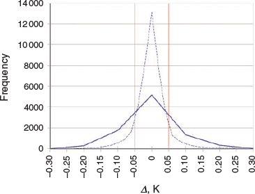
|
The distribution of Δ for the midday hour has 15% of values between 0.05 and 0.15 K and 3% above that level, suggesting that just under 1 in 5 of the T59 1-s values at midday may be enhanced by 0.1 K by turbulent variability above the comparable 5-value mean. If this applied to Tmax, on an individual daily basis this could possibly imply a one in five chance of enhancement by ~0.1 K. The implication for the climatology of Tmax, which is based on the monthly mean average of daily Tmax values, is unclear. The weighted mean effect at the time of maximum hourly variability, 1200 to 1300 hours for the July data, from the positive branch of the PDF in Fig. 14, is 0.056 K. This is marginal in terms of the rounding up requirement for Δ to exceed 0.05 K given that Tmax often occurs somewhat later in the day when variability is less than at midday (Fig. 8).
The interim conclusion is that overnight all year and all day in the cool part of the year, the difference between a 1-s T59 value and its comparable 5-value mean rarely, if ever, falls outside the range of ±0.05 K that necessary for the 1-min value to be rounded up or down by 0.1 K. If this were replicated for Tmin all year and for Tmax in the cooler months, there would be no effect on climatology, as a very rare change by ±0.1 K of a daily Tmax of Tmin would not affect discernibly the monthly means on which climatology is based, which like all T values also is quantised to 0.1 K resolution.
However, at the time of maximum T variability at noon in midsummer, the analysis suggests a marginal possibility that Tmax might be affected to some degree if the T59 result applied to Tmax: for T59 at midday turbulence led to almost one in five T59 values sitting >0.05 K above the comparable 5-value mean, so would be rounded up 0.1 K. It is not clear though that this would translate to a significant effect on climatology of Tmax, which is represented by the monthly mean of 30 daily Tmax values. To explore this further, a third case study was undertaken to consider Tmax and Tmin explicitly, rather than T59.
One other, more general implication also follows from this work. No matter what form of signal averaging is used to record the 1-min ‘instantaneous’ data as sought by the World Meteorological Organization (the Bureau’s method, the US National Weather Service method, the UK Meteorological Office method, others) the 1-min data will always exhibit more variability during daytime than at night due to the daytime solar-driven boundary layer turbulent kinetic energy: and the enhanced daytime variability will always be largest in summer.
5 Tmax and Tmin case study: September 2017 at Mildura AWS
This additional case study considers the month of September 2017 at the Bureau’s Mildura AWS (Station 076031). These station and month were chosen because of public criticism of the record made in a well-known climate change sceptic blog:
The issue of whether temperature measurements from Mildura are legitimate – or not, is relevant to every maximum and minimum value recorded at Mildura for the last 21 years. [see http://jennifermarohasy.com/2017/09/faux-record-hot-days-including-mildura/, verified 21 April 2020].
The basis for the criticism is the assertion that the 1-s Tmax and Tmin values are likely not comparable with 1-min averages, thereby overstating the maximum and minimum values recorded. As noted above the T59 analyses provide no support for this hypothesis in the case of Tmin at any time of year. However, possibility of a small effect on Tmax in midsummer was identified due to the greatly enhanced turbulent variability in T at the annual maximum of solar irradiance, which drives the midday maximum in turbulent kinetic energy in the planetary boundary layer. It is important to note though that in Section 3.6 it was found that for 1-s measurements using a 40–80-s time constant T59 already represents a 1-min arithmetic average, so averaging further such as by taking a 5-value mean would not be appropriate. Averaging an average would damp response, making it slower than the World Meteorological Organization’s required 1-min ‘instantaneous’ data. However, exploring that point quantitatively is beyond the scope here.
To investigate directly, any difference between 1-s and 1-min average values for Tmax and Tmin requires averages centred on the minute, not centred on the last second of the minute (T59) as in the case of the 5-value means used in previous sections. From Fig. 1 it is evident that for any minute, i, a 4-value mean centred on that minute can be calculated in analogous fashion as the mean of T59i−1, T59i, Tmaxi and Tmini (see Fig. 1).
To calculate the values of Tmax and Tmin based on that average then requires an estimate of the relevant deviations in T above or below that mean, which we can represent by the additional average ±(Tmaxi − Tmini)/2. We can then define difference values Δmax and Δmin as the 1-s Tmax and Tmin values minus the calculated values based on the 4-value means plus or minus the averaged max/min deviation. The frequency distributions of Δmax and Δmin are shown in Fig. 16.
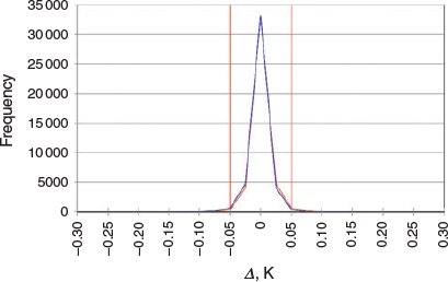
|
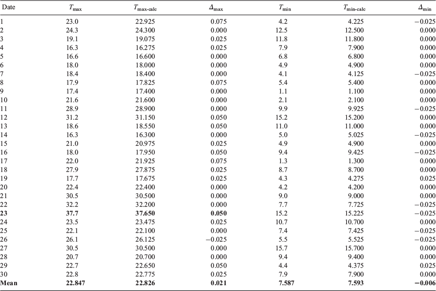
These frequency distributions are very narrow, with only 1.4% of values for each of Tmax and Tmin lying outside the ±0.05 K boundary that would see the values rounded up or down, or a 1 in 70 occurrences. To test explicitly whether such rare occurrences affected the September 2017 monthly climatology at Mildura, Table 1 contains the daily values of Tmax and Tmin recorded by the Bureau, the comparable calculated values based on the 4-value 1-min means, and the differences, Δmax and Δmin. Although the monthly mean of the 1-min Tmax values is biased slightly upwards compared with the value calculated from the 4-value 1-min averages (for reasons summarised in the next section), the difference is only 0.021 K. The recorded monthly mean Tmax is unaffected, with both the Tmax monthly mean of 22.847°C and its 4-value average counterpart of 22.826°C rounding down to the official Tmax monthly mean of 22.8°C.
For Tmin the difference between the monthly average based on 1-s data and that based on the 4-value average is much smaller, only six one-thousandths of 1 K, and both values round up to the same value at the reporting resolution of 0.1 K. This behaviour was expected based on the earlier T59 analyses that temperature fluctuations in the 1-s data are very small overnight in the absence of daytime solar-driven turbulence in the planetary boundary layer.
One other point can be made with reference to the Tmax value in Table 1 for 23 September. The Bureau’s identification of this value as a new September record stimulated the public criticism asserting the Mildura record to be probably biased high. As shown in Table 1 the 1-s Tmax value is slightly higher than the 4-value average for that minute, but not sufficiently to change the value of Tmax recorded at the 0.1 K reporting resolution of all temperature data: the calculated Tmax value rounds up in both cases to the same value of 37.7°C recorded by the Bureau, so the reported value is not biased high.
6 Further remarks
The purpose here has been to investigate the difference in 1-min air-temperature values recorded at Bureau AWS sites by 1-s measurements, compared with values averaged over the minute. Although the Bureau does not record individual 1-s values for each minute, it was possible to calculate 5-value averages centred on the last second of each minute using that value and the two sets of 1-s Tmax and Tmin values that are recorded during the minute on each side of that value. It was also possible to calculate a 4-value average centred in the middle of each minute by taking the minute’s Tmax and Tmin values and averaging those with the last second value at each end of that minute.
These representations of a 1-min average are similar to the UK Meteorological Office’s use of four measurements per minute, at 15-s intervals, for calculation of its 1-min values (UK Meteorological Office 2010). Averaging in this way acts as a very simple low-pass smoothing filter that clips some higher frequency variability from the signal. An empirical demonstration of this is provided by the synthetic data test in Section 3.5 in which Gaussian noise with zero mean and standard deviation of 0.0800 was generated to mimic 1 month of 1-s data. This was then processed to produce synthetic 1-min data for T59, Tmax and Tmin for analysis in the same way that the measured January and July 2016 AWS data from Wagga Wagga were analysed. The 5-value 1-min means from the synthetic data returned the same zero mean as the original 1-s data, but with standard deviation reduced from 0.0800 to 0.0649. The variable Δ used in the analyses above reflects precisely that effect by which extreme components of variability are filtered out by the simple multi-point smoothing filter.
That the differences between the individual 1-s data and the 4- and 5-value means are small is consistent with the Bureau’s statement that the AWS temperature measurement system has time constants built into it that already average out air-temperature fluctuations on the time scale of seconds, such that ‘each one second temperature value is not an instantaneous measurement of the air temperature but an average of the previous 40 to 80 seconds’ (Bureau of Meteorology 2017). The synthetic data test in Section 3.6 evaluating the effect of different measurement system time constants strongly supports and affirms that statement. Thus, taking a 4-or 5-point average on this type of already-smoothed data would not be expected to produce big differences, and as found. One possible flow-on implication that is beyond the scope of this work is that such further averaging of the Bureau’s already smoothed T59 data might possibly lead to over-damping of measurement system response in comparison with the time response of liquid in glass thermometers, in which case the climatological record would be biased by too much averaging rather than not enough.
7 Summary and conclusions
Comparisons were made between 1-min AWS air-temperature data recorded from a single 1-s data point or calculated as the average of four or five such values recorded in the minute, using data from Wagga Wagga (NSW). At all times of day in winter and overnight in all months 1-s values and 4- or 5-point average values did not differ significantly at the 0.1 K resolution of air temperature data. Thus Tmin values derived either way prove to be equivalent at all times of year.
For air temperature at midday in midsummer the possibility of a difference at the 0.1 K level somewhat less often than 1 min in five was identified in the January data set analysed. However, translation of this potential difference into an effect on climatological data for Tmax in midsummer was unclear, as monthly mean climatological values average over 30 days which reduces the effect of occasional individual 0.1 K difference on the mean, which also reports at only 0.1 K resolution.
This matter was explored explicitly in a case study for the month of September 2017 at Mildura for which a daily Tmax record of 37.7°C had been reported. A small mean bias of 0.021 K was found in monthly mean Tmax calculated from the daily 1-s values for Tmax compared with using 4-point averaged 1-min daily values, but this is too small to affect the reported monthly mean. At the reporting resolution of 0.1 K, both records had the same monthly mean of 22.8°C. Similarly, there was no bias in the individual daily Tmax value of 37.7°C on 23 September 2017, as this also was the same for both records at 0.1 K resolution. For Tmin the negative bias in the monthly mean from the 1-s data was negligibly small compared with the 4-point averaged data, −0.006 K, consistent with the conclusion reached earlier that overnight T measurements all year round are equivalent using either method at a resolution of 0.1 K.
The overall conclusion is that the climatology of air temperature measured by the Bureau’s AWS stations using its existing measurement methodology is not at risk of bias by recording a 1-s value to represent 1-min averages. Given the Bureau’s report that ‘each one second temperature value is not an instantaneous measurement of the air temperature but an average of the previous 40 to 80 seconds. This process is comparable to the observation process of an observer using a “mercury-in-glass” thermometer’ (Bureau of Meteorology 2017), this is unsurprising. The Bureau’s statement connotes a smoothing of atmospheric temperature fluctuations with a measurement system time constant of several tens of seconds, so 1-s data are already smoothed at the 1-min scale, as required (World Meteorological Organization 2014). This was confirmed independently by numerical evaluation of the role played by measurement system time constant using synthetic air-temperature data, which showed that a measurement system with 40–80-s e-folding time constant yields data that are very similar to that from a 60-s arithmetic mean.
Thus applying additional within-minute multi-point smoothing can only have limited effect, as found in the three-case studies and confirmed independently in the numerical test on synthetic data. Moreover, if such smoothing added additional signal damping that slowed AWS time response to less than that of traditional liquid in glass thermometers that would be undesirable in terms of historical data record equivalence. Although the conclusions reached here are not equivocal, for completeness the Bureau could consider a field experiment recording data every second to confirm directly that AWS 1-s data recorded for each minute are already representative of a once per minute measurement as required by World Meteorological Organization.
References
Bureau of Meteorology (2017). Fast facts: how does the Bureau measure temperature?, Sep. 2017: Available at http://www.bom.gov.au/inside/AWS_Review_Fast_Facts.pdf [Verified 20 April 2020].Costa Frola, E. C., Mazzino, A., Cassola, F., Mortarini, L., and Ferrero, E. (2014). An experimental study of the statistics of temperature fluctuations in the atmospheric boundary layer. Bound-layer Met 150, 91.
| An experimental study of the statistics of temperature fluctuations in the atmospheric boundary layer.Crossref | GoogleScholarGoogle Scholar |
National Weather Service (2014). Requirements and standards for NWS climate observations, National Weather Service Instruction 10-1302. (National Oceanic & Atmospheric Administration, Department of Commerce: USA.)
Shraiman, B. I., and Siggia, E. D. (2000). Scalar turbulence. Nature 405, 639.
| Scalar turbulence.Crossref | GoogleScholarGoogle Scholar |
Svensson, G., Holtslag, A. A. M, Kumar, V., Mauritsen, T., Steeneveld, G. J., Angevine, W. M., Bazile, E., Beljaars, A., De Bruijn, E. I. F, Cheng, A., and Conangla, L. (2011). Evaluation of the diurnal cycle in the atmospheric boundary layer over land as represented by a variety of single-column models: the second GABLS experiment. Bound-Layer Met 140, 177.
| Evaluation of the diurnal cycle in the atmospheric boundary layer over land as represented by a variety of single-column models: the second GABLS experiment.Crossref | GoogleScholarGoogle Scholar |
UK Meteorological Office (2010). National meteorological library and archive fact sheet 17 — weather observations over land. (UKMO: Exeter UK.)
World Meteorological Organization (2014). Guide to meteorological instruments and methods of observation (WMO-No. 8). (WMO: Geneva, Switzerland.)


