
Spatiotemporal energetics analysis of Deep Western Boundary Current eddies at 11°S, off north-eastern Brazil
André Lopes Brum A * and José Luiz Lima de Azevedo A
A
Abstract
The three-dimensional energetics of deep mesoscale eddies is investigated in a time-dependent theoretical framework using 36-year output of a 1/10° eddy-resolving ocean general circulation model. Composite analyses are conducted based on 29 anticyclonic eddies in the Deep Western Boundary Current (DWBC) at 11°S. The DWBC constitutes a key component of the lower limb of the Atlantic Meridional Overturning Circulation, crucial for comprehending climate change dynamics. Energetics analyses reveal that within the DWBC isolated eddies, advection is the main source of eddy kinetic energy (EKE) and eddy potential energy (EPE). Near the coast, energy conversion terms show that the anticyclones drain energy from the mean DWBC, enhancing the eddy field. Depth-integrated analysis found direct and inverse energy cascades within the average DWBC eddy with similar magnitude and area coverage size. The eddy–mean flow interaction terms were analysed in an Eulerian frame of reference along the eddy area, depicting their variability while migrating at a fixed point. Overall, direct energy cascade dominates the barotropic energy conversions during eddy migration, with enhanced conversion rates associated with peaks of eddy velocity. By contrast, the baroclinic energy conversions presented alternate direct-inverse energy cascades during eddy migration. At the eddy core depth, the barotropic (baroclinic) energy pathway contributes to the growth (decay) of EKE (EPE) at a rate of ~1.0 J m−3 day−1 (5.4 × 10⁻⁶ J m−3 day−1). This study seeks to extend our knowledge of the energy budgets within deep mesoscale eddies, a key factor for understanding ocean dynamics and circulation.
Keywords: baroclinic instability, barotropic instability, deep mesoscale eddies, Deep Western Boundary Current, eddy kinetic energy, eddy potential energy, eddy–mean flow interactions, growth rate, time-dependent framework.
1.Introduction
The Deep Western Boundary Current (DWBC) is a main component of the Atlantic Meridional Overturning Circulation (AMOC) lower limb, transporting North Atlantic Deep Water (NADW) from the North Atlantic to the Southern Ocean along the western edge of the Atlantic Basin (e.g. Rhein and Stramma 2005; Schott et al. 2005; Lumpkin and Speer 2007; Garzoli et al. 2015). In the northern subtropical Atlantic, the DWBC flows as a coherent jet (Bower et al. 2009; Gary et al. 2011), although observations (e.g. Lee et al. 1996) and models (e.g. Lüschow et al. 2019) suggest strong temporal variability of the DWBC associated with meanders and eddies. In the tropical Atlantic, Schott et al. (1993) observed a well-established shallow DWBC (1000–2500-m depth) flowing south-eastward from 44 to 35°W, where a deep DWBC limb incorporates the eastward flow with a core velocity guided by the Parnaiba Ridge at 1°45′S (Rhein et al. 1995; Schott et al. 2003).
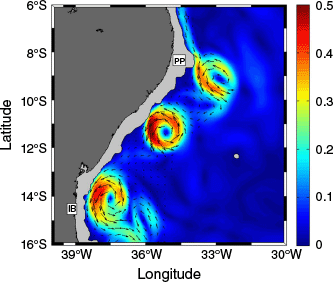
Along the Brazilian continental slope, the DWBC is re-established as a continuous flow near 5°S at depths of 1200–4000 m (Schott et al. 2003, 2005). At 11°S, moored velocity records showed enhanced variability with periods of 60–70 days near 2000-m depth, characterised as anti-cyclonically rotating coherent vortices (Fig. 1), responsible for the poleward transport of NADW at the western boundary (Dengler et al. 2004). The authors also described these eddies translating south-westward along the continental slope with an average alongshore velocity of 4 cm s−1, maximum azimuthal velocity that can exceed 20 cm s−1, an e-folding radius and height of 60 and 1070 m respectively, and with core depth near 2000 m.
Snapshot of horizontal velocity amplitude (colour-coded, m s−1) and vectors (black arrows) at 1900-m depth from Ocean General Circulation Model for the Earth Simulator (OFES). The light grey areas represent regions shallower than 1900-m depth. The Pernambuco Plateau (PP) and Ilhéus Bight (IB) are indicated.
The DWBC eddy generation area near 8°S was first described by Dengler et al. (2004) using results from a Family of Linked Atlantic Model Experiments (FLAME) model, indicating the influence of the meridional overturning circulation in eddy generation. The Lüschow et al. (2019) snapshots from the STORM/NCEP simulation reveal nearly vertically coherent, topographically controlled eddies propagating southward alongshore across the full depth range of the DWBC near 11°S. More recently, Vilela-Silva et al. (2023) proposed the intermittent separation of the DWBC from the boundary while contouring the Pernambuco Plateau (~8°S) as a potential eddy formation mechanism, with 4.5 ± 0.5 anticyclones being released per year.
At the south of 13°S, Brum et al. (2023) used output of the Ocean General Circulation Model (OGCM) For the Earth Simulator (OFES) and found that the eddies strongly interact with a quasi-stationary eddy centred at 14.5°S within the Ilhéus Bight area, and that the DWBC re-establishes as a continuous flow south of 17°S. Therefore, mesoscale activity has a strong impact on the DWBC’s advective timescale and plays a key role in the circulation and variability of the AMOC lower limb.
Mesoscale eddies contribute to the global oceanic energy budget and are responsible for substantial mass and heat transport, thus playing a key role in the global climate system. Additionally, these features play a crucial role in energetically driving eddy–mean flow interactions and associated instability processes (e.g. Napolitano et al. 2019; Brum et al. 2023; Vilela-Silva et al. 2023). Works including energy budgets are mostly performed on a time-mean basis, such as the climatological mean (e.g. Cronin and Watts 1996; Von Storch et al. 2012; Chen et al. 2014; Kang and Curchitser 2015; Brum et al. 2017; Magalhães et al. 2017; Yan et al. 2019) and the bandpass running mean (e.g. Jouanno et al. 2012; Kang et al. 2016; Brum et al. 2023). The time-dependent perspective was first introduced by Chen et al. (2016) and has been successfully applied to investigate the variability of mesoscale eddies (e.g. Yan et al. 2022) and meanders (e.g. Yamagami et al. 2019). Hence, a better description of these features is a key factor for understanding ocean dynamics and circulation.
Most studies of mesoscale eddies focus on their interaction with boundary currents (e.g. Chern and Wang 2005; Yan et al. 2022) or on the spatiotemporal variability of eddy properties (e.g. Yang et al. 2013; Zhang et al. 2020). In the Kuroshio Current, results from Geng et al. (2016, 2018) indicate that advection and pressure work can play important roles in eddy decay, and that eddy kinetic energy (EKE) and eddy potential energy (EPE) decrease with depth and time. Jan et al. (2017) performed six numerical experiments and found that, in addition to eddy polarity, the eddy strength and impinging latitude exert important effects on the eddy evolution. Using model outputs to analyse the energetics of the eddy–Kuroshio Current interaction, Yan et al. (2022) observed EKE (EPE) peaks at the eddy boundary (centre). Nevertheless, the energy conversion pathways within individual eddies require further investigation.
Although energetics analysis has mainly focused on near-surface currents, EKE budgets in the lower-layer western boundary of the South Atlantic Ocean have been increasingly studied. At a moored array near 11°S, Dengler et al. (2004) observed EKE levels of ~50 cm2 s−2 from the 50- to 90-day band-pass filtered velocity time series. At the same moored position, Schott et al. (2005) observed mean EKE values of 70–150 cm2 s−2 within the DWBC layer depth. Eddy-resolving OGCMs also found enhanced EKE at deeper levels near the western boundary off north-east Brazil (e.g. Garzoli et al. 2015; Lüschow et al. 2019; Brum et al. 2023; Vilela-Silva et al. 2023). Garzoli et al. (2015) indicated elevated levels of EKE spreading further offshore south of 8°S, consistent with the formation of DWBC eddies. Average EKE levels of 40–70 cm2 s−2 were found by Lüschow et al. (2019) in the DWBC off north-east Brazil at 1941-m depth, whereas Brum et al. (2023) showed average values of EKE of 50–250 cm2 s−2 along the north-eastern Brazilian coast at 1900-m depth. Additionally, Brum et al. (2023) and Vilela-Silva et al. (2023) found that barotropic instabilities are the primary source of EKE in the region, contributing to eddy generation and propagation.
In addition to the eddy–mean flow interaction in the DWBC off north-east Brazil, the spatiotemporal variability of the energy conversion pathways within the individual eddies requires further investigation. In this contribution, we investigate the temporal evolution and three-dimensional average structure of the energy budgets and conversion terms within the DWBC eddies at 11°S. Our analysis is based on 36 years of output from an eddy-resolving 1/10° OGCM. Section 2 describes the model output and methods used. The results of the energetics analysis of the DWBC eddies are presented in section 3, whereas section 4 provides concluding remarks.
2.Data and methods
2.1. Model output
The analyses in this study are based on output from the OFES, developed by the Japan Agency for Marine-Earth Science and Technology (JAMSTEC), spanning 36 years (1980–2015). The model is based on the third version of the Modular Ocean Model–MOM3 (Pacanowski and Griffies 2000), and it is forced by surface wind stress, heat and freshwater fluxes derived from the daily mean National Centers for Environmental Prediction–National Center for Atmospheric Research (NCEP–NCAR) reanalysis. The OFES covers the global domain from 75°S to 75°N with an eddy-resolving horizontal resolution of 1/10° on a Mercator B grid. It includes 54 vertical z-levels, with layer thickness increasing from 5 m at the surface to 330 m near the ocean bottom. The model solves the three-dimensional primitive equations in spherical coordinates by considering the hydrostatic and Boussinesq approximations. The bathymetric field is based on a 1/30° database provided by the Ocean Circulation and Climate Advanced Modelling (OCCAM) project (de Cuevas et al. 1999). Detailed descriptions of the model setup and analyses can be found in Masumoto (2010).
Here, we used snapshots at 3-day intervals of three-dimensional velocity, temperature and salinity. In accordance with DWBC observations (Dengler et al. 2004; Schott et al. 2005) and other numerical simulations (Lüschow et al. 2019; Brum et al. 2023; Vilela-Silva et al. 2023), OFES mean DWBC flow is found within the depth range of 1000–3000 m (hereafter referred to as the DWBC layer depth), with a core depth near 1900 m. The velocity data were analysed in an along- and cross-shore coordinate system by rotating zonal and meridional velocity components 36° clockwise against the north (e.g. Dengler et al. 2004; Schott et al. 2005; Hummels et al. 2015; Brum et al. 2023).
The OFES output has recently been utilised to analyse eddy–mean flow interactions (e.g. Qiu et al. 2014; Chen et al. 2015; Yang and Liang 2016; Brum et al. 2017; Yan et al. 2019, 2023; Yang et al. 2020; Zhang et al. 2021; Adeagbo et al. 2022; Liu et al. 2022) and mesoscale eddy structures (e.g. Chiang and Qu 2013; Wang 2017; Yan et al. 2022; Zhang et al. 2024) in western boundary currents.
In the vicinity of the north-eastern Brazilian continental slope, the OFES model has successfully been applied to study the structure and variability of the DWBC (e.g. van Sebille et al. 2012; Garzoli et al. 2015; Brum et al. 2023), as well as the time-mean and time-dependent components of AMOC (e.g. Dong et al. 2011; Perez et al. 2011), and eddy–mean flow interaction (e.g. Brum et al. 2023). In addition, Yan et al. (2022) used OFES output to analyse eddy–current interactions in a time-dependent framework.
Therefore, the OFES model has successfully simulated the DWBC structure, variability, eddy–mean flow interactions, and energy budgets. For a detailed evaluation of the OFES model in the DWBC off north-east Brazil, please refer to van Sebille et al. (2012) and Brum et al. (2023).
2.2. Time-dependent energy diagnostic framework
To investigate the temporal evolution in the energetics of eddy–mean flow interaction, energy densities for the eddy field are first defined. The kinetic energy variations induced by the DWBC eddies from background flow variations are isolated by defining the mean flow as a low-pass running mean (hereafter denoted by an overbar), and the eddy field as the deviation from the time mean (hereafter denoted by primes) (e.g. Jouanno et al. 2012; Rieck et al. 2015; Kang et al. 2016; Brum et al. 2023). Previous studies have shown that intraseasonal fluctuations with periods of 60–70 days are the most prominent signal in the region (e.g. Dengler et al. 2004; Schott et al. 2005; Brum et al. 2023; Vilela-Silva et al. 2023). Therefore, we used a 120-day running mean to accurately represent the DWBC eddy field in the time-varying flow and to remove other features such as seasonal signals (e.g. Brum et al. 2023). Thus, model variables are decomposed as the sum of a low-passed component and the anomaly.
Based on such eddy–mean flow decompositions and following Kang and Curchitser (2015), EKE and the linear definition of available EPE (J m–3) (Gill 1982) are given as follows:
where ρ = 1036.4 kg m−3 is the constant reference density calculated with respect to the averaged density at 1900-m depth within the study domain, and u(v) is the zonal (meridional) velocity component. The buoyancy frequency N2 is given by:
and g = 9.807 m s−2 is the gravity constant. The term ρ* represents the perturbation density related to the reference density ρr, determined by decomposing density as ρ(x, y, z, t) = ρr(z) + ρ*(x, y, z, t). The perturbation density denotes the dynamic component (spatiotemporally variable) of the reference density (averaged over time and space and constant at a given depth). Decomposing ρ* yields:
where is the temporal average of the perturbation density (related to the reference density) and is its deviation. Following the same decomposition, the pressure p is split as p = pr + p*, where pr(p*) denotes the reference (perturbation) pressure.
Based on the energy definitions above, the time-dependent EKE and EPE equations for evaluating the eddy–mean flow interaction within a fixed ocean domain can be derived. Detailed derivations of the energy equations for the mean flow and eddy field can be found in Kang and Curchitser (2015), Chen et al. (2016), Brum et al. (2017) and Yan et al. (2022). Here, the equations describing the balance of EKE and EPE are presented for ease of reference:
where u = (u, v, w) is the three-dimensional velocity vector, ∇ = (∂ ÷ ∂x)i + (∂ ÷ ∂y)j + (∂ ÷ ∂z)k = ∇h + (∂ ÷ ∂z)k is the nabla operator, and and are forcing and dissipation terms respectively. The definitions of the eddy–mean flow interaction terms related to EKE and EPE budgets are listed in Table 1. Note that MKE and MPE are the mean kinetic energy and mean potential energy respectively.
| Term | Mathematical form | Meaning | |
|---|---|---|---|
| BTC1 | −ρ1900(u′ u′ × ∇u̅ + v′ u′ × ∇v̅) | Barotropic MKE ↔ EKE conversion due to the interaction between eddy momentum fluxes and mean horizontal shear | |
| BTC2 | Barotropic MKE ↔ EKE conversion due to the interaction between horizontal eddy fluxes and eddy momentum flux divergence | ||
| BCC1 | Baroclinic MPE ↔ EPE conversion due to the interaction between eddy density fluxes and mean density gradient | ||
| BCC2 | Baroclinic MPE ↔ EPE conversion due to the interaction between perturbation density and the divergence of eddy density fluxes | ||
| VEDF | Baroclinic EPE ↔ EKE conversion through vertical eddy density flux due to the work performed by turbulent buoyancy forces on the vertical stratification | ||
| AEKE | −∇ × ( u̅EKE) | Redistribution of EKE due to advection | |
| AEPE | −∇ × ( u̅EPE) | Redistribution of EPE due to advection | |
| PW′ | Redistribution of EKE due to pressure work |
The terms BTC2 and BCC2 are associated with the eddy field. These terms vanish upon time averaging and are excluded in the time-mean energy diagnostic framework, as demonstrated in Chen et al. (2014) and Kang and Curchitser (2015). However, in the time-dependent diagnostic framework, the magnitude of these terms can significantly influence the evolution of eddies (e.g. Yan et al. 2022).
2.3. Mesoscale eddy events
The DWBC eddies were identified and tracked in the eddy migration area (~9.5–13.0°S) at 1900-m depth (the core depth of the DWBC) by analysing the horizontal distribution of velocity, EKE, relative vorticity (positive for anticyclonic eddies in the Southern Hemisphere), and closed streamlines. A total of 155 DWBC eddies were identified and tracked in 2890 snapshots spanning the 36 years of model simulation. However, most of these eddies undergo direct eddy–eddy interaction followed by merging along the migration area. Therefore, to avoid the influence of the eddy–eddy interaction in our analysis, we performed the energetic analysis exclusively on pinched-off eddies that migrated from the generation site towards 13.0°S without interacting with another eddy, termed isolated eddies in the following. South of 13.0°S, these eddies are strongly influenced by the quasi-stationary anticyclonic eddy located near 14.5°S (Brum et al. 2023). When first experiencing the dynamics of the mean flow dominated by the quasi-stationary feature, the migrating eddies exhibit reduced poleward propagation. At this point, we ended the tracking of the eddies.
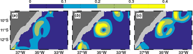
In this context, we identified and tracked 29 isolated eddies within the pathway area spanning 868 snapshots. The remaining 126 eddies were influenced by direct eddy–eddy interaction, which affects the analyses. Despite comprising ~20% of the total number of DWBC eddies, the structure and energy exchange patterns of deep mesoscale eddies (the focus of this contribution) remain preserved when analysing isolated eddies (not influenced by other interaction dynamics). By including all eddies, the study would turn to the dynamics of the interactions between eddies, which does not fit the scope of this study. Fig. 2 depicts three examples of DWBC eddies centred at 11°S: one isolated and two non-isolated.
Snapshots of horizontal velocity amplitude (colour-coded, m s−1) at 1900-m depth from the OFES. (a, c) Non-isolated eddies; (b) isolated eddy. The light grey area represents regions shallower than 1900-m depth.
Based on previous studies (Dengler et al. 2004; Brum et al. 2023), as well as model animations (not shown here), the central latitude of the migration area selected as the reference latitude for the three-dimensional analyses was 11°S. Snapshots of the OFES model velocity (Fig. 1) clearly depict DWBC eddies still attached to the upstream jet at the north of 10°S and strongly influenced by the quasi-stationary anticyclonic eddy at the south of 13°S.
2.4. Composite analysis method
To investigate the average temporal evolution and three-dimensional structure of the energy budgets and eddy–mean flow interaction terms of the DWBC isolated eddies, a composite analysis method was employed (e.g. Carranza et al. 2017; Yan et al. 2022; Vilela-Silva et al. 2023, 2024). Composite analyses are used to obtain more general conclusions, reducing noise from motions in other frequencies (e.g. Chang et al. 2015). A composite analysis was used by Yan et al. (2022) to statistically investigate the energetics processes during eddy–Kuroshio interactions east of Taiwan, whereas Vilela-Silva et al. (2023) applied composite analysis to diagnose the DWBC eddy formation mechanism.
To analyse the temporal evolution of the DWBC isolated eddies during propagation, we first defined the longitude (hereafter termed lonc) where the eddy centre (minimum velocity amplitude within the feature) is at 11°S as the fixed longitude to record the magnitude of each term (Fig. 3a). Thus, we denote position C at coordinates (lonc, 11°S). In this context, the time series represents the variation of the magnitude of each term throughout the entire migration of the eddy through position C, characterising an Eulerian frame of reference. Note that lonc varies for each individual eddy. Fig. 3 provides a schematic representation of the methodology used to construct these time series.
Schematic representation of the methodology used to construct the time series of energy terms. The black circle represents the DWBC eddy boundary, and the black arrows indicate the rotation direction. The red axes represent the meridional (y-axis) and zonal (x-axis) components, whereas the blue axes represent along- and cross-shore components. The westernmost black contour line depicts the coastline, and the blue dashed lines enclose the eddy migration pathway direction, indicated by the large blue arrow. (a) Snapshot used to identify the eddy centre at 11°S, defining position C (black dot at lonc,11°S); light (dark) green area indicates the Northern (Southern) Hemisphere of the eddy. (b) The first value of the time series (black dot) is registered when the south-western edge of the eddy reaches position C. (c) Subsequent values of the time series (marked by black dots) are recorded during the eddy’s south-westward migration through position C. (d) The north-eastern edge of the eddy crosses position C, indicating the final recorded value in the time series.
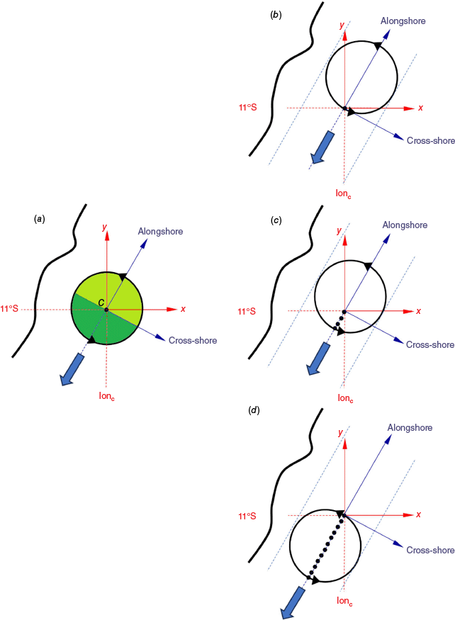
Based on the cross-shore velocity field within the eddy, the feature can be divided into two hemispheres: the Southern Hemisphere with positive (south-eastward) cross-shore velocity, and the Northern Hemisphere with negative (north-westward) cross-shore velocity (see green areas in Fig. 3a). In this context, the time series of these terms spans the entire eddy area in the alongshore direction, from the first positive cross-shore velocity value to the last negative cross-shore velocity value.
Additionally, the time axis of each eddy track was redefined: day 1 was defined as the date when the eddy’s south-western edge (first positive cross-shore velocity) reaches position C (Fig. 3b). In this context, snapshots of the terms within the eddies were obtained at position C at 3-day intervals. To create the average temporal evolution, we normalised the time series of the Southern (Northern) Hemisphere by the average duration of the 29 Southern (Northern) Hemispheres. Finally, we concatenated the normalised time series of the Southern and Northern Hemispheres to create the final averaged time series. Based on the temporal evolution of relative vorticity, we defined the positive relative vorticity area as the eddy core area.
The averaged eddy structure was generated by positioning the 29 isolated eddies at the same central position for both horizontal and vertical structure figures. It is worth mentioning that the vertical sections were not examined in the cross-slope direction because the eddy’s cross-shore velocity component is close to zero at the eddy centre along the cross-slope direction, leading to the vanishing of the related energy conversion terms. For ease of reference, we defined the eddy boundary, in the horizontal and vertical structure figures, as the outermost closed contour line corresponding to 30% of the maximum velocity amplitude, outwards of the maximum tangential velocity contour line. This definition follows previous studies (e.g. Olson 1991; Dickey et al. 2008; Nencioli et al. 2010) that demonstrated eddy velocity fields typically exhibiting minimum velocities near the eddy centre, with tangential velocities increasing with distance from the centre until reaching a maximum and then decaying. However, we emphasise that none of the eddy parameters or energy terms computed here are influenced by the choice of the eddy boundary threshold.
3.Results and discussion
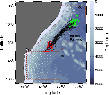
After detachment from their generation site, the DWBC eddies propagate south-westward with mean duration of 93.1 ± 18.9 days until 13.0°S. This estimate is in good agreement with Dengler et al. (2004) observations of alongshore translation velocity of ~3.8 ± 0.9 cm s−1 and Brum et al. (2023) EKE poleward phase propagation from 10 to 13°S of ~1° of latitude per month. All trajectories of the 29 isolated eddies are presented in Fig. 4. The trajectories do not end at the same latitude because each eddy interacts with the quasi-stationary anticyclonic eddy at different latitudes based on its unique structure.
Trajectories of the 29 isolated eddies (black lines). Green (red) dots denote the positions of eddy detachment (interaction with quasi-stationary anticyclonic eddy). White arrows indicate the 36-year average DWBC horizontal velocity vectors at 1900-m depth. The three labelled brown boxes indicate the areas of eddy generation (Gen), eddy migration pathway (Eddies Pathway) and the quasi-stationary eddy (QE). The colour shading represents the local bathymetry (m).
3.1. Average structure of the DWBC eddies
The energy budgets and eddy–mean flow interaction terms are computed based on the eddy velocity (u′, v′, w′) and perturbation density fields. Therefore, Fig. 5 presents the average horizontal (depth-integrated throughout the DWBC layer depth) and vertical distribution of these terms, in addition to the vertical component of the relative vorticity (ζz = ∂v′ ÷ ∂x − ∂u′ ÷ ∂y).
Three-dimensional structure of perturbation density (, kg m−3) (a, f), eddy velocity components (m s−1) u′ (b, g), v′ (c, h), w′ (d, i), and relative vorticity (s−1) (e, j) of the averaged DWBC isolated eddy, from OFES model output. Upper panels: horizontal distribution integrated vertically between 1000 and 3000 m, outermost (innermost) black contour line indicates the eddy boundary (centre). Lower panels: vertical zonal sections at 11°S, black contour lines indicate onshore and offshore eddy lobe boundary, blue and red contour lines in (f) indicate elevated values, grey areas represent bottom topography.
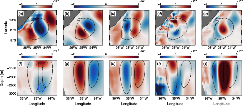
The cross-shore (u′ in Fig. 5b, g) and alongshore (v′ in Fig. 5c, h) eddy velocity components structure highlights the anticyclonic rotation (positive relative vorticity in Fig. 5e, j). Mean alongshore velocity in the coastal (oceanic) lobe was ~0.20 ± 0.07 m s−1 (0.16 ± 0.06 m s–1). This asymmetry was first observed by Dengler et al. (2004) and further by Schott et al. (2005). These studies used lowered ADCP data and a moored array at 11°S to present mean alongshore velocities and transport estimates in the coastal lobe twice as large as in the oceanic lobe. However, the 120-day running mean used in his study removes the variability of the background flow, decreasing our estimate of the alongshore component mainly related to the coastal lobe. Krelling et al. (2020) also observed the asymmetric signature of the DWBC anticyclone at 9°S. Additionally, observations in Vilela-Silva et al. (2023) revealed an asymmetry between the coastal and oceanic lobes. However, the authors suggest that the observed DWBC maximum velocities are at least 1/3 smaller than previous studies (e.g. Dengler et al. 2004; Schott et al. 2005; Krelling et al. 2020), possibly due to the coarse spatial resolution between hydrographic stations.
Depth-integrated horizontal distribution of the eddy vertical velocity (w′ in Fig. 5d) indicates downwelling (negative w′) in the Southern Hemisphere and upwelling (positive w′) near the coast in the Northern Hemisphere. However, the vertical structure of w′ (Fig. 5i) showed opposite patterns between the coastal and the oceanic lobe: within the coastal (oceanic) lobe, eddy vertical velocity presented upwelling (downwelling) above the core (~2000 m) and downwelling (upwelling) below the core. By using an overturning streamfunction describing the time-mean flow in the plane normal to the DWBC near 11°S, Lüschow et al. (2019) found downwelling of eddy density fluxes close to the shore and upwelling further offshore.
Furthermore, the horizontal structure of perturbation density ( in Fig. 5a) shows positive–negative alongshore variability with elevated negative values around the eddy centre. Its vertical distribution (Fig. 5f) depicts a first-mode baroclinic structure with a local maximum in the upper layer, also found by Lüschow et al. (2019).
3.2. Average temporal evolution
The Eulerian framework is employed for the first time to analyse the temporal variability of the eddy–mean flow interaction terms within the DWBC eddies. Unlike the Lagrangian approach, which tracks the trajectory of a feature, by employing an Eulerian framework, the analysis captures the temporal evolution of energy budgets, conversion terms, velocity, vorticity and other characteristics of the eddies as they migrate through fixed locations. This is particularly useful for diagnosing the energetic impacts of oceanic features – such as mesoscale eddies – on local currents, stationary features (e.g. meanders, fronts or recirculation patterns) and even engineering infrastructure.
The average temporal evolution of the eddy properties, energy budgets and eddy–mean flow interaction terms within the isolated eddies are presented in Fig. 6. The length of the time series indicates that the average Southern (Northern) Hemisphere takes 34 (30) days to completely migrate over position C, totalling 64 days. This pattern indicates that the Southern Hemisphere of the DWBC eddies is slightly larger than the Northern Hemisphere, suggesting an alongshore asymmetry – in addition to the cross-shore asymmetry shown in Fig. 5. As expected for mesoscale eddies, the eddy core area is characterised by maximum relative vorticity (positive for anticyclonic eddies in the global Southern Hemisphere) and perturbation density (negative for anticyclones), but minimum eddy velocity (Fig. 6a).
Average temporal evolution of energy terms of the 29 isolated DWBC eddies at 1900-m depth at 11°S. (a) Eddy velocities, relative vorticity, EKE, EPE and perturbation density; (b) terms related to the balance of EKE equation; (c) terms related to the balance of EPE equation. The black horizontal (vertical) line highlights the zero (eddy centre). Grey background indicates the eddy core area (positive relative vorticity).
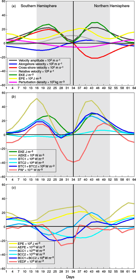
In agreement with the eddy boundary definition described in section 2.4, the eddy velocity time series show minimum values at the eddy centre that increase with distance from the centre before reaching a maximum value and then decaying (Fig. 6a). Energy budgets within the eddy core (days 16–52) are characterised by maximum EPE and minimum EKE (as in Yan et al. 2022). The EKE magnitude within the feature is consistent with previous work (e.g. Dengler et al. 2004; Schott et al. 2005; Garzoli et al. 2015; Lüschow et al. 2019; Brum et al. 2023).
Energy transfer associated with eddy momentum fluxes (BTC1, BTC2; Fig. 6b) is three to four orders of magnitude larger than that related to eddy density fluxes (BCC1, BCC2; Fig. 6c). This is expected at the eddy core depth because the potential energy budget and its exchanges are stronger in the upper and lower layers (e.g. Lüschow et al. 2019; Brum et al. 2023). Previous studies have shown that barotropic instabilities dominate over baroclinic instabilities within the DWBC. In the Northern Hemisphere, Solodoch et al. (2020) and Schulzki et al. (2021) used numerical models to reveal the barotropic conversion dominance around the Flemish Cap (~45°N) and further south (~26°N) respectively. In the Southern Hemisphere, Brum et al. (2023) and Vilela-Silva et al. (2023) found the barotropic conversion pathway one to three orders of magnitude larger than the baroclinic conversion in the vicinity of the north-eastern Brazilian continental slope. The larger magnitudes of the conversion terms (BTC1, BTC2, BCC1, BCC2 and VEDF) within the eddy core, compared with the magnitudes outside the core, indicate enhanced energy exchange in this area.
During eddy migration, maximum EKE of the most energetic isolated eddy reaches 90 J m−3 (not shown here). For the 29 isolated eddies, the average maximum EKE is ~26 J m−3 in the Southern Hemisphere and ~29 J m−3 in the Northern Hemisphere. This enhanced EKE is mainly supported by barotropic conversion, of which the horizontal shear of the background flow, measured by the term BTC1, is up to four times larger than BTC2, with extreme values being ~26.5 × 10⁻⁶ and ~6.1 × 10⁻⁶ W m−3 respectively (Fig. 6b). In this context, the average EKE growth rate due to barotropic energy pathway is ~1.0 J m−3 day−1, reaching maxima near 2.7 J m−3 day−1. By adding the advection of EKE by the mean flow (AEKE term), EKE enhances on average ~2.7 J m−3 day−1, reaching extreme values of ~6.9 J m−3 day−1 (nearly 1 J m−3 in 3.5 h).
Moreover, the eddy-induced velocity anomaly, represented by the term BTC2, is twice as large in the eddy Northern Hemisphere compared to the Southern Hemisphere. Although the temporal evolution of the BTC1 indicates constant energy conversion pathway (from the mean flow to the eddy field) in both hemispheres of the eddy during migration at 11°S, the BTC2 term indicates energy conversion pathway alternating in each hemisphere: inverse energy cascade (EKE → MKE) in the Southern Hemisphere, and direct energy cascade (MKE → EKE) in the Northern Hemisphere. Terms related to the kinetic energy budget present a peak in each hemisphere of the eddy and lower levels near the centre (consistent with the minimum tangential velocity at the centre).
Although the PW′ term exhibits a pattern similar to EKE, BTC1 and AEKE, its magnitude is four to five orders lower. Therefore, pressure work is not a prominent energy source within the DWBC eddies, as suggested by Brum et al. (2023).
Elevated EPE is observed around the eddy centre (e.g. Yan et al. 2022), consistent with the steepened isopycnal slope. The maximum EPE of the most energetic isolated eddy reaches ~0.7 J m−3 (not shown here), whereas the average EPE of the isolated eddies was ~0.2 J m−3 (Fig. 6c). Within the eddy core area, negative values of BCC2 indicate inverse energy cascade due to the interaction between perturbation density (negative around the eddy core, see Fig. 5a) and the background divergence of eddy density fluxes (positive along the DWBC eddies pathway, not shown here). By contrast, VEDF and AEPE terms indicate energy transfer to the EPE budget, with the VEDF term being one order of magnitude larger than the AEPE.
During migration at 11°S, the average DWBC eddy exhibits complex temporal baroclinic conversion pathways. In the Southern Hemisphere of the eddy (Fig. 6c; days 1–34), BCC1 indicates direct (inverse) energy cascade from MPE to EPE (EPE to MPE) near the boundary (core area). By contrast, in the eddy’s Northern Hemisphere (Fig. 6c; days 34–64), BCC1 indicates the opposite energy cascade pathway in the respective areas. Furthermore, BCC2 indicates direct (inverse) energy cascade from MPE → EPE (EPE → MPE) in the eddy boundary (core area). Therefore, the temporal evolution of eddy cross-stream velocity (u′; Fig. 6a red line) and perturbation density (; Fig. 6a pink line) indicates that the eddy density fluxes related to the cross-shore eddy velocity modulates the BCC1 temporal evolution pattern, converting energy from the mean flow (eddy field) to the eddy field (mean flow) when perturbation density and u′ are of the same (opposite) sign. By contrast, BCC2 is strongly modulated by the perturbation density pattern, converting energy from the mean flow (eddy field) to the eddy field (mean flow) when perturbation density is positive (negative). Maximum values of BCC1 and BCC2 are found in the eddy Northern Hemisphere within the core area (days 34–52) reaching ~±2.0 × 10⁻⁹ W m−3 (Fig. 6c blue lines). In this context, the average baroclinic energy conversion within the DWBC eddies is negative (inverse energy cascade) and the EPE decay rate is ~5.4 × 10⁻⁶ J m−3 day−1, with extreme values of ~1.8 × 10⁻⁴ J m−3 day−1. When computing the advection of EPE by the mean flow (AEPE term), the direct energy cascade dominates and the EPE growth rate is ~1.6 × 10⁻⁴ J m−3 day−1, reaching maximum values of ~3.8 × 10⁻⁴ J m−3 day−1. Therefore, we suggest that the effects of forcing and dissipation should be relevant for the EPE growth rate within the DWBC eddies and should be part of future studies.
The AEKE and AEPE indicate the redistribution of energy by mean flow advection and exhibit similar patterns – enhanced values before EKE and EPE peaks respectively (Fig. 6b, c respectively). These terms have the greatest influence on the EKE and EPE growth rate. The average maximum of AEKE is ~5.1 × 10⁻⁵ W m−3 (Fig. 6b), with extreme values in the most energetic eddies exceeding 2.0 × 10⁻⁴ W m−3 (not shown here). By contrast, the average maximum of AEPE is ~3.3 × 10⁻⁹ W m−3 (Fig. 6c), with extreme values in the most energetic eddies being ~2.0 × 10⁻⁸ W m−3 (not shown here).
3.3. Three-dimensional average structure of the energy terms
The average horizontal distribution of the energy budgets and eddy–mean flow interaction terms vertically integrated within the DWBC layer depth exhibits peculiar patterns (Fig. 7). The EKE peaks at each hemisphere of the eddy (Fig. 7a) as for the temporal evolution of EKE (see green line in Fig. 6b). The total eddy energy budget within the average DWBC eddy is ~1.7 × 10⁸ J m−3 for EKE and 0.2 × 10⁸ J m−3 for EPE.
Horizontal distribution of the depth-integrated (1000–3000 m) energy terms of the averaged DWBC isolated eddy centred at 11°S. Labelled terms refer to: (a) eddy kinetic energy; (b) advection of eddy kinetic energy; (c) barotropic conversion 1; (d) barotropic conversion 2; (e) vertical eddy density fluxes; (f) eddy potential energy; (g) advection of eddy potential energy; (h) baroclinic conversion 1; (i) baroclinic conversion 2; (j) pressure work. Energy reservoirs (EKE and EPE) are presented in joules per square metre, whereas the remaining terms are in watts per square metre. The outermost (innermost) black contour line indicates the eddy boundary (centre). The colour scale is saturated to reveal regions of moderate energy activity.
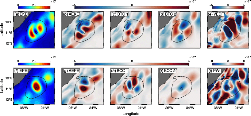
The horizontal structure of the barotropic conversion terms (BTC1 and BTC2 in Fig. 7c, d) exhibits cross- and along-stream positive–negative variability within the eddy area, with elevated positive (negative) values aligned with the eddy core along the zonal (meridional) axis. In the Kuroshio Current, Yan et al. (2022) found similar horizontal patterns and magnitudes between BTC1 and BTC2 terms for a Kuroshio Eddy, with extreme values of ~±0.06 W m−2. Within the average DWBC eddy, we found maximum BTC1 and BTC2 of ~±0.5 W m−2. Apart from the temporal evolution variability of the BTC1 and BTC2 describing the domination of the direct energy cascade at the eddy core depth, the depth-integrated analysis within the average eddy indicated negative values of BTC2 (inverse energy cascade) stronger than positive BTC2 values. Among the 29 isolated eddies, we found maximum BTC1 more than twice as large as BTC2 (4.4 v. 1.8 W m−2 respectively).
Nevertheless, our result highlights the energy conversions within the DWBC eddies, whereas Brum et al. (2023) and Vilela-Silva et al. (2023) analysed the energy conversion in the DWBC mean flow. Brum et al. (2023) computed the 36-year mean barotropic conversion between 5 and 16°S, whereas Vilela-Silva et al. (2023) calculated a 10-year mean horizontal shear production (analogous to the BTC term) between 5 and 15°S. Both studies identified a broad region of mean to eddy barotropic conversion in the centre of the DWBC mean jet, mainly between 9 and 13°S.
By decomposing the BTC1 term (not shown here), we observed that it is largely dominated by the horizontal shear of the alongshore component of the mean flow (∂v̅ ÷ ∂x and ∂v̅ ÷ ∂y). This is expected because the DWBC mean flow has a permanent poleward component, whereas the mean cross-shore component weakens under low-pass filtering.
The along-stream variability in the baroclinic conversion is present in BCC1 and BCC2 (Fig. 7h, i), but the cross-stream variation is only found in BCC1 (Fig. 7h). Near the coast, the mean density gradient intensifies due to increased isopycnal slope, variability in stratification and vertical velocity shear caused by topographic slope, thereby enhancing BCC1 values. Furthermore, BCC1 exhibits values near zero around the eddy centre, whereas BCC2 is elevated. As depicted in Fig. 6, negative BCC2 is in good agreement with areas of negative . In the Kuroshio Current, Yan et al. (2022) found BCC1 and VEDF with extreme values exceeding ±3 × 10⁻² W m−2. Within the average DWBC eddy, we found maximum BCC1 (BCC2) of ~±7 × 10⁻⁴ W m−2 (±3 × 10⁻⁴ W m–2), whereas VEDF reached values over ±2 × 10⁻² W m−2. Among the 29 isolated eddies, we found maximum BCC1 (BCC2) of ~±5 × 10⁻³ W m−2 (±6 × 10⁻⁴ W m–2).
Positive values of AEKE and AEPE are in good agreement with their respective energy reservoir peaks. In this context, the redistribution of EKE by the mean flow (measured by the AEKE term) exhibits a dipole structure in each hemisphere of the eddy, with positive values preceding negative values (Fig. 7b). Depth-integrated EPE (Fig. 7f) shows elevated levels at the eddy centre with maximum values exceeding 6.3 × 10⁴ J m−2, similar magnitude found by Yan et al. (2022) in a Kuroshio Current eddy of ~6.3 × 10⁴ J m−2. The EPE horizontal distribution is aligned with enhanced positive AEPE (Fig. 7g) (indicating the supply of EPE by mean flow advection) and followed by negative values in the Northern Hemisphere. Therefore, the elevated EPE around the eddy core is mainly supplied by mean flow advection rather than baroclinic conversion. Among the 29 isolated eddies, AEKE and AEPE presented maximum values of 4.4 and 2.5 × 10⁻³ W m−2 respectively, which exceeds the maximum values found for the barotropic and baroclinic conversion terms (BTC1, BTC2, BCC1 and BCC2). Therefore, within the DWBC isolated eddies, advection is the main source of EKE and EPE.
Positive VEDF values are found near the eddy boundaries, with elevated levels in the Northern Hemisphere, and negative VEDF is found around the eddy centre (Fig. 7e). Thus, the vertical eddy density fluxes are upgradient (downgradient) to the mean density gradient near the eddy boundaries (around the eddy core), converting EPE → EKE (EKE → EPE). The depth-integrated PW’ exhibits complex spatial structures horizontally inhomogeneous.
Zonal sections at 11°S illustrate the vertical distribution of the energy terms throughout the DWBC layer depth (Fig. 8). Terms related to eddy momentum fluxes are stronger than those related to the eddy density fluxes (elevated only in the upper and lower layers; e.g. Brum et al. 2023). EKE within the average eddy is ~17.0 J m−3 (15.8 J m−3) in the onshore (offshore) lobe, reaching a maximum of 41.7 J m−3 (36.4 J m−3).
Zonal vertical sections at 11°S of eddy energy budgets and eddy–mean flow interaction terms of the averaged DWBC isolated eddy. Solid black lines indicate each eddy lobe boundary. Energy reservoirs (EKE and EPE) are presented in joules per cubic metre, whereas the remaining terms are in watts per cubic metre. Blue and red contour lines in the lower panels indicate elevated perturbation density levels. Grey areas represent the bottom topography. The colour scale is saturated to reveal regions of moderate energy activity.
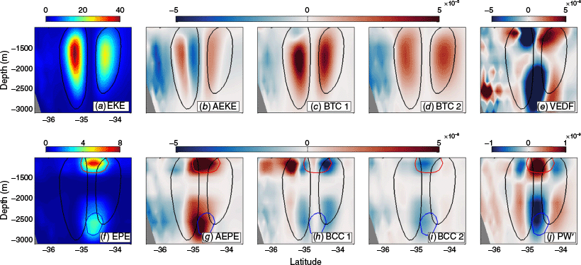
Throughout the depth range of the eddies, barotropic conversion pathway is mainly from the mean flow to the eddy field (direct energy cascade), whereas the baroclinic pathway is dominated by the inverse energy cascade (from the eddy field to the mean flow). Therefore, the available potential energy released by isopycnal slope removes energy from the eddies, supporting the mean flow. Compared to recent studies by Brum et al. (2023) and Vilela-Silva et al. (2023) that also used model output, the barotropic instability pathway towards enhanced EKE is corroborated. However, in the theoretical framework of time-dependent analysis, we find that BTC1 presents a larger conversion rate than BTC2, and that each lobe of the eddy presents a different rate. This result indicates that the mean horizontal shear is responsible for larger barotropic energy conversion than the divergence of eddy momentum fluxes.
The EKE and the two barotropic energy conversion rates (BTC1 and BTC2) exhibit the same structure throughout the depth range of the eddies, with larger values at the eddy core depth and decreasing towards the upper and lower layers. A similar pattern was also observed by Yan et al. (2022) when analysing eddies in the Kuroshio Current.
The vertical distribution of AEKE (Fig. 8b) exhibits positive–negative cross-stream variability within each lobe. A similar pattern is observed in the BCC1 within the onshore lobe, suggesting that near the coast the anticyclones drain energy from the mean DWBC, enhancing the eddy field.
The vertical structure of BCC1 (Fig. 8h) and BCC2 (Fig. 8i) indicates that the interactions between the perturbation density (; Fig. 5f) and the divergence of eddy density fluxes (BCC2) are related to EPE peaks, whereas interactions between eddy density fluxes and the mean density gradient are prominent around the EPE peaks (BCC1). However, despite the good agreement between BCC2 and in Fig. 6 and 7, the positive above the eddy core (Fig. 5f) does not modulate the energy conversion pathway of BCC2 at the same depth. It thus remains unclear to which extent modulates BCC2 throughout the depth range of DWBC eddies at 11°S.
Using model outputs, Lüschow et al. (2019) described the eddy density fluxes decreasing (increasing) potential energy above (below) the core. Moreover, zonally averaged BCC1 and VEDF from Brum et al. (2023) also showed inverse energy conversion pathway between the upper and lower layers of the DWBC in the same region. However, in our analysis, the baroclinic energy conversions related to the EPE (i.e. BCC1, BCC2 and VEDF) presented the same energy conversion pathway throughout the water column within the eddy. Therefore, we conjecture that the zonal means used in previous studies (e.g. Lüschow et al. 2019; Brum et al. 2023) affect the representation of the energy terms distribution within the DWBC eddies, being an aliasing effect on their spatial structure.
The VEDF peaks above and below the eddy (Fig. 8e) (e.g. Brum et al. 2023). This is related to the observed peaks in and not due to stronger eddy activity (elevated eddy activity is found within 1500–2000-m depth, Fig. 8a) (e.g. Lüschow et al. 2019). Moreover, VEDF presented cross-stream positive–negative variability throughout the water column: the vertical eddy density fluxes are downgradient (upgradient) to the mean density gradient around the eddy centre (toward the eddy boundaries), converting EKE → EPE (EPE → EKE).
The EPE, AEPE, BCC2, VEDF and PW′ terms closely correspond to peaks observed in . These terms presented similar horizontal distribution along the water column, with larger values around the eddy centre decreasing towards the boundaries.
The EPE peaks are primarily supplied by mean flow advection, whereas negative BCC2 (VEDF) indicates EPE → MPE (EKE → EPE) conversion. This pattern is consistent with the scenarios observed in Fig. 7.
4.Summary and conclusions
In this contribution, the three-dimensional average structure and temporal evolution of 29 isolated DWBC eddies is discussed. Although eddy–mean flow interaction analyses have been performed in boundary currents under the influence of mesoscale eddies, most studies rely on the eddy-current influence, rather than on the spatiotemporal energy conversions within the mesoscale eddies. As the necessary high-resolution observational data required to perform such analysis is not available, we used 36 years of output from an eddy-resolving (1/10°) OGCM.
Our analysis showed that the DWBC eddies are asymmetric, with the Southern Hemisphere slightly larger than the Northern Hemisphere, and the onshore lobe more energetic than the offshore lobe. Moreover, elevated mean-to-eddy conversion was found towards the coast. Therefore, we suggest that the asymmetry previously observed from velocity records of Dengler et al. (2004) and Schott et al. (2005) is supported by the energy conversion pathway to the eddy field. In addition, Vilela-Silva et al. (2023) suggested that the DWBC eddies near 11°S are influenced by significant eddy–topography interactions, with consequences for mean-to-eddy kinetic energy conversions.
To the best of our knowledge, this is the first temporal description of the eddy–mean flow interaction terms from the EKE and EPE budget equations in an Eulerian frame of reference along the eddy area. The temporal evolution of the EKE budget and related conversion terms exhibited a prominent peak in each hemisphere of the eddy. The average maximum EKE was mainly supported by barotropic conversion driven by the horizontal shear of the mean flow. Conversely, the averaged potential energy budget showed elevated values near the eddy centre, primarily supported by the advection of EPE by the mean flow. Although non-isolated eddies were not included in this study, it is noteworthy that during eddy tracking we observed an abrupt peak in the nonlocal eddy–mean flow interactions term (NLKE term from the MKE budget equation; see eqn A.3 from Brum et al. 2023) during eddy–eddy interaction (not shown here), increasing the magnitude of this term by approximately one to two orders. However, we emphasise that further studies are required to validate this outcome and determine the dynamics related to this interaction.
The average horizontal distribution of the energy terms vertically integrated within the DWBC layer (1000–3000 m) exhibited distinct patterns. Overall, the EKE budget and conversion terms showed elevated values compared to those related to the EPE budget. Within the eddy, the cross- and along-stream positive–negative variability of the barotropic conversion terms exhibited an X-shaped pattern. The EKE was mainly supplied by barotropic conversion and mean flow advection, as measured by BTC1, BTC2 and AEKE terms. However, the EPE budget was mainly supported by mean flow advection (AEPE term). We conjecture that the negative perturbation density within the eddy core (Fig. 5a) was responsible for setting the energy transfer from EPE to MPE due to interaction with the background divergence of eddy density fluxes (indicated by negative BCC2), whereas its elevated variance set the EPE peak associated with the vertical stratification.
Zonal sections at 11°S exhibited stronger EKE in the onshore lobe of the eddy, particularly at the core depth. The potential energy budget and conversion terms were elevated in the upper and lower layers, associated with the perturbation density peak. Apart from the BTC1, BTC2 and BCC2 terms, the remaining terms exhibited intense cross-shore positive–negative variability within each eddy lobe. We conjectured that the areas within the DWBC eddy with elevated positive relative vorticity and large azimuthal velocities induced stronger kinetic energy conversions, whereas elevated perturbation density induced stronger potential energy conversions. In this context, Brum et al. (2023) and Vilela-Silva et al. (2023) found that barotropic instability (MKE → EKE) increases abruptly downstream of the Pernambuco Plateau and contributes to eddy growth.
Regarding the area within the average DWBC isolated eddy, the main conclusions of this work are summarised as follows:
Advection is the main source of EKE and EPE.
Barotropic instability is three orders of magnitude larger than baroclinic instability.
Scaling analysis reveals that vertical pressure work does not significantly influence the energy structure.
Near the coast, the anticyclones drain energy from the mean DWBC enhancing the eddy field.
Above and below the eddy core depth, the three baroclinic energy conversion terms associated with EPE (i.e. BCC1, BCC2 and VEDF) are significantly enhanced, with extreme values occurring near regions of maxima.
Based on the Eulerian framework, the direct energy cascade dominates the barotropic energy conversions during eddy migration, with enhanced conversion rates associated with peaks of eddy velocity. By contrast, the baroclinic energy conversions present alternate energy cascade during eddy migration, and elevated conversion rates are associated with peaks of perturbation density and eddy velocity.
At the eddy core depth, the barotropic (baroclinic) energy pathway contributes to the growth (decay) of EKE (EPE) at a rate of ~1.0 × 10⁻⁶ J m−3 day−1 (5.4 × 10⁻⁶ J m−3 day−1) whereas the eddy migrates at 11°S.
Finally, the continuous eddy generation in this region provides an ideal site for observational programs and numerical modelling investigation of deep eddies energetics and dynamics. Our results provide new insights into the energy budgets and conversion rates within deep mesoscale eddies in western boundary currents and shed light on the mechanisms of time-dependent eddy–mean flow interactions.
Data availability
The OFES model output used in this study is available at https://www.jamstec.go.jp/ofes/ofes.html.
Declaration of funding
This research was undertaken with the assistance of resources and infrastructure from the Ocean and Climate Studies Laboratory, at the Federal University of Rio Grande. A. L. Brum acknowledges the financial support received from Coordenação de Aperfeiçoamento de Pessoal de Nível Superior (CAPES) (grants numbers 88882.158624/2017-07, 88881.189840/2018-01 and 88887.371659/2019-00) and Conselho Nacional de Desenvolvimento Científico e Tecnológico (CNPq) (grants number 382169/2022-0 and 151659/2024-9) funding agencies. J. L. L. de Azevedo thanks the CNPq (grant number 445446/2014-5) and Fundação de Amparo à pesquisa do Estado do Rio Grande do Sul (FAPERGS) (grant number 2325-2551/14-0SIAFEM) funding agencies.
Acknowledgements
We thank the Brazilian CAPES Foundation funding agency for financially supporting the Graduate Program in Oceanology (FURG). The authors thank the anonymous reviewers for their constructive feedback.
References
Adeagbo OS, Du Y, Wang T, Wang M (2022) Eddy–mean flow interactions in the Agulhas leakage region. Journal of Oceanography 78, 151-161.
| Crossref | Google Scholar |
Bower AS, Lozier MS, Gary SF, Böning CW (2009) Interior pathways of the North Atlantic meridional overturning circulation. Nature 459(7244), 243-247.
| Crossref | Google Scholar | PubMed |
Brum AL, Azevedo JLL, Oliveira LR, Calil PHR (2017) Energetics of the Brazil Current in the Rio Grande Cone region. Deep-Sea Research – I. Oceanographic Research Papers 128, 67-81.
| Crossref | Google Scholar |
Brum AL, Azevedo JLL, Dengler M (2023) Energetics of eddy–mean flow interactions in the Deep Western Boundary Current off the northeastern coast of Brazil. Deep-Sea Research – I. Oceanographic Research Papers 193, 103965.
| Crossref | Google Scholar |
Carranza MM, Gille ST, Piola AR, Charo M, Romero I (2017) Wind modulation of upwelling at the shelf-break front off Patagonia: observational evidence. Journal of Geophysical Research: Oceans 122, 2401-2421.
| Crossref | Google Scholar |
Chang Y-L, Miyazawa Y, Guo X (2015) Effects of the STCC eddies on the Kuroshio based on the 20-year JCOPE2 reanalysis results. Progress in Oceanography 135, 64-76.
| Crossref | Google Scholar |
Chen R, Flierl GR, Wunsch C (2014) A description of local and nonlocal eddy-mean flow interaction in a global eddy-permitting state estimate. Journal of Physical Oceanography 44, 2336-2352.
| Crossref | Google Scholar |
Chen X, Qiu B, Chen S, Qi Y, Du Y (2015) Seasonal eddy kinetic energy modulations along the North Equatorial Countercurrent in the western Pacific. Journal of Geophysical Research: Oceans 120, 6351-6362.
| Crossref | Google Scholar |
Chen R, Thompson AF, Flierl GR (2016) Time-dependent eddy–mean energy diagrams and their application to the ocean. Journal of Physical Oceanography 46, 2827-2850.
| Crossref | Google Scholar |
Chern C-S, Wang J (2005) Interactions of mesoscale eddy and western boundary current: a reduced-gravity numerical model study. Journal of Oceanography 61, 271-282.
| Crossref | Google Scholar |
Chiang T-L, Qu T (2013) Subthermocline eddies in the western equatorial Pacific as shown by an eddy-resolving OGCM. Journal of Physical Oceanography 43, 1242-1253.
| Crossref | Google Scholar |
Cronin M, Watts DR (1996) Eddy-mean flow interaction in the Gulf Stream at 68°W. Part I: eddy energetics. Journal of Physical Oceanography 26(10), 2107-2132.
| Crossref | Google Scholar |
de Cuevas BA, Webb DJ, Coward AC, Richmond CS, Rourke E (1999) The UK Ocean Circulation and Advanced Modelling Project (OCCAM). In ‘High-Performance Computing’. (Eds RJ Allan, MF Guest, AD Simpson, DS Henty, DA Nicole) pp. 325–335. (Springer: Boston, MA, USA) 10.1007/978-1-4615-4873-7_35
Dengler M, Schott FA, Eden C, Brandt P, Fischer J, Zantopp RJ (2004) Break-up of the Atlantic Deep Western Boundary Current into eddies at 8°S. Nature 432, 1018-1020.
| Crossref | Google Scholar | PubMed |
Dickey TD, Nencioli F, Kuwahara VS, Leonard C, Black W, Rii YM, Bidigare RR, Zhang Q (2008) Physical and bio-optical observations of oceanic cyclones west of the island of Hawai’i. Deep-Sea Research – II. Topical Studies in Oceanography 10–13, 1195-1217.
| Crossref | Google Scholar |
Dong S, Baringer M, Goni G, Garzoli S (2011) Importance of the assimilation of Argo float measurements on the Meridional Overturning Circulation in the South Atlantic. Geophysical Research Letters 38, L18603.
| Crossref | Google Scholar |
Gary SF, Lozier MS, Böning CW, Biastoch A (2011) Deciphering the pathways for the deep limb of the Meridional Overturning Circulation. Deep-Sea Research – II. Topical Studies in Oceanography 58(17–18), 1781-1797.
| Crossref | Google Scholar |
Garzoli SL, Dong S, Fine R, Meinen CS, Perez RC, Schmid C, van Sebille E, Yao Q (2015) The fate of the Deep Western Boundary Current in the South Atlantic. Deep-Sea Research – I. Oceanographic Research Papers 103, 125-136.
| Crossref | Google Scholar |
Geng W, Xie Q, Chen G, Zu T, Wang D (2016) Numerical study on the eddy–mean flow interaction between a cyclonic eddy and Kuroshio. Journal of Oceanography 72, 727-745.
| Crossref | Google Scholar |
Geng W, Xie Q, Chen G, Liu Q, Wang D (2018) A three-dimensional modeling study on eddy-mean flow interaction between a Gaussian-type anticyclonic eddy and Kuroshio. Journal of Oceanography 74, 23-37.
| Crossref | Google Scholar |
Hummels R, Brandt P, Dengler M, Fischer J, Araújo M, Veleda D, Durgadoo JV (2015) Interannual to decadal changes in the western boundary circulation in the Atlantic at 11°S. Geophysical Research Letters 42, 7615-7622.
| Crossref | Google Scholar |
Jan S, Mensah V, Andres M, Chang M-H, Yang YJ (2017) Eddy-Kuroshio interactions: local and remote effects. Journal of Geophysical Research: Oceans 122, 9744-9764.
| Crossref | Google Scholar |
Jouanno J, Sheinbaum J, Barnier B, Molines JM, Candela J (2012) Seasonal and interannual modulation of the eddy kinetic energy in the Caribbean Sea. Journal of Physical Oceanography 42, 2041-2055.
| Crossref | Google Scholar |
Kang D, Curchitser EN (2015) Energetics of eddy–mean flow interactions in the Gulf Stream region. Journal of Physical Oceanography 45, 103-120.
| Crossref | Google Scholar |
Kang D, Curchitser EN, Rosati A (2016) Seasonal variability of the Gulf Stream kinetic energy. Journal of Physical Oceanography 46, 1189-1207.
| Crossref | Google Scholar |
Krelling APM, Gangopadhyay A, Silveira ICA, Vilela-Silva F (2020) Development of a feature-oriented regional modelling system for the North Brazil Undercurrent region (1°S–11°S) and its application to a process study on the genesis of the Potiguar Eddy. Journal of Operational Oceanography 15(2), 69-86.
| Crossref | Google Scholar |
Lee TN, Johns WE, Zantopp RJ, Fillenbaum ER (1996) Moored observations of Western Boundary Current Variability and thermohaline circulation at 26.5° in the Subtropical North Atlantic. Journal of Physical Oceanography 26(6), 962-983.
| Crossref | Google Scholar |
Liu J, Zheng S, Feng M, Xie L, Feng B, Liang P, Wang L, Yang L, Yan L (2022) Seasonal variability of eddy kinetic energy in the East Australian Current region. Frontiers in Marine Science 9, 1069184.
| Crossref | Google Scholar |
Lumpkin R, Speer K (2007) Global Ocean Meridional Overturning. Journal of Physical Oceanography 37, 2550-2562.
| Crossref | Google Scholar |
Lüschow V, Von Storch J-S, Marotzke J (2019) Diagnosing the influence of mesoscale eddy fluxes on the Deep Western Boundary Current in the 1/10° STORM/NCEP simulation. Journal of Physical Oceanography 49, 751-764.
| Crossref | Google Scholar |
Magalhães FC, Azevedo JLL, Oliveira LR (2017) Energetics of eddy-mean flow interactions in the Brazil Current between 20°S and 36°S. Journal of Geophysical Research: Oceans 122, 6129-6146.
| Crossref | Google Scholar |
Masumoto Y (2010) Sharing the results of a high-resolution ocean general circulation model under a multi-discipline framework – a review of OFES activities. Ocean Dynamics 60, 633-652.
| Crossref | Google Scholar |
Napolitano DC, Silveira ICA, Rocha CB, Flierl GR, Calil PHR, Martins RP (2019) On the steadiness and instability of the Intermediate Western Boundary Current between 24 and 18°S. Journal of Physical Oceanography 49, 3127-3143.
| Crossref | Google Scholar |
Nencioli F, Dong C, Dickey T, Washburn L, McWilliams JC (2010) A vector geometry-based eddy detection algorithm and its application to a high-resolution numerical model product and high-frequency radar surface velocities in the Southern California Bight. Journal of Atmospheric and Oceanic Technology 27, 564-579.
| Crossref | Google Scholar |
Olson DB (1991) Rings in the ocean. Annual Reviews of Earth Planetary Science 19, 283-311.
| Crossref | Google Scholar |
Perez RC, Garzoli SL, Meinen CS, Matano RP (2011) Geostrophic velocity measurement techniques for the Meridional Overturning Circulation and meridional heat transport in the South Atlantic. Journal of Atmospheric and Oceanic Technology 28, 1504-1521.
| Crossref | Google Scholar |
Qiu B, Chen S, Klein P, Sasaki H, Sasai Y (2014) Seasonal mesoscale and submesoscale eddy variability along the North Pacific subtropical Countercurrent. Journal of Physical Oceanography 44, 3079-3097.
| Crossref | Google Scholar |
Rhein M, Stramma L (2005) Seasonal variability in the Deep Western Boundary Current around the eastern tip of Brazil. Deep-Sea Research – I. Oceanographic Research Papers 52, 1414-1428.
| Crossref | Google Scholar |
Rhein M, Stramma L, Send U (1995) The Atlantic Deep Western Boundary Current: water masses and transports near the equator. Journal of Geophysical Research 100, 2441-2457.
| Crossref | Google Scholar |
Rieck JK, Böning CW, Greatbatch RJ, Scheinert M (2015) Seasonal variability of eddy kinetic energy in a global high-resolution ocean model. Geophysical Research Letters 42, 9379-9386.
| Crossref | Google Scholar |
Schott FA, Fischer J, Reppin J, Send U (1993) On mean and seasonal currents and transports at the western boundary of the Equatorial Atlantic. Journal of Geophysical Research 98(C8), 14353-14368.
| Crossref | Google Scholar |
Schott FA, Dengler M, Brandt P, Affler K, Fischer J, Bourlès B, Gouriou Y, Molinari RL, Rhein M (2003) The zonal currents and transports at 35°W in the tropical Atlantic. Geophysical Research Letters 30(7), 1349.
| Crossref | Google Scholar |
Schott FA, Dengler M, Zantopp RJ, Stramma L, Fischer J, Brandt P (2005) The shallow and deep western boundary circulation of the South Atlantic at 5–11°S. Journal of Physical Oceanography 35, 2031-2053.
| Crossref | Google Scholar |
Schulzki T, Getzlaff K, Biastoch A (2021) On the variability of the DWBC transport between 26.5°N and 16°N in an eddy-rich ocean model. Journal of Geophysical Research: Oceans 126, e2021JC017372.
| Crossref | Google Scholar |
Solodoch A, McWilliams JC, Stewart AL, Gula J, Renault L (2020) Why does the Deep Western Boundary Current “leak” around Flemish Cap? Journal of Physical Oceanography 50(7), 1989-2016.
| Crossref | Google Scholar |
van Sebille E, Johns WE, Beal LM (2012) Does the vorticity flux from Agulhas rings control the zonal pathway of NADW across the South Atlantic? Journal of Geophysical Research 117, C05037.
| Crossref | Google Scholar |
Vilela-Silva F, Silveira ICA, Napolitano DC, Souza-Neto PWM, Biló TC, Gangopadhyay A (2023) On the Deep Western Boundary Current separation and anticyclone genesis off northeast Brazil. Journal of Geophysical Research: Oceans 128(1), e2022JC019168.
| Crossref | Google Scholar |
Vilela-Silva F, Bindoff NL, Phillips HE, Rintoul SR, Nikurashin M (2024) The impact of an Antarctic Circumpolar Current meander on air–sea interaction and water subduction. Journal of Geophysical Research: Oceans 129(7), e2023JC020701.
| Crossref | Google Scholar |
Von Storch J-S, Eden C, Fast I, Haak H, Deckers DH, Reimer EM, Marotzke J, Stammer D (2012) An estimate of the Lorenz energy cycle for the world ocean based on the 1/10° STORM/NCEP simulation. Journal of Physical Oceanography 42, 2185-2205.
| Crossref | Google Scholar |
Wang Q (2017) Three-dimensional structure of mesoscale eddies in the western tropical Pacific as revealed by a high-resolution ocean simulation. Science China Earth Sciences 60, 1719-1731.
| Crossref | Google Scholar |
Yamagami Y, Tozuka T, Qiu B (2019) Interannual variability of the Natal Pulse. Journal of Geophysical Research 124, 9258-9276.
| Crossref | Google Scholar |
Yan X, Kang D, Curchitser EN (2019) Energetics of eddy-mean flow interactions along the western boundary currents in the North Pacific. Journal of Physical Oceanography 49, 789-810.
| Crossref | Google Scholar |
Yan X, Kang D, Pang C, Zhang L, Liu H (2022) Energetics analysis of the Eddy–Kuroshio interaction east of Taiwan. Journal of Physical Oceanography 52, 647-664.
| Crossref | Google Scholar |
Yan X, Kang D, Curchitser EN, Liu X, Pang C, Zhang L (2023) Seasonal variability of eddy kinetic energy along the Kuroshio Current. Journal of Physical Oceanography 53, 1731-1752.
| Crossref | Google Scholar |
Yang Y, Liang XS (2016) The instabilities and multiscale energetics underlying the mean-interannual–eddy interactions in the Kuroshio Extension Region. Journal of Physical Oceanography 46, 1477-1494.
| Crossref | Google Scholar |
Yang G, Wang F, Li Y, Lin P (2013) Mesoscale eddies in the northwestern subtropical Pacific Ocean: statistical characteristics and three-dimensional structures. Journal of Geophysical Research: Oceans 118(4), 1906-1925.
| Crossref | Google Scholar |
Yang C, Chen X, Cheng X, Qiu B (2020) Annual versus semi-annual eddy kinetic energy variability in the Celebs Sea. Journal of Oceanography 76, 401-418.
| Crossref | Google Scholar |
Zhang N, Liu G, Liu Q, Zheng S, Perrie W (2020) Spatiotemporal variations of mesoscale eddies in the southeast Indian Ocean. Journal of Geophysical Research: Oceans 125(8), e2019JC015712.
| Crossref | Google Scholar |
Zhang L, Hui Y, Qu T, Hu D (2021) Seasonal variability of Subthermocline eddy kinetic energy east of the Philippines. Journal of Physical Oceanography 51, 685-699.
| Crossref | Google Scholar |
Zhang L, Song W, Hui Y, Wang Z, Hu D (2024) Subsurface eddies east of the Philippines: geographic characteristics, vertical structures, volume, and thermohaline transport. Progress in Oceanography 222, 103228.
| Crossref | Google Scholar |