

Automated methods for processing camera trap video data for distance sampling
Trevor Bak A * , Richard J. Camp B , Matthew D. Burt C and Scott Vogt D
A
B
C
D
Abstract
Population monitoring is an essential need for tracking biodiversity and judging efficacy of conservation management actions, both globally and in the Pacific. However, population monitoring efforts are often temporally inconsistent and limited to small scales. Motion-activated cameras (‘camera traps’) offer a way to cost-effectively monitor populations, but they also generate large amounts of data that are time intensive to process.
To develop an automated pipeline for processing videos of ungulates (Philippine deer, Rusa marianna; and pigs, Sus scrofa) on Andersen Air Force Base in Guam.
We processed camera videos with a machine learning model for object detection and classification. To estimate density using distance sampling methods, we used a separate machine learning model to estimate the distance of target animals from the camera. We compared density estimates generated using manual versus automated methods and assessed accuracy and processing time saved.
The object detection and classification model achieved an overall accuracy >80% and F1 score ≥0.9 and saved 36.9 h of processing time. The automated distance estimation was fairly accurate, with a 1.1 m (±1.4 m) difference from manual distance estimates, and saved 16.8 h of processing time. Density estimates did not differ substantially between manual and automated distance estimation.
Machine learning models accurately processed camera videos, allowing efficient estimates of density from camera data.
Further adoption of motion-activated cameras coupled with automated processing could lead to continuous, large-scale monitoring of populations, helping to understand and address changes in biodiversity.
Keywords: automated processing, biodiversity, camera traps, conservation management, distance sampling, Guam, machine learning, ungulates.
Introduction
Population monitoring and biodiversity
Population monitoring is fundamental to understanding biodiversity trends, addressing the accelerated rate of modern biodiversity loss, and directing limited conservation resources to species and ecosystems in greatest need (Ceballos et al. 2017; Diaz et al. 2019; Jetz et al. 2019). Assessing the efficacy of international agreements to halt biodiversity decline, such as the Kunming-Montreal Global Biodiversity Framework, requires population monitoring (Convention on Biological Diversity 2022). Corresponding frameworks for preserving Pacific biodiversity, such as the Pacific Islands Framework for Nature Conservation and Protected Areas 2021–2025, also utilise population monitoring as a primary means of assessing progress towards biodiversity goals (SPREP 2021). Biodiversity preservation is especially needed in the Pacific region given high levels of island biodiversity coupled with pronounced species declines and extinctions (Jupiter et al. 2014).
However, population monitoring efforts are often spatially limited and conducted in a temporally inconsistent manner (Bayraktarov et al. 2019). At least a decade of continuous monitoring is typically needed to assess population trends and to separate meaningful changes in population from natural oscillations (White 2019), but monitoring schemes typically occur over shorter intervals due to funding constraints (Hughes et al. 2017). These inconsistencies make detecting ecosystem trends and understanding the effects of conservation actions difficult. Furthermore, once a time series is interrupted, re-establishing monitoring can be difficult and expensive (Bayraktarov et al. 2019). Approaches to population monitoring that are more continuous and scalable could help address biodiversity preservation goals.
Motion-activated cameras
Conventional population monitoring techniques rely on humans collecting field data, but sending humans into the field is a costly and resource intensive endeavour (Witmer 2005). Cost issues are especially acute in the tropics, which tend to receive less funding compared to more developed regions (Balmford and Whitten 2003; Moussy et al. 2022) and where the remoteness and ruggedness of the terrain may increase field costs due to field sites being difficult to access and traverse. The most common population monitoring methods are based on capture–recapture and related methods that require marking or uniquely identifying individuals to create individual encounter history data (Amstrup et al. 2005). Capturing, marking, and either recapturing or resighting individuals repeatedly requires substantial time, field crew, and financial costs (Field et al. 2005). Other population monitoring schemes, such as distance sampling, which involves observers recording detections and distances of a species of interest, can also be resource intensive (Anderson et al. 2013; Keeping et al. 2018). These costs contribute to inconsistent sampling efforts and infrequent population monitoring (Bayraktarov et al. 2019).
Motion-activated cameras (also referred to as ‘camera traps’) offer a solution to this problem, providing a continuous, scalable, and potentially low-cost way to monitor animals in the field. Although motion-activated cameras require higher upfront capital costs and thus can be more expensive than traditional methods for short sampling time frames, lower logistical and staff costs lead to cost savings over longer sampling time frames (Lyra-Jorge et al. 2008; De Bondi et al. 2010; Welbourne et al. 2015). Logistical costs are minimised over time as field teams only need to go to the field to setup and retrieve the cameras, and to perform maintenance such as replacing batteries and storage cards (Cappelle et al. 2019). Cameras can also be reused between projects, yielding lower overall costs for research teams consistently engaged in population monitoring. Given their efficacy and cost effectiveness, motion-activated cameras have been used across a range of environments and species and the use of motion-activated cameras has been growing strongly since the mid-2000s, when the technology started to become more widely adopted (Rovero and Zimmermann 2016; Delisle et al. 2021). Motion-activated cameras have been used in the Pacific to assess levels of activity of invasive rats on Phillip Island in Australia (Rendall et al. 2014), the spatial distribution and impact of hunting management action on ungulates across Hawaiian Islands (Judge et al. 2016; Risch et al. 2025), and yǻyaguak (Aerodramus bartschi; Mariana Swiftlet) population densities on Saipan Island, where manual detection ability is limited (Gorresen et al. 2024).
Camera trap distance sampling (CTDS; Howe et al. 2017) combines distance sampling, which accounts for imperfect detection, with camera data. This allows for continuous sampling that produces reliable density estimates of unmarked animals. CTDS also enables widespread spatial coverage and has been successfully used across a variety of taxa and regions while maintaining high precision (i.e. low coefficient of variation in density estimates; Cappelle et al. 2021; Mason et al. 2022). However, accurate CTDS density estimates require certain assumptions to be met: that cameras are distributed independent of animal locations with a random design component, that all animals at zero distance are detected, and that animals move in and out of the field of view at random (Howe et al. 2017). Additionally, the target species must be active and available for detection, which is accounted for in CTDS by analysing temporal activity by time of day and incorporating the proportion of time animals are active as a parameter in the distance sampling model (Rowcliffe et al. 2014; Howe et al. 2017).
Automated methods
Despite the advantages of motion-activated cameras, they have their drawbacks, specifically the immense amounts of data that need to be processed, necessitating substantial human effort and costs (Norouzzadeh et al. 2018). To address the large amounts of data generated by cameras, automated methods for processing camera data have been developed (Tabak et al. 2019). Numerous studies have recently been published utilising machine learning models with camera data for object detection (is a species present?) and identification (if present, what is the species?) with most studies finding high levels of accuracy and large decreases in processing times (Choiński et al. 2021; Fennell et al. 2022; Tan et al. 2022). A range of object detection and classification models have been used with some of the most common being Megadetector for object detection (Beery et al. 2019), and Machine Learning for Wildlife Image Classification, Conservation AI, and Wildlife Insights for object detection and classification (Vélez et al. 2023). All these models are based on deep neural networks that mimic, to some degree, the way the human brain works and can apply information learned from training data to novel datasets (i.e. novel species and environments; Fennell et al. 2022). Automated classification of camera data can lead to substantial reductions in manual labour required, with a greater than 99% reduction in processing time for very large datasets (e.g. datasets with millions of images), while performing at the same or higher levels of accuracy as humans (Norouzzadeh et al. 2018).
To facilitate CTDS sampling population estimation, which requires a distance estimate for each species detection, methods to automatically estimate the distance of a target species from the camera have also been developed (Haucke et al. 2022; Johanns et al. 2022). These methods build on earlier pioneering work that explored how to turn two dimensional images into three dimensional models (Hoiem et al. 2005; Saxena et al. 2009). This projection of two dimensional space into three dimensional space allows for estimation of where objects occur in the image along the third axis or the depth dimension. Depth estimations have been applied to a range of images (Facil et al. 2019) and more recently have been applied to camera imagery to enable distance sampling analyses (Haucke et al. 2022; Johanns et al. 2022). A recent advancement in depth estimation for distance sampling from camera data allows for estimating the depth of animals without the need for model calibration based on reference landmarks (Johanns et al. 2022). This advancement builds on work by Yin et al. (2021) and uses a scaling metric to convert relative depth to absolute depth, which is then used for animal distance estimation.
Study aims
In this study, we developed an automated pipeline for processing videos of ungulates (Philippine deer, Rusa marianna; and pigs, Sus scrofa) on Andersen Air Force Base in Guam. Control of ungulates is a basic conservation management need, as ungulates can cause serious damage to native ecosystems on Pacific Islands (Gawel et al. 2018). In Guam, for example, introduced deer browse on native plants while impeding seed dispersal (Gawel et al. 2018). Consequently, removal of ungulates on Pacific Islands can help restore native plant communities and improve ecosystems (Hess et al. 2010; Litton et al. 2018). To address the negative effects of ungulates on Guam, hunting management actions were carried out in the study area prior to camera deployment and Andersen Air Force Base requested estimates of ungulate density to help assess the efficacy of management actions.
Our specific aims in this study are to: (1) implement two machine learning models for object detection and identification; (2) implement a machine learning model for estimating distance of animal to camera; (3) compare object detection and identification accuracy between the two machine learning models and assess machine learning distance estimation accuracy; (4) compare density estimates between manual and automated distance estimates; and (5) assess the amount of classification and distance estimation processing time saved by using automated methods.
Methods
Camera videos
We deployed 39 motion-activated cameras at 39 sites on Andersen Air Force Base on the island of Guam from 20 January to 9 May 2022, for the purpose of monitoring ungulates with video recording. Cameras were installed in jungle understorey in a 500 m × 500 m regular grid with a random start point. Cameras were outward-facing and secured to trees at a height of 30–50 cm with an orientation parallel to the ground slope. Cameras were deployed in flat terrain. The cameras used were Moultrie A-Series Digital Game Cameras (Model MCG-13296; PRADCO Outdoor Brands, Calera, Alabama, USA) and Bushnell Trophy Cameras (Model 119876; Bushnell Outdoor Products, Overland Park, Kansas, USA). The cameras operated continuously and recorded video when motion was detected by passive infra-red sensors. The cameras had a default 15 s video recording length and were programmed to use the fastest trigger times (0.2 s for Bushnell and 0.7 s for Moultrie cameras). Cameras were first deployed with a north orientation and then rotated to face south to sample microsite conditions. More details of camera deployment are provided in Camp et al. (2025).
Automated object identification and classification
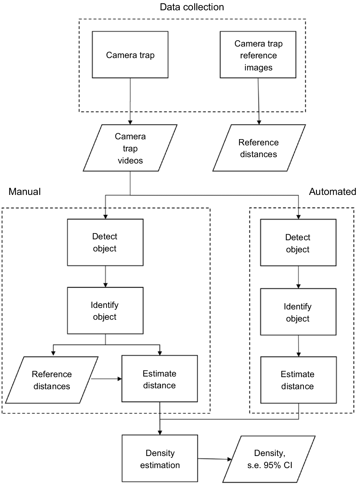
We used a combination of machine learning models to assess our camera data and generate distance estimates (Fig. 1). To automatically classify videos, we used the open-source video processing machine learning software Zamba Cloud ver. 2.1.0, developed by DrivenData (DrivenData Inc, Denver, Colorado; https://zamba.drivendata.org/). We tested two Zamba models: the African model, which was trained on 250,000 videos collected in Africa, and the European model, which further refined the African model by training on an additional ~13,000 videos from motion-activated cameras in Germany. We decided to test two different models as they each had unique advantages and disadvantages. The European model featured species (European roe, Capreolus capreolus; and wild boar) that were similar to our target species of interest, Philippine deer and pig. The European roe is a relatively small deer about 95–135 cm long and 63–67 cm at the shoulder (Macdonald and Barrett 1993). Tropical island pigs are generally smaller than European wild boars due to hybridisation between the east Asiatic lineage, brought by Polynesians, and European domestic pigs, but overall they are similar in morphology (Tomich 1986; Linderholm et al. 2016). However, the temperate European background differed more from our tropical background. In contrast, the African model featured animals (duikar, (identified to the subfamily; Cephalophinae) and hog (made up of a variety of pigs from the Potamochoerus genus along with Hylochoerus meinertzhageni)) less similar to our target species but with a tropical background more similar to our background. Two research team members manually classified a subset of videos in order to assess the accuracy of the Zamba model.
Data processing pipeline for classifying motion-activated cameras videos and estimating distance of target species from camera. Boxes represent a process and trapezoids represent an output, with arrows showing depicting how data moves from one step to the next. Processing pipelines are split between manual and automated (machine learning based) methods. Results from both pipelines are then used for estimating densities using distance sampling methods.
Automated distance estimation
To account for potential differences in detections by camera types, we ran distance sampling models for deer and pig with camera type as a covariate and compared the model fit and detection probability (see Supplementary material file S1 and Fig. S1). For automated estimation of the distance between the camera and observed animal we used the code described in Johanns et al. (2022; available on GitHub at https://github.com/PJ-cs/DistanceEstimationTracking). For videos that contained the target species we split the video into images at predetermined intervals, called snapshot moments (i.e. at intervals of 1, 3, 5, 7, 9, 11, 13, and 15 s in the video). Images without the target species were discarded (e.g. snapshot moments where the target species had left the frame after 3 s). The snapshot images were then processed by the automated distance estimation model that first used Megadector (Beery et al. 2019) to identify animals and draw a bounding box around each animal, and then processed with a DINO model (self-DIstillation with NO labels; Caron et al. 2021) to create a segmentation mask. A segmentation mask identifies each pixel that makes up part of the animal, such that DINO more accurately identifies the animal within the bounding box (Johanns et al. 2022). Distance estimation for each animal was estimated using the median pixel depth of the respective segmentation mask.
Distance was manually estimated for a subset of images by two research team members to assess accuracy of the automated distance estimation model and allow for comparison of population density estimates between manual and automated distance estimates. To estimate distance, we compared the location of target individuals to reference distances of artificial (surveys flags from 1 m to 15 m) and natural (flagged trees and branches) marks at known distances from the camera. For individuals detected along the sides of the field of view, we compared animal locations to reference videos taken for each camera installation where a research team member held signs noting distances and traversed across the field of view at those distances.
Accuracy statistics
We used a subset of receiver operating characteristic analyses to assess Zamba model performance, as is common in assessments of machine learning accuracy (e.g. Fennell et al. 2022; Tan et al. 2022). For each video Zamba classified, we received three labels with confidence values, with the first label being the highest confidence one. We used only the first label and did not use a threshold for confidence values (a practice wherein labels below a confidence threshold are not used) in order to evaluate accuracy statistics for all videos and maximise the number of videos passed on to the next step. We used an R (R Core Team 2022) script to combine manual and Zamba labels into one dataset and assess accuracy between the two approaches. For instances where manual and Zamba labelling disagreed we performed a second round of manual classification that we considered the ‘true’ label. This accounted for instances where the Zamba label was correct, and the human label was incorrect, such as videos featuring a deer at night far from the camera with the silhouette barely visible. For our purposes, we defined a true positive as being when both automated and manual methods assigned a video as having a target species, and a true negative as being when both methods classified a video as blank (no objects in the video) or having a non-target species. We defined a false positive as a video identified by Zamba as featuring a target species when the target species was not present, and a false negative as a video identified by Zamba as not having a target species present, when one was present. This permitted computing misclassification. The following accuracy statistics were calculated:
Overall accuracy:
Precision:
Recall:
F1 score:
Overall accuracy represents the percentage of correct labels assigned. The precision score represents the rate of false positives to true positives and the recall score represents the rate of false negatives to true positives. The F1 score represents the balance of false positives to false negatives and ranges from 0 to 1. We also generated confusion matrices for each model and species to show counts for true negative, false positive, false negative, and true positive. We calculated overall accuracy for a subset of videos with labels with a confidence <0.5, to assess if our approach of not using a threshold value meant large amounts of inaccurate videos were being retained, or if low confidence labels were still accurate enough to be useful. To assess the accuracy of the distance estimation model we determined the difference between manual estimates of distance when the target species was standing next to a reference flag and automated estimates of distance for the same image. We computed the mean and standard deviation of the differences.
Differences in density estimates
To assess differences in density estimation by distance estimator (manual vs automated), we ran independent distance sampling models for each distance estimator and species (for a total of four models). We used a subset of data where both manual and automated processes estimated the distance for the same image, so that comparison was done with the same underlying data. A hazard rate detection function model was used for deer based on hazard rate having the lowest Akaike information criterion. For pig, the hazard rate failed to converge for manual distance estimates, so we used the more parsimonious half normal detection function model for both estimators to allow for comparison. We accounted for temporal availability by using R package activity (Rowcliffe 2019) and accounted for temporal activity following methods described in Howe et al. (2017). We then ran a thousand bootstrap iterations and computed median density estimates, along with calculating s.e., confidence intervals, and coefficient of variation (CV; calculated as ). Density estimates based on all data collected are described in Camp et al. (2025). We also ran distance estimator as a covariate in a single hazard rate model for deer and half normal model for pig to assess how detection function fit varied by distance estimator.
Time saved
To estimate the amount of manual classification processing time saved by using Zamba for video classification, we first recorded how long it took a researcher to manually classify 50 videos and computed the average time it took to classify one video, defined as Tpv. From this we calculated how much time was saved with automated classification using the equation:
where Ts is time saved, Nz is number of videos Zamba classified, and Nhv is number of videos manually classified.
Similarly, to estimate the amount of manual distance estimation processing time saved, we recorded the time it took a researcher to manually estimate and record distance for 50 snapshot images, and then computed the average time it took to classify one video, defined as Tps. We then calculated the number of time saved as:
where Ts is time saved, Na is the number of snapshot images distance was estimated using the automated distance model, and Nhs is the number of snapshot images where observation distances were manually estimated. Time was recorded in seconds for both equations. We did not account for processing time it took to use the automated methods and check accuracy as this was an exploratory analysis and processing time will be highly variable by research team and experience.
Results
Data processing
We collected a total of 7695 videos, and we manually assessed 1628 videos for object detection and identification to assess Zamba accuracy. We processed all of our videos with Zamba, and Zamba identified 638 videos contained deer, 836 contained pig, and 4572 were blank. An additional 1649 videos contained ‘other’ objects (humans, vehicles, non-target species). From the 1474 videos that contained a target species, we created 7189 snapshot images. Slightly more than 64% (4631) of the snapshot moments were successfully processed by the automated distance estimation model, and associated distance estimates were generated. Distances were estimated for 2031 deer and 2101 pigs using automated methods. The distance estimation model failed to process 2558 images; for these images two members of the research team manually estimated the distances.
Accuracy statistics
Accuracy statistics showed the European model had higher accuracy for identifying our target species (Table 1) than the African model (Table 2); however, the African model had higher accuracy at identifying blank videos (Table S1). For the European model, accuracy was >80% for deer and pigs on both orientations, while precision and recall were >90%. The F1 score was above 0.9 for both orientations and both target species and all objects. The African model had lower accuracy of between 39.3% and 67.4% across orientations and objects. However, in general precision was higher than the European model, with precision >94% and even 100% for some objects and orientations, with a correspondingly small number of false positives. Given the higher accuracy of the European model, we used this model for identifying videos with target species for the next steps in the automation pipeline.
| Statistic | North orientation | South orientation | |||||
|---|---|---|---|---|---|---|---|
| Deer | Pig | All objects | Deer | Pig | All objects | ||
| Accuracy | 83.1% | 84.2% | 82.7% | 81.6% | 80.5% | 78.2% | |
| Precision | 95.8% | 93.2% | 92.7% | 92.1% | 92.1% | 94.4% | |
| Recall | 94.8% | 96.1% | 94.2% | 91.0% | 87.7% | 90.1% | |
| F1 | 0.95 | 0.95 | 0.93 | 0.92 | 0.90 | 0.92 | |
Statistics are presented by camera orientation and for deer, pigs, and all objects. The number of videos in each category are provided.
| Statistic | North orientation | South orientation | |||||
|---|---|---|---|---|---|---|---|
| Deer | Pig | All objects | Deer | Pig | All objects | ||
| Accuracy | 57.4% | 49.2% | 48% | 67.4% | 39.3% | 41.5% | |
| Precision | 94.2% | 100% | 94.3% | 100% | 97.8% | 98.6% | |
| Recall | 84.4% | 78.0% | 73.2% | 78% | 50% | 58.6% | |
| F1 | 0.89 | 0.88 | 0.82 | 0.88 | 0.66 | 0.74 | |
Statistics are presented by camera orientation and for deer, pigs, and all objects. The number of videos in each category are provided.
To assess the effect of not using a threshold confidence for labels, we assessed the overall accuracy of low confidence (probability ≤0.5) classification. Low confidence classifications were uncommon, making up only 10.2% of labels, and overall accuracy for these low confidence labels was 39.3%. Low probability labels were largely blank videos (Supplementary file S2, Table S2), and incorrect low probability labels were blank false positive videos (Table S3). Differences in the distance estimates between manually and automated methods for animals observed next to a reference flag was on average 1.07 m (s.d. 1.44 m). The automated procedure, in general, tended to place animals further from the camera than manually estimated distances.
Differences in density estimation
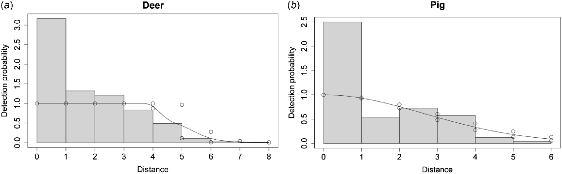
Distances were estimated by manual and automated methods for the same set of images for 131 pig and 422 deer snapshot moments. For deer, we found no difference in median density estimation between manual and automated distance estimates, although the s.e. and consequently CV for manual estimates were higher (Table 3). When distance estimator was run as a covariate in a hazard rate detection function model, differences in detection probabilities were very minor except for at distance bin of 5 m, where divergence was larger (Fig. 2). For pig, manual distance estimates had a higher median density estimation (~1.4 × higher) and again manual distance estimates had higher s.e. and a very large CV (Table 3). When distance estimator was run as a covariate in a half normal model, the detection probabilities between manual and automated methods were very similar (Fig. 2).
| Median | s.e. | LCL | UCL | CV | ||
|---|---|---|---|---|---|---|
| Pig | ||||||
| Automated | 0.19 | 0.08 | 0.05 | 0.36 | 0.42 | |
| Manual | 0.26 | 0.99 | 0.05 | 0.69 | 3.81 | |
| Deer | ||||||
| Automated | 0.33 | 0.16 | 0.14 | 0.77 | 0.48 | |
| Manual | 0.33 | 0.39 | 0.1 | 1.47 | 1.19 | |
Median is the median density estimate of the 1000 bootstrap iterations; LCL, lower confidence limit; UCL, upper confidence limit; CV, coefficient of variation.
Detection probability plot with histogram of distances for human or automated estimator as covariate for (a) Philippine deer (Rusa marianna) with hazard rate detection function model and (b) pig (Sus scrofa) with half normal detection function model. Detection probabilities are similar, except for deer at 5 m, indicating manual and automated distance estimates lead to similar detection probabilities.
Processing time saved
We found that utilising automated methods led to a large reduction in processing time for classifying videos and estimating distances. A member of the research team took 20 min and 44 s to classify 50 videos, for a per video processing time of 24.9 s. This led to 36.8 h of processing time saved by using Zamba. Similarly, a member of the research team took 13 min to estimate and record the distance for 50 snapshot images, for a per video processing time of 15.6 s. This led to 16.5 h of processing time saved.
Discussion
Overall, automated methods worked well to classify videos and generate distance estimates for a large portion of our data. Zamba accuracy was fairly high and automated distance estimation lead to similar density estimates as compared to manual distance estimates. Processing time saved was notable and future research teams using larger datasets would see very large reductions in processing times. Overall, our pipeline provides an effective and time saving way to generate density estimates from unmarked animals and shows classification models trained in temperate environments can work well in tropical island environments.
Automated object identification and classification
We found the Zamba European model ver. 2.1.0 accurately classified species in our dataset (Table 1). Machine learning models tend to generalise poorly to novel datasets, such as species and backgrounds that are different from the data the model has been trained on, hindering wider spread use of automated classification (Beery et al. 2018; Whytock et al. 2021). In this context, the performance of the European model on accurately classifying novel species in a novel background is particularly noteworthy. Our accuracy results are in line with, and only slightly lower, than recent use cases of automated classification models (e.g. Megadetector, Cascade R-CNN, FCOS), which found accuracy, precision, and recall above 90%, and F1 scores above 0.8 (Choiński et al. 2021; Fennell et al. 2022; Tan et al. 2022). Our target species were morphologically similar to the species in the European model, which likely contributed to the high model accuracy. Supporting this, the African model detected blank images well, as represented by the high precision values, which indicates very low false positives, but had lower overall accuracy (Table 2). Thus, the African model did a better job distinguishing objects from the background but performed worse for our study purpose of identifying deer and pigs. Studies with target species different from the species the machine learning model was trained on would likely benefit from additional training on animals specific to their dataset. It appears background consistency between the training data and study data is less important for identifying species of interest, although lack of background similarity could lead to higher false positive rates.
The target species in our study were large-bodied mammals that readily triggered the cameras and took up a sizable portion of the video. Detecting smaller bodied species is possible; for example, the DrivenData African model identifies species as small as mongoose and rodent. However, there is a point at which an object becomes too small to reliably detect and classify. Humans are still able to much more reliably detect very distant animals (e.g. animals that appear as small objects), with humans having a minimum detection size limit 15 times greater than Megadetector (Leorna and Brinkman 2022). Because motion activated cameras themselves need to detect movement to trigger, the limitation in detecting small species could be the camera rather than the machine learning classifier. One study found the minimum detection size for Megadetector was ~10 times smaller than the minimum detection size for the motion activated camera used (Reconyx HyperFire 2 HF2X; Leorna and Brinkman 2022).
In practice, the setup of the camera and the target species determines the feasibility of detecting small species; the key element is how big the species is in the camera image. For example, mosquitos have been successfully identified with machine learning classifiers but this is based on a trap setup where the camera is placed to take ‘close up’ images of mosquitos once they are in the trap (Liu et al. 2023). In contrast, detecting insects or other very small animals with our camera setup would not be possible. In addition to body size, morphological similarity between the species of interest is also a concern. Our target species, deer and pig are rather distinct morphologically. However, for morphologically similar species, machine learning is less accurate at classifying to the species level and may not perform well enough for conservation manager needs (Diggins et al. 2022). For detecting small species in the environment with automated approaches, another possibility is passive acoustic monitoring (Sugai et al. 2019). For bird species with small bodies visual classification may not be possible, but machine learning can classify bird species based on their presence in the soundscape. Bird calls can be tracked with a spectrogram, and the spectrogram image can be classified with machine learning to identify species by their calls (Silva et al. 2022). Although density estimation is harder with passive acoustic monitoring, new techniques to estimate density are being developed (Pérez-Granados and Traba 2021; Navine et al. 2024; Brueggemann et al. 2025). Depending on the management needs, conservation managers could adopt several of these approaches to monitor wildlife with automated methods.
Automated distance estimation
Using automated distance estimation methods helped estimate distances for a large number of animals but the high processing failure rate (36%) required manually estimating distances for more than 2000 snapshot moment images. Reasons for failures included batches failing to process, distance estimates not being generated for all images uploaded (e.g. 400 images were uploaded but distance estimates only came back for 300), and negative distance estimates being generated. Some of the issues may have been due to how we processed the images. We uploaded our images to a cloud-based coding environment rather than running the script locally (running locally is likely to be more stable and have fewer processing failures). We also found some degree of inaccuracy in automated estimates of distance, with a mean error of 1.07 m (s.d. 1.44 m). However, humans are also inaccurate in estimating distance from camera data. In one study, five participants had a s.e. of 0.62 m showing variability in human distance estimates (Haucke et al. 2022). Further, inaccuracies in distance estimation did not appear to unduly bias our density estimates.
Density estimates
We found density estimates were similar between manual and automated distance estimates. Although manual distance estimates for pigs did generate larger density estimates, the difference between the two methods was relatively small and the confidence intervals bracketed the estimates (Table 3). Overall, these results showed hunting actions had depressed pig populations to low densities, below one pig per ha. The automated distance estimates yielded more precise density estimates for both species, indicating that manual distance estimation is more variable and lending support for using automated methods. Our results are very similar to Henrich et al. (2024) who found that density estimates for deer were almost identical between automated and manual distance estimation; but for pig, manual distance estimates resulted in higher density estimates. This is likely due to pigs predominantly occurring in groups, and automated distance estimation can have difficulty identifying all the individuals of a group, leading to undercounting (Henrich et al. 2024). This indicates the automated distance estimation approach is appropriate for animals that occur independent of each other but may lead to an undercounting for animals that occur in groups. Overall, the flexibility of the detection function to fit the data likely makes distance sampling robust to differences in manual and automated distance estimates; for example, Henrich et al. (2024) found differences in detection probability between manual and automated methods for some species but nevertheless the density estimates between the two methods were very similar.
Time saved
Overall, the use of Zamba to classify videos led to a large reduction in overall processing time, with automated classification of videos not manually classified (5319) saving 36.8 h of processing time. Upload time to Zamba website was manageable for our needs, taking 40 min to upload 100 videos of 11 MB each. Processing videos through the Zamba website allows for research teams with minimal programming experience to still utilise cutting edge machine learning models. Processing the video imagery locally by running the Zamba Python code could yield additional time savings as upload speed would no longer be a bottleneck; however, local processing requires a research team member with Python programming experience. Future studies could save additional time by manually classifying fewer videos by only processing a sufficient number of videos to evaluate model accuracy. Further, time savings will scale based on the size of data collected. For example, for a study that collected 3.2 million videos, 8.7 years of manual processing time was saved (Norouzzadeh et al. 2018). For automated distance estimation, despite the need for manual distance estimation for all snapshot images that failed to process, successful automated processing of 64% of the snapshot moments led to a time savings of 16.5 h.
This was an exploratory study, and time was spent on identifying the best models to use, developing workflows, writing scripts to analyse accuracy, and manually classifying images and estimating distances to assess model performance. Thus, time spent on these exploratory methods was greater than time saved with automated processing. However, our automated data pipeline, once consistently implemented, would lead to a reduction in manual processing time that correspondingly scales with the time savings we estimated. For example, if we had 100,000 videos, we would have saved about 690 h (24.9 s per video × 100,000 videos; converted into hours) of processing time using automated classification alone, which would outweigh time spent setting up the automated method and assessing accuracy.
Implications
Automated processing methods hold great promise for reducing the labour required to process the immense amounts of data generated by motion-activated cameras, which could enable population monitoring at larger spatial scales and with more temporal consistency and continuity. Instead of deploying cameras as temporary installations during short research projects, deployment on a more permanent basis coupled with automated processing could enable global real time monitoring of wildlife populations, a possibility that would be instrumental in helping guide conservation resources and management decisions to address biodiversity loss (Steenweg et al. 2017). The ability to record enormous amounts of data on wildlife populations, and the efficient and quick synthesis of that data, could also provide insights into ecological processes occurring at broad scales, such as the role of protected areas in promoting biodiversity and the relationship of prey and predator occupancy (Rich et al. 2017; Chen et al. 2022). The cost effectiveness of motion-activated cameras can also enable tracking populations at the landscape level (Alexiou et al. 2022). Efforts to standardise camera data collection and make the data publicly available could further enable large scale analysis of populations. The use of automated processing is a promising and cost-effective way to track populations and inform conservation management decisions.
Data availability
The data analysed in this study are available on request from Naval Facilities Marianas.
Declaration of funding
Funding was provided by the US Navy (Commander, Navy Installation Command, Naval Facilities Marianas) grant #N4155721MP001GE and US Geological Survey Invasive Species Program.
Acknowledgements
We thank Timm Haucke for making his distance estimation model publicly available and helping us troubleshoot issues we ran into with the code. We thank Melissa Price and four anonymous reviewers for their feedback. We also thank DrivenData for assistance processing our videos and providing guidance on how the Zamba models were performing on our video dataset. This was an observational study; therefore, no animals were handled in accordance with animal welfare standards of the University of Hawai‘i Institutional Animal Care and Use Committee. Any use of trade, product, or firm names in this publication is for descriptive purposes only and does not imply endorsement by the US Government.
References
Alexiou I, Abrams JF, Coudrat CNZ, Nanthavong C, Nguyen A, Niedballa J, Wilting A, Tilker A (2022) Camera-trapping reveals new insights in the ecology of three sympatric muntjacs in an overhunted biodiversity hotspot. Mammalian Biology 102, 489-500.
| Crossref | Google Scholar |
Anderson CW, Nielsen CK, Hester CM, Hubbard RD, Stroud JK, Schauber EM (2013) Comparison of indirect and direct methods of distance sampling for estimating density of white-tailed deer. Wildlife Society Bulletin 37(1), 146-154.
| Crossref | Google Scholar |
Balmford A, Whitten T (2003) Who should pay for tropical conservation, and how could the costs be met? Oryx 37(2), 238-250.
| Crossref | Google Scholar |
Bayraktarov E, Ehmke G, O’Connor J, Burns EL, Nguyen HA, McRae L, Possingham HP, Lindenmayer DB (2019) Do big unstructured biodiversity data mean more knowledge? Frontiers in Ecology and Evolution 6, 239.
| Crossref | Google Scholar |
Beery S, Van Horn G, Perona P (2018) Recognition in terra incognita. In ‘Computer vision – ECCV 2018’. (Eds V Ferrari, M Hebert, C Sminchisescu, Y Weiss) pp. 472–489. (Springer International Publishing: Cham) 10.1007/978-3-030-01270-0_28
Beery S, Morris D, Yang S, Simon M, Norouzzadeh A, Joshi N (2019) Efficient pipeline for automating species ID in new camera trap projects. Biodiversity Information Science and Standards 3, e37222.
| Crossref | Google Scholar |
Brueggemann L, Otten D, Sachser F, Aschenbruck N (2025) Territorial acoustic species estimation using acoustic sensor networks. Available at http://dx.doi.org/10.2139/ssrn.5123380
Camp RJ, Bak TM, Burt MD, Vogt S (2025) Using distance sampling with camera traps to estimate densities of ungulates on tropical oceanic islands. Journal of Tropical Ecology 41, e12.
| Crossref | Google Scholar |
Cappelle N, Després-Einspenner ML, Howe EJ, Boesch C, Kühl HS (2019) Validating camera trap distance sampling for chimpanzees. American Journal of Primatology 81(3), e22962.
| Crossref | Google Scholar | PubMed |
Cappelle N, Howe EJ, Boesch C, Kühl HS (2021) Estimating animal abundance and effort–precision relationship with camera trap distance sampling. Ecosphere 12(1), e03299.
| Crossref | Google Scholar |
Ceballos G, Ehrlich PR, Dirzo R (2017) Biological annihilation via the ongoing sixth mass extinction signaled by vertebrate population losses and declines. Proceedings of the National Academy of Sciences 114(30), E6089-E6096.
| Crossref | Google Scholar |
Chen C, Brodie JF, Kays R, Davies TJ, Liu R, Fisher JT, Ahumada J, McShea W, Sheil D, Agwanda B, Andrianarisoa MH, Appleton RD, Bitariho R, Espinosa S, Grigione MM, Helgen KM, Hubbard A, Hurtado CM, Jansen PA, Jiang X, Jones A, Kalies EL, Kiebou-Opepa C, Li X, Lima MGM, Meyer E, Miller AB, Murphy T, Piana R, Quan R-C, Rota CT, Rovero F, Santos F, Schuttler S, Uduman A, Van Bommel JK, Young H, Burton AC (2022) Global camera trap synthesis highlights the importance of protected areas in maintaining mammal diversity. Conservation Letters 15(2), e12865.
| Crossref | Google Scholar |
Choiński M, Rogowski M, Tynecki P, Kuijper DPJ, Churski M, Bubnicki JW (2021) A first step towards automated species recognition from camera trap images of mammals using AI in a European temperate forest. In ‘Computer information systems and industrial management’. Lecture Notes in Computer Science. (Eds K Saeed, J Dvorský) pp. 299–310. (Springer International Publishing: Cham) 10.1007/978-3-030-84340-3_24
De Bondi N, White JG, Stevens M, Cooke R (2010) A comparison of the effectiveness of camera trapping and live trapping for sampling terrestrial small-mammal communities. Wildlife Research 37(6), 456-465.
| Crossref | Google Scholar |
Delisle ZJ, Flaherty EA, Nobbe MR, Wzientek CM, Swihart RK (2021) Next-generation camera trapping: systematic review of historic trends suggests keys to expanded research applications in ecology and conservation. Frontiers in Ecology and Evolution 9, 617996.
| Crossref | Google Scholar |
Diggins CA, Lipford A, Farwell T, Eline DV, Larose SH, Kelly CA, Clucas B (2022) Can camera traps be used to differentiate species of North American flying squirrels? Wildlife Society Bulletin 46(3), e1323.
| Crossref | Google Scholar |
Facil JM, Ummenhofer B, Zhou H, Montesano L, Brox T, Civera J (2019) CAM-Convs: camera-aware multi-scale convolutions for single-view depth. In ‘Proceedings of the IEEE/CVF conference on computer vision and pattern recognition’, 16–20 June 2019, Long Beach, USA. pp. 11826–11835. (Computer Vision Foundation)
Fennell M, Beirne C, Burton AC (2022) Use of object detection in camera trap image identification: assessing a method to rapidly and accurately classify human and animal detections for research and application in recreation ecology. Global Ecology and Conservation 35, e02104.
| Crossref | Google Scholar |
Field SA, Tyre AJ, Possingham HP (2005) Optimizing allocation of monitoring effort under economic and observational constraints. Journal of Wildlife Management 69(2), 473-482.
| Crossref | Google Scholar |
Gawel AM, Rogers HS, Miller RH, Kerr AM (2018) Contrasting ecological roles of non-native ungulates in a novel ecosystem. Royal Society Open Science 5(4), 170151.
| Crossref | Google Scholar | PubMed |
Gorresen PM, Cryan P, Parker M, Alig F, Nafus M, Paxton EH (2024) Videographic monitoring at caves to estimate population size of the endangered yǻyaguak (Mariana swiftlet) on Guam. Endangered Species Research 53, 139-149.
| Crossref | Google Scholar |
Haucke T, Kühl HS, Hoyer J, Steinhage V (2022) Overcoming the distance estimation bottleneck in estimating animal abundance with camera traps. Ecological Informatics 68, 101536.
| Crossref | Google Scholar |
Henrich M, Burgueño M, Hoyer J, Haucke T, Steinhage V, Kühl HS, Heurich M (2024) A semi-automated camera trap distance sampling approach for population density estimation. Remote Sensing in Ecology and Conservation 10(2), 156-171.
| Crossref | Google Scholar |
Hess SC, Jeffrey JJ, Pratt LW, Ball DL (2010) Effects of ungulate management on vegetation at Hakalau Forest National Wildlife Refuge, Hawai’i Island. Pacific Conservation Biology 16(2), 144-150.
| Crossref | Google Scholar |
Hoiem D, Efros AA, Hebert M (2005) Automatic photo pop-up. ACM Transactions on Graphics 24(3), 577-584.
| Crossref | Google Scholar |
Howe EJ, Buckland ST, Després-Einspenner M-L, Kühl HS (2017) Distance sampling with camera traps. Methods in Ecology and Evolution 8(11), 1558-1565.
| Crossref | Google Scholar |
Hughes BB, Beas-Luna R, Barner AK, Brewitt K, Brumbaugh DR, Cerny-Chipman EB, Close SL, Coblentz KE, De Nesnera KL, Drobnitch ST, Figurski JD, Focht B, Friedman M, Freiwald J, Heady KK, Heady WN, Hettinger A, Johnson A, Karr KA, Mahoney B, Moritsch MM, Osterback A-MK, Reimer J, Robinson J, Rohrer T, Rose JM, Sabal M, Segui LM, Shen C, Sullivan J, Zuercher R, Raimondi PT, Menge BA, Grorud-Colvert K, Novak M, Carr MH (2017) Long-term studies contribute disproportionately to ecology and policy. BioScience 67(3), 271-281.
| Crossref | Google Scholar |
Jetz W, McGeoch MA, Guralnick R, Ferrier S, Beck J, Costello MJ, Fernandez M, Geller GN, Keil P, Merow C, Meyer C, Muller-Karger FE, Pereira HM, Regan EC, Schmeller DS, Turak E (2019) Essential biodiversity variables for mapping and monitoring species populations. Nature Ecology & Evolution 3, 539-551.
| Crossref | Google Scholar | PubMed |
Johanns P, Haucke T, Steinhage V (2022) Automated distance estimation for wildlife camera trapping. Ecological Informatics 70, 101734.
| Crossref | Google Scholar |
Judge S, Hess S, Faford J, Pacheco D, Leopold C, Cole C, DeGuzman V (2016) Evaluating detection and monitoring tools for incipient and relictual non-native ungulate populations. Technical Report HCSU-069. Available at http://hdl.handle.net/10790/2605
Jupiter S, Mangubhai S, Kingsford RT (2014) Conservation of biodiversity in the Pacific Islands of Oceania: challenges and opportunities. Pacific Conservation Biology 20, 206-220.
| Crossref | Google Scholar |
Keeping D, Burger JH, Keitsile AO, Gielen M-C, Mudongo E, Wallgren M, Skarpe C, Foote AL (2018) Can trackers count free-ranging wildlife as effectively and efficiently as conventional aerial survey and distance sampling? Implications for citizen science in the Kalahari, Botswana. Biological Conservation 223, 156-169.
| Crossref | Google Scholar |
Leorna S, Brinkman T (2022) Human vs. machine: detecting wildlife in camera trap images. Ecological Informatics 72, 101876.
| Crossref | Google Scholar |
Linderholm A, Spencer D, Battista V, Frantz L, Barnett R, Fleischer RC, James HF, Duffy D, Sparks JP, Clements DR, Andersson L, Dobney K, Leonard JA, Larson G (2016) A novel MC1R allele for black coat colour reveals the Polynesian ancestry and hybridization patterns of Hawaiian feral pigs. Royal Society Open Science 3, 160304.
| Crossref | Google Scholar | PubMed |
Liu W-L, Wang Y, Chen Y-X, Chen B-Y, Lin AY-C, Dai S-T, Chen C-H, Liao L-D (2023) An IoT-based smart mosquito trap system embedded with real-time mosquito image processing by neural networks for mosquito surveillance. Frontiers in Bioengineering and Biotechnology 11, 1100968.
| Crossref | Google Scholar | PubMed |
Lyra-Jorge MC, Ciocheti G, Pivello VR, Meirelles ST (2008) Comparing methods for sampling large- and medium-sized mammals: camera traps and track plots. European Journal of Wildlife Research 54, 739-744.
| Crossref | Google Scholar |
Mason SS, Hill RA, Whittingham MJ, Cokill J, Smith GC, Stephens PA (2022) Camera trap distance sampling for terrestrial mammal population monitoring: lessons learnt from a UK case study. Remote Sensing in Ecology and Conservation 8(5), 717-730.
| Crossref | Google Scholar |
Moussy C, Burfield IJ, Stephenson PJ, Newton AFE, Butchart SHM, Sutherland WJ, Gregory RD, McRae L, Bubb P, Roesler I, Ursino C, Wu Y, Retief EF, Udin JS, Urazaliyev R, Sánchez-Clavijo LM, Lartey E, Donald PF (2022) A quantitative global review of species population monitoring. Conservation Biology 36(1), e13721.
| Crossref | Google Scholar | PubMed |
Navine AK, Camp RJ, Weldy MJ, Denton T, Hart PJ (2024) Counting the chorus: a bioacoustic indicator of population density. Ecological Indicators 169, 112930.
| Crossref | Google Scholar |
Norouzzadeh MS, Nguyen A, Kosmala M, Swanson A, Palmer MS, Packer C, Clune J (2018) Automatically identifying, counting, and describing wild animals in camera-trap images with deep learning. Proceedings of the National Academy of Sciences 115(25), E5716-E5725.
| Crossref | Google Scholar |
Pérez-Granados C, Traba J (2021) Estimating bird density using passive acoustic monitoring: a review of methods and suggestions for further research. Ibis 163(3), 765-783.
| Crossref | Google Scholar |
Rendall AR, Sutherland DR, Cooke R, White J (2014) Camera trapping: a contemporary approach to monitoring invasive rodents in high conservation priority ecosystems. PLoS ONE 9, e86592.
| Crossref | Google Scholar | PubMed |
Rich LN, Davis CL, Farris ZJ, Miller DAW, Tucker JM, Hamel S, Farhadinia MS, Steenweg R, Di Bitetti MS, Thapa K, Kane MD, Sunarto S, Robinson NP, Paviolo A, Cruz P, Martins Q, Gholikhani N, Taktehrani A, Whittington J, Widodo FA, Yoccoz NG, Wultsch C, Harmsen BJ, Kelly MJ (2017) Assessing global patterns in mammalian carnivore occupancy and richness by integrating local camera trap surveys. Global Ecology and Biogeography 26(8), 918-929.
| Crossref | Google Scholar |
Risch DR, Omick J, Honarvar S, Smith H, Stogner B, Fugett M, Price MR (2025) Insights into ungulate distributions show range expansion, competition, and potential impacts on a sub-tropical island. Pacific Science 78(2), 201-217.
| Crossref | Google Scholar |
Rowcliffe JM, Kays R, Kranstauber B, Carbone C, Jansen PA (2014) Quantifying levels of animal activity using camera trap data. Methods in Ecology and Evolution 5(11), 1170-1179.
| Crossref | Google Scholar |
Saxena A, Sun M, Ng AY (2009) Make3d: learning 3d scene structure from a single still image. IEEE Transactions on Pattern Analysis and Machine Intelligence 31(5), 824-840.
| Crossref | Google Scholar | PubMed |
Silva B, Mestre F, Barreiro S, Alves PJ, Herrera JM (2022) SoundClass: an automatic sound classification tool for biodiversity monitoring using machine learning. Available at https://dspace.uevora.pt/rdpc/handle/10174/33324 [accessed 13 March 2025]
Steenweg R, Hebblewhite M, Kays R, Ahumada J, Fisher JT, Burton C, Townsend SE, Carbone C, Rowcliffe JM, Whittington J, Brodie J, Royle JA, Switalski A, Clevenger AP, Heim N, Rich LN (2017) Scaling-up camera traps: Monitoring the planet’s biodiversity with networks of remote sensors. Frontiers in Ecology and the Environment 15(1), 26-34.
| Crossref | Google Scholar |
Sugai LSM, Silva TSF, Ribeiro JW, Jr, Llusia D (2019) Terrestrial passive acoustic monitoring: review and perspectives. BioScience 69(1), 15-25.
| Crossref | Google Scholar |
Tabak MA, Norouzzadeh MS, Wolfson DW, Sweeney SJ, Vercauteren KC, Snow NP, Halseth JM, Di Salvo PA, Lewis JS, White MD, Teton B, Beasley JC, Schlichting PE, Boughton RK, Wight B, Newkirk ES, Ivan JS, Odell EA, Brook RK, Lukacs PM, Moeller AK, Mandeville EG, Clune J, Miller RS (2019) Machine learning to classify animal species in camera trap images: applications in ecology. Methods in Ecology and Evolution 10(4), 585-590.
| Crossref | Google Scholar |
Tan M, Chao W, Cheng J-K, Zhou M, Ma Y, Jiang X, Ge J, Yu L, Feng L (2022) Animal detection and classification from camera trap images using different mainstream object detection architectures. Animals 12(15), 1976.
| Crossref | Google Scholar | PubMed |
Vélez J, McShea W, Shamon H, Castiblanco-Camacho PJ, Tabak MA, Chalmers C, Fergus P, Fieberg J (2023) An evaluation of platforms for processing camera-trap data using artificial intelligence. Methods in Ecology and Evolution 14(2), 459-477.
| Crossref | Google Scholar |
Welbourne DJ, MacGregor C, Paull D, Lindenmayer DB (2015) The effectiveness and cost of camera traps for surveying small reptiles and critical weight range mammals: a comparison with labour-intensive complementary methods. Wildlife Research 42(5), 414-425.
| Crossref | Google Scholar |
White ER (2019) Minimum time required to detect population trends: the need for long-term monitoring programs. BioScience 69(1), 40-46.
| Crossref | Google Scholar |
Whytock RC, Świeżewski J, Zwerts JA, Bara-Słupski T, KoumbaPambo AF, Rogala M, Bahaa-el-din L, Boekee K, Brittain S, Cardoso AW, Henschel P, Lehmann D, Momboua B, Kiebou Opepa C, Orbell C, Pitman RT, Robinson HS, Abernethy KA (2021) Robust ecological analysis of camera trap data labelled by a machine learning model. Methods in Ecology and Evolution 12(6), 1080-1092.
| Crossref | Google Scholar |
Witmer GW (2005) Wildlife population monitoring: some practical considerations. Wildlife Research 32(3), 259-263.
| Crossref | Google Scholar |