

Characterizing fire history on military land using machine learning and landsat imagery
Maura C. O’Grady A B , Adam G. Wells A , Michael G. Just A and Wade A. Wall A *
A
B
Abstract
In the past several decades, United States wildland fire occurrences have increased due to anthropogenic activities, shifts in precipitation and temperature patterns, and long-term fire suppression policies. Detailed records of local fire histories are needed to further understand ignition sources and the interaction between human activity, weather patterns and fire occurrences.
To estimate local fire histories, we delineate burned area on military installations over decadal time series (1984–2023) of Landsat imagery using random forest and boosted regression tree algorithms.
We trained and tested each model with 10 images from a manually delineated burned area dataset and applied them to Landsat images acquired from 1984 to 2023. We validated the model’s yearly summaries with the remaining manually delineated burned area dataset and compared success rates through confusion matrices, omission/commission error, sensitivity and specificity.
The mean accuracy for the random forest models across all four installations was 0.941, while the mean accuracy of boosted regression models was 0.935. There was no significant difference between random forest and boosted regression model performance.
We present a methodology which can be utilized by other Army personnel and local land managers to develop fire histories for local-scale management units, particularly those geared towards national defense institutions.
Keywords: burned area, classification, fire frequency, landsat, local scale, military land, random forest, XGBoost.
Introduction
In the past several decades, United States (US) wildland fire occurrences have increased (Westerling et al. 2006; Nagy et al. 2018) due to anthropogenic activities, such as accidental and non-accidental ignitions (Syphard and Keeley 2015), climate change (Senande-Rivera et al. 2022) and long-term fire suppression policies that have resulted in heightened fuel accumulations (Marlon et al. 2012). Shifts in weather patterns and increases in fuel loads have led to large, destructive fires that heavily impact local scale ecosystems and surrounding communities (Calkin et al. 2015; Ager et al. 2021).
A detailed record of local fire history is needed to further understand ignition sources and the interaction between weather patterns, human activity and fire occurrences. Studies have shown that the controls associated with fire occurrence change depending on spatial extent (Lertzman and Fall 1998; Gavin et al. 2006), with regional and national scale fire histories having strong correlations with climatic variables, and local/stand scale fire histories having stronger correlation with human activity and landscape dynamics. For example, large scale fire history patterns can inform land managers on high-risk months and abnormally dry years, but local fire histories can inform managers on which vegetation types, slopes and areas associated with human activity are most likely to ignite (Forsyth and Van 2008).
Fire occurrences and the areal extent of a fire perimeter are typically recorded or remotely detected based on the scar a fire left on the land, or the ‘burned area’. Utilization of satellite imagery for delineating burned area has become the de facto approach for assessing fire history at the global, regional and even local scale (Chuvieco et al. 2020; Bot and Borges 2022). However, satellite imagery systems vary in their spatial and/or temporal resolution, therefore, study goals must align with the most appropriate satellite product. Burned area datasets focused on the continental United States (CONUS) utilizing Landsat imagery (Hawbaker et al. 2017; Roy et al. 2019) have proven to outperform models using MODerate Resolution Imaging Spectroradiometer (MODIS) or Visible Infrared Imaging Radiometer Suite (VIIRS) products at capturing smaller fires, but the spatial extent of continent-wide studies encompasses a wide variety of landcover and physiographic regions, increasing both omission and commission errors. Regional (Goodwin and Collett 2014; Liu et al. 2018) and local scale (Wall et al. 2021a) burned area history studies have utilized Landsat imagery to successfully delineate burned area with greater accuracy as compared to national studies. In general, studies conducted at smaller spatial extents with finer image resolution led to more accurate, site-specific burned area details, which can directly inform local managers.
In burned area detection and characterization, machine learning (ML) algorithms are often used for estimating extent and severity of burns (Belgiu and Drăguţ 2016; Bot and Borges 2022) from satellite imagery. ML algorithms are beneficial in handling large amounts of data, identifying patterns and classifying subjects. Many ML algorithms are used in burned area detection; boosted regression trees (XGBoost, Chen and Guestrin 2016), random forest (RF; Breiman 2001), K-nearest neighbor (Likas et al. 2003) and support vector machines (Hearst et al. 1998) are common. Though similar studies have successfully used RF or boosted regression models to delineate burned areas in a time-series (Belgiu and Drăguţ 2016; Hawbaker et al. 2020), a thorough comparison of how RF and XGBoost models handle delineating burned area in a large time series of satellite imagery has not been completed.
Vegetation indices are often used in burned area detection, such as the normalized difference vegetation index (NDVI; Tucker 1979) and other indices specifically developed to detect burned areas such as Burn Area Index (BAI; Chuvieco et al. 2002), Normalized Burn Ratio (NBR; López García and Caselles 1991) and variations of the three (Veraverbeke et al. 2011). These indices are successful in detecting burns in forested ecosystems but can introduce error when used to analyze heterogeneous landscapes (i.e. savannas or shrublands; Goodwin and Collett 2014; Wall et al. 2021a). The less commonly used mid infrared burn index (MIRBI) was created specifically for shrubbed-savanna ecoregions (Trigg and Flasse 2001), which is a common landcover found on military installations (e.g. Leach and Givnish 1999; Kyser et al. 2013; Royal et al. 2022; Just et al. 2024). Though savanna fires tend to be of lower severity than forest fires, these landscapes are often fire dependent with the boundary between forest and savanna ecosystems being maintained through fire (Hoffmann et al. 2003; Just et al. 2016). Therefore, recording burned area history on sites with savanna groundcover is pertinent in understanding and maintaining this relationship. A thorough comparison of these indices and models success at delineating burned area over a long time series (decadal) with a high image acquisition rate remains to be elucidated at local scales that include savanna vegetation characteristics.
Military training lands represent unique opportunities to further understand the relationship between modeling technique, vegetation indices and burned area for local scale analysis that include savanna and shrubland vegetation types. Most installations in the US are composed of multi-use landscapes, containing not only natural areas, but training ranges and lands, as well as built infrastructure. In addition, US military lands occur across a wide number of physiographic regions (Bailey) and pyromes (Cattau et al. 2022), and contain a relatively high number of threatened and endangered plant and animal species (Stein et al. 2008). Precise geospatial summaries of burned area are essential for policymakers and end-users to address questions about historical fire regimes, fire susceptibility and threats to civil, cultural and natural resources (Forsyth and Van 2008; Conedera et al. 2009; Freeman et al. 2017). For land managers in high-fire-risk areas like military installations, a deeper understanding can have practical consequences (Krebs et al. 2010). For instance, a more accurate assessment of fire history enabled us to refine demographic estimates for a rare plant species, highlighting the potential for overestimation of population survival probabilities (Wall et al. 2021b; Hohmann et al. 2023). Additionally, understanding fire histories can aid in maximizing biodiversity (Kelly et al. 2015) and identifying inappropriate fire regimes (Krebs et al. 2010; Santos et al. 2022). Reliable fire records can support the development of effective wildland fire management plans and fire susceptibility maps, directing limited resources to areas most prone to fires.
Here, we propose a methodology that delineates burned areas across a time series (1984–2023) of Landsat satellite imagery using two ML algorithms, a RF and an XGBoost classifier. We trained and tested RF and XGBoost algorithms using the original Landsat bands and several vegetation indices. We compared and validated each model’s yearly summary against manually delineated burned areas (Supplementary Fig. S1) and analyzed the success of each model visually through maps, and statistically by comparing confusion matrices, omission/commission error rates, sensitivity and specificity.
Methods
Study sites
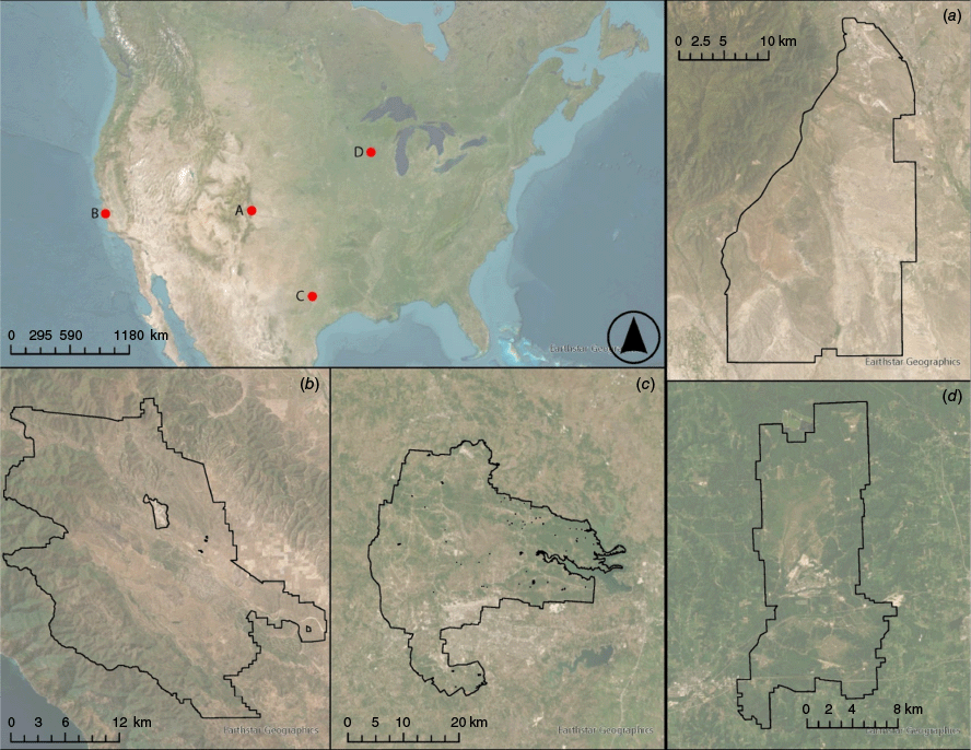
We selected four military installations within CONUS that represent different physiographic regions (Bailey 1980), vegetation types (Rollins 2009; Dewitz and U.S. Geological Survey 2021) and pyromes (Cattau et al. 2022, Table 1): Fort Carson (38.709°N 104.772°W) in Colorado Springs, Colorado; Fort Cavazos (31.195°N, 97.741°W) in Killeen, Texas; Fort Hunter Liggett (35.952°N 121.23065°W) in Monterey, California; and Fort McCoy (44.013°N, 90.688°W) in Tomah, Wisconsin (Fig. 1). The installations cover three different pyromes, which are spatial delineations characterized by general fire occurrence, size and severity patterns across CONUS (Cattau et al. 2022). Fort Hunter Liggett is in Pyrome 6, which is characterized by high intensity fires, relatively low human ignition sources (less than 17%) and a fire return interval ranging between 35–200 years. Fort Cavazos and Fort Carson are both located in Pyrome 8, which is characterized by human-caused fires, a relatively long fire season with low to moderate severity and a return interval of less than 35 years. Fort McCoy is in Pyrome 3, which, like Pyrome 8, is characterized by anthropogenic fires. The fire intensity is moderate, and the frequency is relatively low but has recently shown high rates of increase.
| Study Site | Size | Location | Physiographic provinces (Bailey 1980) | Vegetation types (Rollins 2009; Dewitz and U.S. Geological Survey 2021) | Pyrome (Cattau et al. 2022) | |
|---|---|---|---|---|---|---|
| Fort Carson | 558 km2 | Colorado Springs, CO | Dry steppes Province | Great Plains Shortgrass Prairie, Southern Rocky Mountain Pinyon-Juniper Woodlands and Northern Great Plains Mesic Mixed Grass Prairie Grassland. | 8. Long fire season with moderate frequency and intensity. 90% of annual fires due to anthropogenic activities. | |
| Fort Hunter Liggett | 650 km2 | Monterey, CA | Mediterranean Hard-leaved evergreen forests, open woodlands and shrub | California Xeric Chaparral, California Broadleaf Forest and Woodland and California Ruderal Grassland and Meadow. | 6. High intensity fires, relatively low human ignition sources (less than 17%) and a fire return interval ranging between 35–200 years. | |
| Fort Cavazos | 561 km2 | Killeen, TX | Shortgrass Steppes | Southern Plateau Dry Forest and Woodland, Great Plains Comanchian Ruderal Shrubland and Great Plains Comanchian Ruderal Grassland. | 8. Long fire season with moderate frequency and intensity. 90% of annual fires due to anthropogenic activities. | |
| Fort McCoy | 242 km2 | Tomah, WI | Wisconsin Mixed Wood Plains | North-Central Oak – Hickory Forest and Woodland, Northern and Central Ruderal Meadow, North-Central Oak Savanna and Barrens. | 3. Moderate human-started fires. Shows a high rate of increase in fire frequency (1980s – present). |
Study site maps for (a) Fort Carson (38.709°N 104.771°W), (b) Fort Hunter Liggett (35.952°N 121.230°W), (c) Fort Cavazos (31.195°N, 97.741°W), and (d) Fort McCoy (44.013°N, 90.688°W).
Despite being ecologically different, the installations included in this study have many commonalities; all four installations are multi-use landscapes with heterogeneous vegetation physiognomy. A large portion of herbaceous areas on each site are utilized as training ranges, where live firing activities occur and large machinery is operated. Exposure to these training exercises results in higher ignition rates in these areas and increased likelihood of wildfires. To mitigate risks from wildfires, the Army has fire breaks in place and performs annual prescribed burns on several installation in areas of high risk (Price and Bourne 2011).
Data acquisition and processing
We downloaded all available atmospherically corrected Landsat imagery from 1984 to 2023 (Landsat 5 TM = 1984–2012, Landsat 7 ETM + =2013, Landsat 8 OLI=2014–2023) that contained less than 15% cloud cover from Google Earth Engine’s (GEE) surface reflectance dataset (Gorelick et al. 2017; U.S. Geological Survey 2015) to create a time series. We masked clouds, cloud shadows and snow using the pixel quality assurance band (“QA_PIXEL”) included with each image and rescaled the images according to US Geological Survey (USGS) protocol (*0.0000275–0.2; Sayler and Zanter 2021). If 30% or more of an image’s pixels (30 m × 30 m) were No Data values, we removed the image from analysis. For each image in the time series, we calculated Normalized Difference Vegetation Index (NDVI), the tasseled cap indices for wetness, brightness and greenness, which provide a simplified representation of the spectral characteristics of vegetation (Kauth and Thomas 1976), tasseled cap angle (Powell et al. 2010), tasseled cap distance (Duane et al. 2010) and three burn indices: the NBR, the BAI and the MIRBI (Table 2). In addition, we calculated the difference from average in NBR, BAI and MIRBI (ΔNBR, ΔBAI and ΔMIRBI) for each image by subtracting the current value at each pixel from the mean value at that pixel for the entire time series. Finally, we Z-score standardized each burn index by subtracting each pixel value from the overall mean value of the image’s pixels and dividing by the standard deviation of the image’s pixels (ΔNBRZ, ΔBAIZ and ΔMIRBIZ; Table 2). All calculated findices were added as a band to the original Landsat images, which were then used for processing in both the validation dataset and ML algorithms.
| Band/Index | Formula | Source | |
|---|---|---|---|
| Blue (0.45–0.52 µm) | Landsat 5\7: Band 1 | ||
| Landsat 8: Band 2 | |||
| Green (0.52–0.60 µm) | Landsat 5\7: Band 2 | ||
| Landsat 8: Band 3 | |||
| Red (0.63–0.69 µm) | Landsat 5\7: Band 3 | ||
| Landsat 8: Band 4 | |||
| Near infrared (NIR) (0.76–0.90 µm) | Landsat 5\7: Band 4 | ||
| Landsat 8: Band 5 | |||
| Shortwave infrared 1 (SWIR1) (1.55–1.75 µm) | Landsat 5\7: Band 5 | ||
| Landsat 8: Band 6 | |||
| Shortwave infrared 2 (SWIR2) (2.08–2.55 µm) | Landsat 5\7: Band 7 | ||
| Landsat 8: Band 7 | |||
| Normalized difference vegetation Index (NDVI) | (NIR – Red)/(NIR + Red) | Tucker (1979) | |
| Tasseled cap | See source (formula is very long) | Kauth and Thomas (1976) | |
| Tasseled Cap Angle (TCA) | Arctan(Greenness/Brightness) | Powell et al. (2010) | |
| Tasseled Cap Distance (TCD) | Duane et al. (2010) | ||
| Normalized Burn Ratio (NBR) | (NIR – SWIR2) / (NIR + SWIR2) | López García and Caselles (1991) | |
| ΔNBRZ | (NBR – (mean(NBR))) – std(NBR) | ||
| Burned Area Index (BAI) | 1/(0.1 − Red)2 + (0.6 − NIR) | Chuvieco et al. (2002) | |
| ΔBAIZ | (BAI – (mean(BAI))) – std(BAI) | ||
| Mid Infrared Burn Index (MIRBI) | SWIR2 × 10 − (NIR × 9.8) + 2 | Trigg and Flasse (2001) | |
| ΔMIRBIZ | (MIRBI – (mean(MIRBI))) – std(MIRBI) |
Validation dataset generation and summarization
We produced validation datasets for each installation from 1984 to 2023 based on each pixel’s ΔMIRBIZ value using Python version 3.9.11 and ArcGIS Pro version 3.1.0 (ESRI, inc. 2022). We set a threshold of ΔMIRBIZ ≥2 to classify each pixel as burned (Value = 1) or not burned (Value = 0). Though sufficient for detecting both forest and grassland fires at each installation, this threshold misclassified other land disturbances (e.g. flooding, tilling, crop harvest and shadows) as burned area (average commission error of 0.63). To correct for these misclassifications, all images were converted to polygons, visually corrected by hand using false color images (near infrared (NIR), red, green) for reference (Masek et al. 2006; Wulder et al. 2012) and converted back to a raster in the original projection. For each pixel in a time series for each year, we classified the pixel as either unburned (value = 0) or burned (value = 1). This summary corrected for burned areas persisting over multiple images but assumed that each pixel burned no more than once per year.
We used the polygons to summarize burned area by month for each of the installations. We combined the annual summaries into a single raster for each installation representing total count of burns in each pixel from 1984 to 2023. Mean burned area count was determined through taking the average burned area count per pixel at each installation. We utilized the final shapefiles associated for each Landsat image to calculate annual burned area (ha), total area and identify first date of burn detection. To quantify the proportion of fires occurring near military ranges, we generated a 500 m buffer around all ranges, summarized burned area within and divided by total burned area. We defined fire season length for each installation by taking the standard deviation of Julian calendar days with fire present and multiplying it by two (Cattau et al. 2022). We also tested for significant (α = 0.05) change in yearly burned area over time with a simple linear regression model.
Model development and evaluation
We ran both the RF and XGBoost models in Python using Scikit-learn packages: RandomForestClassifier and XGboost (Van Rossum and Drake 1995; Pedregosa et al. 2011). For each study site, we generated RF and XGBoost models for both Landsat 5/7 and Landsat 8 imagery (four total) due to the satellites’ differences in bands and sensors. We trained and tested both the RF and XGBoost models with the same 10 images from each validation dataset, five from Landsat 5 and five from Landsat 8. The 10 images were chosen based on the presence of fire (over 100 ha), the image quality (90% of pixels present) and season in which the image was taken (at least one from each season). From each image, we sampled 700 pixels, 400 unburned and 300 burned. We randomly assigned half of the stratified sample points from each image as training or testing points. Each sample point had the classification (burned or unburned), the original Landsat band values and pixel values for each index described in Table 2. We recorded the importance values, or the proportional number of times each predictor is used to split data across each tree, with corresponding Scikit-learn packages (Van Rossum and Drake 1995; Pedregosa et al. 2011).
Each RF model was made with 200 estimators (trees). The hyperparameters tested in each RF model were the maximum number of predictors used at each leaf node and the maximum depth of each tree. Several options were tested for each hyperparameter (Supplementary Table S1), and the most successful combination was used in the final model. Each XGBoost model was made with 1000 estimators (trees). The hyperparameters tested in each XGBoost model are the learning rate, the maximum depth of each tree, the maximum child weight, gamma, subsample, column sample by tree and the regular alpha. Several options were tested (Supplementary Table S2) for each hyperparameter, and the most successful combination was used in the final, optimized model.
The optimized models were applied to the remainder of the Landsat imagery with the calculated indices included as bands. The resulting raster data set consisted of each pixel’s probability of representing a burn scar on a scale of 0–1. To correct for burn scars persisting over multiple images, especially those that remain into the next calendar year, each burned area raster was compared to the previous in the time series, and if both rasters had fire present in the same pixel (probability >75%), the second raster’s pixel was reassigned as not burned (0). We summarized the raster data set by taking the maximum pixel value of images for each year.
Sampling for validation included generating 1000 stratified (based on validation dataset burn values) random points for each year, we then filtered these points to maintain a minimum distance of 500 m between points. Validation value, RF likelihood, XGBoost likelihood and the predictor values for each point were recorded. We compared confusion matrices, commission/omission error rates, specificity values, sensitivity values and total accuracy calculated with R’s Caret package (Kuhn 2008; R Core Team 2023) at various likelihoods for each model. Each model’s optimum likelihood threshold was determined by the highest total accuracy recorded when tested in increments of 5 (5, 10, […] 95, 100%). We classified each installations’ yearly rasters at their respective optimum threshold and combined them to represent total count of burns in each pixel from 1984 to 2023.
RF and XGBoost model results for each site were first tested for significant differences using the McNemar’s Chi-squared test for paired categorical data (Fagerland et al. 2013). If significantly different, we used overall accuracy to determine which algorithm was most successful at each study site. To further explore where errors were occurring, we calculated difference maps by subtracting the final burn count raster of both ML algorithms from the validation dataset burn count rasters (Raster Calculator, ESRI, inc. 2022). The difference maps were randomly sampled, and error value and groundcover value (Dewitz and U.S. Geological Survey 202) associated with each sampling point were recorded. We performed all statistical analyses in the R statistical platform (R Core Team 2023). Scripts are available upon request.
Results
Validation dataset
We used an average of 210 images (128–246 range) per installation (1984–2023; Supplementary Table S3). Within individual installations, there was large variability in burn occurrences (Fig. 2), with the total number of burns from 1984–2023 being greatest near training ranges. On Fort Carson, 90% of detected burned area was within 500 m of firing ranges and impact areas. The number were similar for Fort Cavazos (94%) and Fort McCoy (98%). On Fort Hunter Liggett, only ~20% of detected burned areas were within 500 m of firing ranges due to the high occurrence of prescribed fire performed on the site. On Fort Carson, the highest count (located on a training impact area) was 11 burns from 1984 to 2023. On Fort Hunter Liggett the highest count (located on a designated prescribed burn unit) was 28 burns; on Fort Cavazos, the highest count (located on a live fire training area) was 15 burns; on Fort McCoy, the highest count (located on a training impact area) was 11 burns. All four installations had significant area (>30% of the installation) that did not burn at all within the entire time series.
Validation (I), random forest (RF) (II) and XGBoost (III) burned area count results for all four Installations: Fort Carson (a), Fort Hunter Liggett (b), Fort Cavazos (c), and Fort McCoy (d). Burn count represents the number of years each pixel was identified as burned from 1984–2023.
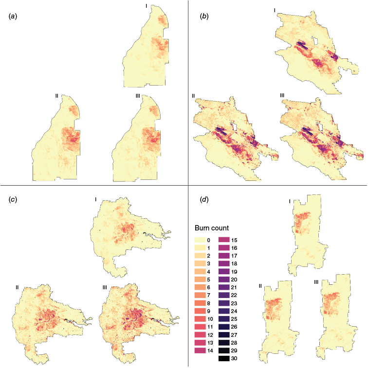
The study site with the highest average burned area per year was Fort Hunter Liggett (2596 ha year−1) followed by Fort Carson (2093 ha year−1), then Fort Cavazos (1660 ha year−1) and finally Fort McCoy (377 ha year−1). Fort Hunter Liggett had the shortest fire season length of 114 days with most fires occurring in the summer months. June had the highest average burned area (~750 ha) with February, March and April having the lowest (0 ha). Fort McCoy had a slightly longer fire season of 153 days, with most fires occurring in the spring. The highest average burned area on Fort McCoy was in April (~200 ha) and the lowest was in January (0 ha). Fort Cavazos and Fort Carson had the longest fire season lengths of 213 and 233 days respectively, with fires occurring in all seasons with a heavy emphasis on spring and fall. Fort Cavazos had the highest average burned area in August (>650 ha) and the lowest in May (<20 ha). Fort Carson had the highest average burned area in December (>450 ha) and the lowest in July (<50 ha). Burned area count did not change through time (years) for Fort Carson, Fort Hunter Liggett or Fort Cavazos (P > 0.05), but burned area did increase at Fort McCoy through time (slope = 23.8, P < 0.001).
Machine learning
Hyperparameter optimization results for both the RF and the XGBoost models varied across installations and Landsat satellite systems (Supplementary Tables S1 and S2). For the RF models, the most common number of predictors for the optimized model was six, while the most common maximum depth optimized parameter was nine. For the XGBoost models, the optimized maximum depth parameter was quite variable, with all tested values being identified at least once. The minimum child weight of one was identified on all but one model, and a learning rate of either 0.01 or 0.05 was the optimal parameter for all models. The optimized gamma values were either 0.3 or 0.4, depending on the model. Both subsample values and column samples per tree varied with no particular value being preferred. In the current study, parameter optimization had little effect on model performance, with range of accuracy values being 0.96 to 0.99 in both the RF and XGboost models.
Overall, ΔMIRBIZ had the highest importance value across installations and satellite systems, ranging from 0.213 to 0.778 (Supplementary Table S4). Other variables with high importance values were ΔNBRZ (0.003–0.306), MIRBI (0.037–0.155) and NBR (0.011–0.214). TCA (0–0.153) and NDVI (0.001–0.138) showed importance in Fort Cavazos’s models and ΔBAIZ (0.003–0.153) showed relative importance in Fort McCoy’s. It is important to note that some predictors used in these models are correlated, so the importance values may be influenced by collinearity.
Both RF and XGBoost models had a wide range of optimum thresholds for classification (Table 3), most likely due to differences in landcover as well as training samples. We found RF to have an average optimum threshold of 63.75% likelihood, with the lowest being Fort Cavazos at 45% likelihood and the highest being Fort Carson and Fort McCoy at 75% likelihood. The average optimum threshold for XGBoost model classification was at 61.25% likelihood, with Fort Cavazos’s having the lowest at 15% and Fort Carson’s having the highest with 95%.
| Threshold | Accuracy | Omission | Commission | Sensitivity | Specificity | |
|---|---|---|---|---|---|---|
| Fort Carson | ||||||
| RF | ||||||
| 70% | 0.934 | 0.042 | 0.225 | 0.965 | 0.739 | |
| 75% | 0.935 | 0.047 | 0.197 | 0.972 | 0.704 | |
| 80% | 0.934 | 0.052 | 0.172 | 0.978 | 0.666 | |
| XGBoost | ||||||
| 90% | 0.933 | 0.039 | 0.241 | 0.961 | 0.760 | |
| 95% | 0.936 | 0.045 | 0.198 | 0.972 | 0.714 | |
| 99% | 0.928 | 0.065 | 0.145 | 0.984 | 0.578 | |
| Fort Hunter Liggett | ||||||
| RF | ||||||
| 55% | 0.947 | 0.021 | 0.151 | 0.952 | 0.930 | |
| 60% | 0.948 | 0.024 | 0.143 | 0.956 | 0.920 | |
| 65% | 0.947 | 0.029 | 0.134 | 0.960 | 0.903 | |
| XGBoost | ||||||
| 45% | 0.941 | 0.026 | 0.160 | 0.950 | 0.911 | |
| 50% | 0.943 | 0.028 | 0.151 | 0.953 | 0.906 | |
| 55% | 0.941 | 0.033 | 0.146 | 0.956 | 0.888 | |
| Fort Cavazos | ||||||
| RF | ||||||
| 40% | 0.930 | 0.035 | 0.241 | 0.951 | 0.818 | |
| 45% | 0.933 | 0.040 | 0.216 | 0.960 | 0.788 | |
| 50% | 0.926 | 0.055 | 0.190 | 0.970 | 0.696 | |
| XGBoost | ||||||
| 10% | 0.916 | 0.033 | 0.306 | 0.932 | 0.829 | |
| 15% | 0.919 | 0.042 | 0.273 | 0.946 | 0.777 | |
| 20% | 0.913 | 0.056 | 0.263 | 0.953 | 0.698 | |
| Fort McCoy | ||||||
| RF | ||||||
| 70% | 0.947 | 0.038 | 0.186 | 0.979 | 0.699 | |
| 75% | 0.948 | 0.042 | 0.154 | 0.984 | 0.668 | |
| 80% | 0.946 | 0.047 | 0.135 | 0.987 | 0.629 | |
| XGBoost | ||||||
| 80% | 0.939 | 0.044 | 0.218 | 0.976 | 0.654 | |
| 85% | 0.941 | 0.047 | 0.180 | 0.982 | 0.625 | |
| 90% | 0.941 | 0.052 | 0.139 | 0.988 | 0.581 | |
Both the RF and XGBoost models showed relative success at delineating burn areas in the Landsat time series. The RF total accuracies ranged from 0.933 for Fort Cavazos to 0.948 for Fort McCoy and Fort Hunter Liggett (Table 3). The mean RF omission error across all four sites was 0.053, with Fort Hunter Liggett having the lowest (0.024) and Fort Carson having the highest (0.047). The mean RF commission error was 0.178, with Fort Hunter Liggett having the lowest (0.143) and Fort Cavazos having the highest (0.216). The XGBoost models’ total accuracies ranged from 0.919 for Fort Cavazos to 0.943 for Fort Hunter Liggett. The mean XGBoost omission error was 0.041 with Fort Hunter Liggett having the lowest (0.028) and Fort McCoy having the highest (0.047). The mean XGBoost commission error was 0.200 with Fort Hunter Liggett having the lowest (0.151) and Fort Cavazos having the highest (0.273). Confusion matrices for each installation can be seen in Table 4 and the geospatial fire history results can be seen in Fig. 2.
| Validated 0 | Validated 1 | Validated 0 | Validated 1 | ||
|---|---|---|---|---|---|
| Fort Carson | Fort Hunter Liggett | ||||
| RF 0 | 10,734 | 528 | 12,526 | 302 | |
| RF 1 | 308 | 1254 | 580 | 3491 | |
| XGBoost 0 | 10,729 | 510 | 12,494 | 356 | |
| XGBoost 1 | 313 | 1272 | 612 | 3437 | |
| Fort Cavazos | Fort McCoy | ||||
| RF 0 | 15,168 | 626 | 6044 | 265 | |
| RF 1 | 639 | 2326 | 97 | 532 | |
| XGBoost 0 | 14,946 | 659 | 6032 | 299 | |
| XGBoost 1 | 861 | 2283 | 109 | 498 | |
Each matrix includes pixel count of true false (Model 0 and Validated 0), true true (Model 1 and Validation 1), omission count (Model 0 and Validated 1) and commission count (Model 1 and Validated 0) resulting from validation samples.
The RF and XGBoost results at optimal thresholds were not found to be statistically different according to McNamar’s test, apart from Fort Cavazos (P-value < 0.001) where RF outperformed XGBoost at delineating burned areas (R Core Team 2023). However, when the threshold was standardized across models at 75% likelihood, McNamar’s test resulted in an average P-value < 0.001. At 75% likelihood, RF outperformed XGBoost in three out of the four locations: Fort Carson, Fort Cavazos and Fort McCoy. Fort Hunter Liggett’s XGBoost model outperformed its RF model at 75% likelihood in delineating burn area.
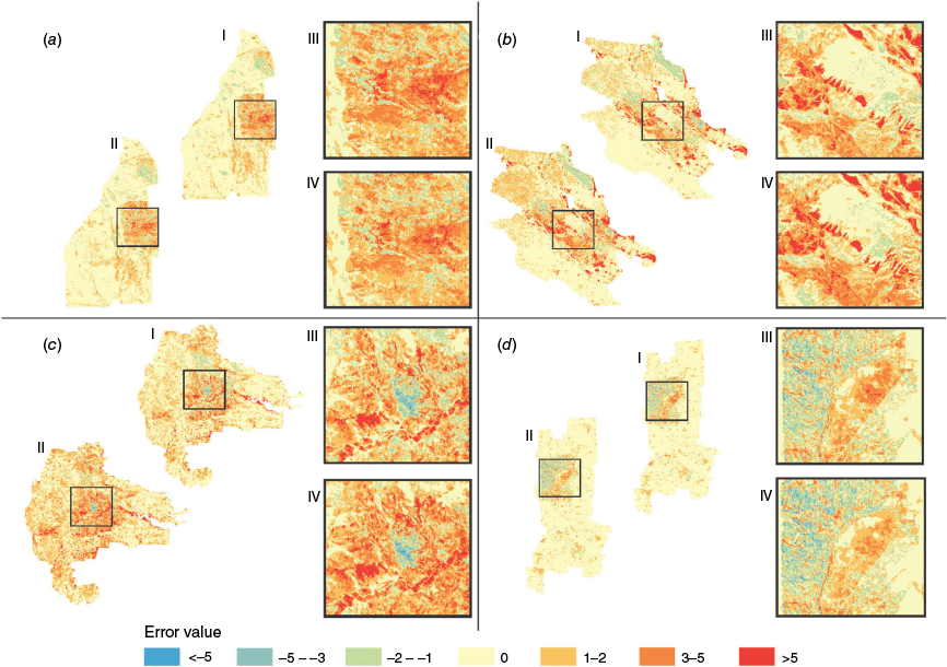
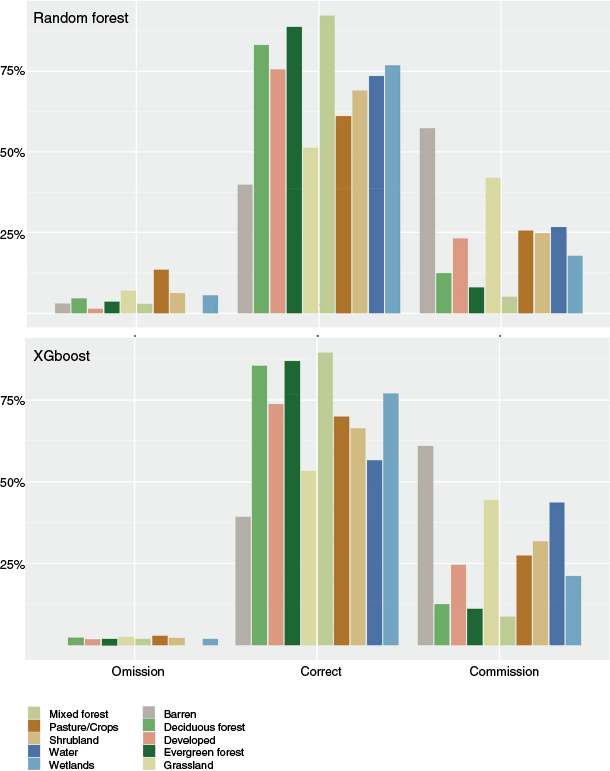
Across the four study areas, omission and commission errors were spatially variable. At each of the four study sites, there were pixel clusters repeatedly being missed (omitted) or incorrectly flagged (committed, Fig. 3) as burned area across the time series. Fort Carson, Fort Hunter Liggett and Fort Cavazos show a higher rate of commission errors, with certain pixel clusters being incorrectly flagged >5 times throughout the timeseries. Fort McCoy shows a higher rate of omission, comparatively, with pixel clusters being missed >3 times. The landcovers (Fig. 4) associated with commission errors across both RF and XGBoost models are barren land, grasslands, open water, shrubland, cropland and developed areas. The RF models tended to have a higher rate of omission as compared to XGBoost, with the main landcover class associated with those errors being pasture and cropland.
Difference Values (machine learning (ML) results – validation dataset) for each study site: Fort Carson (a), Fort Hunter Liggett (b), Fort Cavazos (c), and Fort McCoy (d). Each study site shows random forest (RF) difference values (I) with a closeup of errors (III), and XGBoost difference values (II) with a closeup of errors (IV). Error values represent the difference between the ML results and the validation dataset, with negative values representing omission errors and positive values representing commission errors.
Omission and Commission error count by landcover type (Dewitz and U.S. Geological Survey 2021). Count was determined through random sampling of difference rasters (Fig. 3) and associated landcover as described by the National Landcover Dataset.
Discussion
Accurate estimates of fire history are important for understanding historical fire regimes, assessing fire susceptibility and understanding threats to civil, cultural and natural resources. We were able to successfully combine Landsat satellite imagery with two ML algorithms, RF and XGBoost, to delineate burned areas in a decadal time series (1984–2023) and to reconstruct local fire histories across four US military installations in the US. Our analysis produced favorable results; the mean accuracy for the RF models across all four installations was 0.941, the mean accuracy of XGBoost was 0.935, and the average sensitivity value across models was 0.97. The methodology presented in this paper can provide a framework for accurately summarizing fire history at the local scale, paramount for areas with unique fire histories like military installations.
Overall, both the RF and XGBoost models performed similarly. Recent studies (Lee et al. 2019; Sahin 2020; Shao et al. 2024) have reported XGBoost outperforming RF in satellite imagery classification. The success of the ML algorithms in the current study may be attributed to the scale at which the models were applied, or the use of site-specific training/testing datasets to avoid over-fitting (Kuhn and Johnson 2013). Global/national burn area estimations (Hawbaker et al. 2017; Ramo and Chuvieco 2017; Giglio et al. 2018) use several local scale training areas, and then apply the model at larger scales, increasing the chance of over-fitting. As a result, they have relatively large omission errors (0.23–0.43) in comparison to our models. Our models also outperformed studies done on regional scales utilizing ML algorithms to delineate burn scars (Liu et al. 2018; Goodwin and Collett 2014) which had accuracy rates of 79.2 and 80.0% respectively.
Our unique validation dataset, which included the entire time series, allowed us to get a more accurate estimation of model success and find patterns of errors that can aid in improving future methodologies. One pattern we found with our validation dataset was that all models outperformed the original ΔMIRBIZ threshold of two (commission errors ranging from 0.40 to 0.78) in discriminating burn scars from other landscape disturbances. Though our models outperformed ΔMIRBIZ alone, we recognize the need for improvement in lowering commission error as certain landcovers and disturbances were continuously misclassified as burn scars. Fort Cavazos (Texas) in particular had consistently high commission errors for both models, which may be due to the heterogeneous landscape of the installation, and the presence of large patches of bare soil. Commission error has been addressed in numerous ways in the literature, but a common approach is masking for landcovers often misclassified as burned area, such as agricultural plots, water bodies and urban areas. These landcovers are difficult to distinguish from fires remotely as they have similar spectral characteristics, and future studies may benefit from modeling different landcovers separately or feeding models information regarding landcover type. Discriminating between burn scars and other disturbances is a current gap in literature that needs to be addressed to avoid high commission errors in multiuse landscapes such as wildland–urban interfaces and military installations.
All four study sites demonstrated spatial variation in fire frequency, where a large percentage (0.2–0.98) of fires occurred in or around military training ranges. This was expected as fuel characteristics and exposure to ignition sources increases risk of fire in these areas. Though the fire season length of each installation was comparable to the pyrome characteristics described in Cattau et al. 2022, we found that the fire frequency on training ranges were higher than expected, though the image resolution (30 m) may be detecting smaller fires not considered in Cattau’s study, which uses MODIS (500 m). It is also important to note that fire occurrences on these landscapes are heavily influenced by anthropogenic activities. For example, Fort Carson had many fires occurring in winter months, outside the fire season associated with its surrounding pyrome. Future studies exploring fire occurrences on military land, particularly the weather patterns associated with ignitions, would aid in understanding how land usage is affecting the vulnerability of these landscapes.
Conclusion
The methodology presented in this study proved to be successful using both a RF and XGBoost model. The direct results of this study can be used by each site’s respective management personnel in determining preventative measures (if needed) and assessing risk moving forward. The four installations used in this study cover a range of ecosystems and pyromes, however, there is still a need to test the methodology on other physiographic regions. US military installations can be found in all 50 states, as well as numerous locations in Africa, Asia, Europe and South America. Further validation of the methodology on installations in various regions would support testing how model success and vegetation/fire index performance vary across the globe. This ground up approach can be utilized by other Army personnel and local land managers to assess the contemporary burned area history on other sites. Local knowledge is key to successful management, and we present an accessible methodology to develop fire histories for local-scale management units, particularly those geared towards national defense institutions.
Declaration of funding
The authors recognize generous support from the US Army Engineer Research and Development Center (ERDC) and the 335 Installations and Operational Environments (IOE) 6.2–6.3 program funding under the Intelligent Environmental 336 Battlefield Awareness (IEBA), Extreme Environmental Impacts on Military Operations work package.
Acknowledgements
The authors are thankful for the help of the Training Lands team at the US Army Research and Development Center’s 328 (ERDC) Construction Engineering Research Laboratory (CERL).
References
Ager AA, Day MA, Alcasena FJ, Evers CR, Short KC, Grenfell I (2021) Predicting paradise: modeling future wildfire disasters in the western US. The Science of The Total Environment 784, 147057.
| Crossref | Google Scholar | PubMed |
Belgiu M, Drăguţ L (2016) Random forest in remote sensing: a review of applications and future directions. ISPRS Journal of Photogrammetry and Remote Sensing 114, 24-31.
| Crossref | Google Scholar |
Bot K, Borges JG (2022) A systematic review of applications of machine learning techniques for wildfire management decision support. Inventions 7(1), 15.
| Crossref | Google Scholar |
Breiman L (2001) Random forests. Machine Learning 45, 5-32.
| Crossref | Google Scholar |
Calkin DE, Thompson MP, Finney MA (2015) Negative consequences of positive feedbacks in US wildfire management. Forest Ecosystems 2, 1-10.
| Crossref | Google Scholar |
Cattau ME, Mahood AL, Balch JK, Wessman CA (2022) Modern pyromes: biogeographical patterns of fire characteristics across the contiguous United States. Fire 5(4), 95.
| Crossref | Google Scholar |
Chen T, Guestrin C (2016) Xgboost: A scalable tree boosting system. In ‘Proceedings of the 22nd ACM SIGKDD International Conference on Knowledge Discovery and Data Mining’. pp. 785–794. (Association for Computing Machinery: New York, NY, USA). 10.1145/2939672.2939785
Chuvieco E, Martín MP, Palacios A (2002) Assessment of different spectral indices in the red-near-infrared spectral domain for burned land discrimination. International Journal of Remote Sensing 23(23), 5103-5110.
| Crossref | Google Scholar |
Chuvieco E, Aguado I, Salas J, García M, Yebra M, Oliva P (2020) Satellite remote sensing contributions to wildland fire science and management. Current Forestry Reports 6, 81-96.
| Crossref | Google Scholar |
Conedera M, Tinner W, Neff C, Meurer M, Dickens AF, Krebs P (2009) Reconstructing past fire regimes: methods, applications, and relevance to fire management and conservation. Quaternary Science Reviews 28(5-6), 555-576.
| Crossref | Google Scholar |
Dewitz J, U.S. Geological Survey (2021) National Land Cover Database (NLCD) 2019 Products (ver. 2.0, June 2021): U.S. Geological Survey data release. 10.5066/P9KZCM54
Duane MV, Cohen WB, Campbell JL, Hudiburg T, Turner DP, Weyermann DL (2010) Implications of alternative field-sampling designs on Landsat-based mapping of stand age and carbon stocks in Oregon forests. Forest Science 56(4), 405-416.
| Crossref | Google Scholar |
Fagerland MW, Lydersen S, Laake P (2013) The McNemar test for binary matched-pairs data: mid-p and asymptotic are better than exact conditional. BMC Medical Research Methodology 13, 91.
| Crossref | Google Scholar | PubMed |
Forsyth GG, Van WBW (2008) The recent fire history of the Table Mountain National Park and implications for fire management: original research. Koedoe : African Protected Area Conservation and Science 50, 3-9.
| Crossref | Google Scholar |
Freeman J, Kobziar L, Rose EW, Cropper W (2017) A critique of the historical-fire-regime concept in conservation. Conservation Biology 31, 976-985.
| Crossref | Google Scholar | PubMed |
Gavin DG, Hu FS, Lertzman K, Corbett P (2006) Weak climatic control of stand‐scale fire history during the late Holocene. Ecology 87(7), 1722-1732.
| Crossref | Google Scholar | PubMed |
Giglio L, Boschetti L, Roy DP, Humber ML, Justice CO (2018) The Collection 6 MODIS burned area mapping algorithm and product. Remote Sensing of Environment 217, 72-85.
| Crossref | Google Scholar | PubMed |
Goodwin NR, Collett LJ (2014) Development of an automated method for mapping fire history captured in Landsat TM and ETM+time series across Queensland, Australia. Remote Sensing of Environment 148, 206-221.
| Crossref | Google Scholar |
Gorelick N, Hancher M, Dixon M, Ilyushchenko S, Thau D, Moore R (2017) Google Earth Engine: planetary-scale geospatial analysis for everyone. Remote Sensing of Environment 202, 18-27.
| Crossref | Google Scholar |
Hawbaker TJ, Vanderhoof MK, Beal YJ, Takacs JD, Schmidt GL, Falgout JT, Williams B, Fairaux NM, Caldwell MK, Picotte JJ, Howard SM, Stitt S, Dwyer JL (2017) Mapping burned areas using dense time-series of Landsat data. Remote Sensing of Environment 198, 504-522.
| Crossref | Google Scholar |
Hawbaker TJ, Vanderhoof MK, Schmidt GL, Beal YJ, Picotte JJ, Takacs JD, Falgout JT, Dwyer JL (2020) The Landsat Burned Area algorithm and products for the conterminous United States. Remote Sensing of Environment 244, 111801.
| Crossref | Google Scholar |
Hearst MA, Dumais ST, Osuna E, Platt J, Scholkopf B (1998) Support vector machines. IEEE Intelligent Systems and their Applications 13, 18-28.
| Crossref | Google Scholar |
Hoffmann WA, Orthen B, Nascimento PKVd (2003) Comparative fire ecology of tropical savanna and forest trees. Functional Ecology 17(6), 720-726.
| Crossref | Google Scholar |
Hohmann MG, Wall WA, Just MG, Huskins SD (2023) Multiple intrinsic and extrinsic drivers influence the quantity and quality components of seed dispersal effectiveness in the rare shrub Lindera subcoriacea. PLoS One 18, e0283810.
| Crossref | Google Scholar | PubMed |
Just MG, Hohmann MG, Hoffmann WA (2016) Where fire stops: vegetation structure and microclimate influence fire spread along an ecotonal gradient. Plant Ecology 217, 631-644.
| Crossref | Google Scholar |
Just MG, Wall WA, Huskins SD, Hohmann MG (2024) Effects of landscape heterogeneity and disperser movement on seed dispersal. Ecologies 5(2), 198-217.
| Crossref | Google Scholar |
Kauth RJ, Thomas GS (1976) The Tasselled Cap—A Graphic Description of the Spectral-Temporal Development of Agricultural Crops as Seen by LANDSAT. (LARS Symposia) http://docs.lib.purdue.edu/lars_symp/159
Kelly LT, Bennett AF, Clarke MF, McCarthy MA (2015) Optimal fire histories for biodiversity conservation. Conservation Biology 29, 473-481.
| Crossref | Google Scholar | PubMed |
Krebs P, Pezzatti GB, Mazzoleni S, et al. (2010) Fire regime: history and definition of a key concept in disturbance ecology. Theory in Biosciences 129, 53-69.
| Crossref | Google Scholar | PubMed |
Kuhn M (2008) Building predictive models in R using the caret package. Journal of Statistical Software 28(5), 1-26.
| Crossref | Google Scholar |
Kuhn M, Johnson K (2013) ‘Applied Predictive Modeling.’ (Springer: New York, NY, USA). 10.1007/978-1-4614-6849-3
Kyser GB, Wilson RG, Zhang J, DiTomaso JM (2013) Herbicide-assisted restoration of Great Basin sagebrush steppe infested with medusahead and downy brome. Rangeland Ecology & Management 66(5), 588-596.
| Google Scholar |
Leach MK, Givnish TJ (1999) Gradients in the composition, structure, and diversity of remnant oak savannas in southern Wisconsin. Ecological Monographs 69(3), 353-374.
| Crossref | Google Scholar |
Lee Y, Han D, Ahn MH, Im J, Lee SJ (2019) Retrieval of total precipitable water from Himawari-8 AHI data: a comparison of random forest, extreme gradient boosting, and deep neural network. Remote Sensing 11(15), 1741.
| Crossref | Google Scholar |
Likas A, Vlassis N, Verbeek JJ (2003) The global k-means clustering algorithm. Pattern Recognition 36, 451-461.
| Crossref | Google Scholar |
Liu J, Heiskanen J, Maeda EE, Pellikka PK (2018) Burned area detection based on Landsat time series in savannas of southern Burkina Faso. International Journal of Applied Earth Observation and Geoinformation 64, 210-220.
| Crossref | Google Scholar |
López García MJ, Caselles V (1991) Mapping burns and natural reforestation using thematic Mapper data. Geocarto International 6(1), 31-37.
| Crossref | Google Scholar |
Marlon JR, Bartlein PJ, Gavin DG, Long CJ, Anderson RS, Briles CE, Brown KJ, Colombaroli D, Hallett DJ, Power MJ, Scharf EA, Walsh MK (2012) Long-term perspective on wildfires in the western USA. Proceedings of the National Academy of Sciences 109(9), 535-43.
| Crossref | Google Scholar | PubMed |
Masek JG, Vermote EF, Saleous NE, Wolfe R, Hall FG, Huemmrich KF, Lim TK (2006) A Landsat surface reflectance dataset for North America, 1990-2000. IEEE Geoscience and Remote Sensing Letters 3(1), 68-72.
| Crossref | Google Scholar |
Nagy RC, Fusco E, Bradley B, Abatzoglou JT, Balch J (2018) Human-related ignitions increase the number of large wildfires across US ecoregions. Fire 1(1), 4.
| Crossref | Google Scholar |
Pedregosa F, Varoquaux G, Gramfort A, Michel V, Thirion B, Grisel O (2011) Scikit-learn: machine learning in Python. Journal of Machine Learning Research 12, 2825-2830.
| Google Scholar |
Powell SL, Cohen WB, Healey SP, Kennedy RE, Moisen GG, Pierce KB, Ohmann JL (2010) Quantification of live aboveground forest biomass dynamics with Landsat time-series and field inventory data: a comparison of empirical modeling approaches. Remote Sensing of Environment 114(5), 1053-1068.
| Crossref | Google Scholar |
Price RA, Bourne M (2011) Effects of Wildfire and Prescribed Burning on Distributed Particles of Composition-B Explosive on Training Ranges. In ‘Environmental Chemistry of Explosives and Propellant Compounds in Soils and Marine Systems: Distributed Source Characterization and Remedial Technologies, Vol. 1069’. (Eds M Chappell, C Price, R George) pp. 363–377. (American Chemical Society) 10.1021/bk-2011-1069.ch019
Ramo R, Chuvieco E (2017) Developing a random forest algorithm for MODIS global burned area classification. Remote Sensing 9(11), 1193.
| Crossref | Google Scholar |
R Core Team (2023) R: A Language and Environment for Statistical Computing, Version 4.3.0. R Foundation for Statistical Computing, Vienna, Austria. Available at https://www.R-project.org/
Rollins MG (2009) LANDFIRE: a nationally consistent vegetation, wildland fire, and fuel assessment. International Journal of Wildland Fire 18(3), 235.
| Crossref | Google Scholar |
Roy DP, Huang H, Boschetti L, Giglio L, Yan L, Zhang HH, Li Z (2019) Landsat-8 and Sentinel-2 burned area mapping - A combined sensor multi-temporal change detection approach. Remote Sensing of Environment 231, 111254.
| Crossref | Google Scholar |
Royal EJ, Kross CS, Willson JD (2022) Legacy land use predicts occupancy patterns of prairie-associated herpetofauna in Western Arkansas. Landscape Ecology 38(2), 423-438.
| Crossref | Google Scholar |
Sahin EK (2020) Assessing the predictive capability of ensemble tree methods for landslide susceptibility mapping using XGBoost, gradient boosting machine, and random forest. SN Applied Sciences 2(7), 1308.
| Crossref | Google Scholar |
Santos JL, Hradsky BA, Keith DA, Rowe K, Senior KL, Sitters H, Kelly LT (2022) Beyond inappropriate fire regimes: a synthesis of fire-driven declines of threatened mammals in Australia. Conservation Letters 15, e12905.
| Crossref | Google Scholar |
Senande-Rivera M, Insua-Costa D, Miguez-Macho G (2022) Spatial and temporal expansion of global wildland fire activity in response to climate change. Nature Communications 13, 1208.
| Crossref | Google Scholar | PubMed |
Shao Z, Ahmad MN, Javed A (2024) Comparison of Random Forest and XGBoost Classifiers using Integrated Optical and SAR Features for mapping urban impervious surface. Remote Sensing 16(4), 665.
| Crossref | Google Scholar |
Stein BA, Scott C, Benton N (2008) Federal lands and endangered species: the role of military and other federal lands in sustaining biodiversity. BioScience 58(4), 339-347.
| Crossref | Google Scholar |
Syphard AD, Keeley JE (2015) Location, timing and extent of wildfire vary by cause of ignition. International Journal of Wildland Fire 24, 37-47.
| Crossref | Google Scholar |
Trigg S, Flasse S (2001) An evaluation of different bi-spectral spaces for discriminating burned shrub-savannah. International Journal of Remote Sensing 22(13), 2641-2647.
| Crossref | Google Scholar |
Tucker CJ (1979) Red and photographic infrared linear combinations for monitoring vegetation. Remote Sensing of Environment 8(2), 127-150.
| Crossref | Google Scholar |
U.S. Geological Survey (2015) Landsat surface reflectance data (ver. 1.1, 27 March, 2019). U.S. Geological Survey Fact Sheet 2015-3034, 1 p. 10.3133/fs20153034
Veraverbeke S, Lhermitte S, Verstraeten WW, Goossens R (2011) Evaluation of pre/post-fire differenced spectral indices for assessing burn severity in a Mediterranean environment with Landsat Thematic Mapper. International Journal of Remote Sensing 32(12), 3521-3537.
| Crossref | Google Scholar |
Wall WA, Hohmann MG, Just MG, Hoffmann WA (2021a) Characterizing past fire occurrence in longleaf pine ecosystems with the Mid-Infrared Burn Index and a Random Forest classifier. Forest Ecology and Management 500, 119635.
| Crossref | Google Scholar |
Wall WA, Walker AS, Gray JB, Hohmann MG (2021b) Fire effects on the vital rates and stochastic population growth rate of the rare shrub Lindera subcoriacea Wofford. Plant Ecology 222, 119-131.
| Crossref | Google Scholar |
Westerling AL, Hidalgo HG, Cayan DR, Swetnam TW (2006) Warming and earlier spring increase western US forest wildfire activity. Science 313(5789), 940-943.
| Crossref | Google Scholar | PubMed |
Wulder MA, Masek JG, Cohen WB, Loveland TR, Woodcock CE (2012) Opening the archive: how free data has enabled the science and monitoring promise of Landsat. Remote Sensing of Environment 122, 2-10.
| Crossref | Google Scholar |