The use of genomics in the management of livestock
B. P. KinghornUniversity of New England, Armidale, NSW 2351, Australia. Email: bkinghor@une.edu.au
Animal Production Science 52(3) 78-91 https://doi.org/10.1071/AN11092
Submitted: 30 May 2011 Accepted: 27 November 2011 Published: 6 March 2012
Journal Compilation © CSIRO Publishing 2012 Open Access CC BY-NC-ND
Abstract
Variation among animals exists at all stages of our livestock supply chains. In contrast, most manufacturing supply chains possess little, if any, unintended variation within each segment. This variation is generally an unwanted nuisance. However, when properly managed, it can provide opportunities to target multiple product end-points and turn-off dates in a dynamic manner. Moreover, optimal management can lead to high degrees of compliance with the needs of the processing segment of the supply chain and/or end-users. Management decisions can be divided into initial group formation (e.g. mating groups, feedlot entry groups) and ongoing changes to the management plan in the light of new information (including market forces, weather and genetic status of animals). In both cases, the best pattern of decision making depends, explicitly or implicitly, on the predicted effect of these decisions on future animal and processing performance. The present paper provides an overview of key factors that affect these predictions, and hence optimal management, and emphasises the potential role of genetic and genomic information for increasing focus and improving profitability in the beef supply chain.
Introduction
The present paper will focus on beef for illustration, but the principles apply across livestock species and products.
The production of beef and the supply chains that drive it differ from the corresponding components in the automotive industry. The key difference is variation – beef has extra variation in the production environment, the product, and in the pattern of management required to optimise profit, welfare and other outcomes.
The extra variation in management is compounded by the fragmented nature of the production system, where there is little power to predict the downstream effect of management interventions. If we halve the differential ratio in a car we will exactly double the speed per 1000 rpm; if we halve the stocking rate for beef cattle, we are unlikely to double the weight at slaughter.
Product variation is highly engineered across automotive assembly lines, with virtually no unintended variation between examples of the same model. We aim to engineer variation in the beef industry, using breeds and production systems appropriately. However, unlike cars, animals progressing along our beef assembly lines accumulate variations, whether or not the causes of these can be identified. We can exploit this extra variation opportunistically by changing turn-off dates, targeting different market end-points, and possibly reconstituting groups. This requires the ability to predict how animals will react to management interventions. Key requirements are data on animal status, including genetics, and robust models that predict animal performance as a function of management decisions.
We can separate beef management decisions somewhat loosely into the following two categories:
-
Choosing animals to enter the part of the supply chain concerned. Initial grouping decisions form animal resources at the start of the supply chain segment under consideration. This can be breed and sire choice in a cow–calf operation, or breed type and grouping decisions for entry into a feedlot. Such decisions are made in concert with a plan for management through to a market end-point at a target time, even if this is not the end of the supply chain.
-
Deciding the treatment and fate of animals that are already in the part of the supply chain concerned. Ongoing changes to the management plan can be made in light of new information, such as current and forecast weather, disease and mortalities, market fluctuations and new information on the genetic status of animals.
Genetics can play a role in both categories, at different levels such as breed, seed-stock source, use of heterosis, and estimates of breeding value (using pedigree and/or genetic markers). The present paper will consider the role of these genetic factors in making both initial and ongoing management decisions.
The impact of genetics on initial grouping decisions
All cattle destined for slaughter have to be managed to that end. The present paper does not address how to improve this overall population genetically – that is covered by animal breeders – but of course producers in the beef supply chain will compete to access animals that are most genetically appropriate for their businesses. The following two key factors are relevant here:
-
Merit – accessing appropriate levels of merit, due both to genetics and life-history environment, at appropriate cost.
Of relevance to the present paper is the ability to use genetics and genomics to help make these decisions. Components of potential relevance, for each commercially important trait, include breed type, breed, seed-stock source, sire, estimated breeding value from pedigree (EBV) and estimated breeding value from genomic information (gEBV, Goddard 2012).
-
Variation – forming management groups that are consistent, with minimal variation, to help achieve controlled management to planned outcomes.
As for genetic merit, we can use the same genetic and genomic information to help construct management groups that show reduced variation among members. The importance of reducing variation depends on whether later subgrouping is feasible and systems are in place to invoke this.
Beyond initial grouping, there is a need to develop management plans that are flexible for ongoing optimisation towards profitable outcomes. In this case, there is still some potential to use newly acquired genomic information to help make management decisions, particularly decisions on regrouping of animals to target different product end-points and/or turn-off dates.
The following section illustrates how different genetic factors can be used to help access animals superior in merit for the prevailing needs. This is followed by a similar test to illustrate reduction of variation expected within a cohort of cattle managed through to slaughter. The impact of cloned animals is included as a benchmark, expressly to illustrate the maximum possible reduction of genetic variation within management groups. The results presented are merely illustrative and should not form the basis of decision making. They are highly dependent on the breeds involved, prevailing management regimes, effects in the statistical models fitted, assumptions as described below, and the actual parameters estimated.
Results on the effect of breed type (British v. European) and breed on trait performance are from table 3 of Cundiff et al. (2004) (T3C). British type breeds were Hereford, Angus and Red Angus, and European type breeds were Simmental, Gelbvieh, Limousin and Charolais.
Results on effect of sire, dam age and weaning age are from table 2 of Wheeler et al. (2004) (T2W). In this case, the effects of year of birth and days on feed were excluded, to help mimic a cohort of animals raised in one management group. Heritabilities and standard deviations are from table 7 of Wheeler et al. (2004) (T7W).
Traits considered for illustration were slaughter weight, carcass weight, dressing percentage, fat thickness, rib eye area and marbling, these being traits represented in both T3C and T2W.
Consideration of variation within family groups and within clone families follows Kinghorn (2000).
Use of genetic information to help manage trait merit
Table 1 outlines the methods used to predict superiority of animals selected, as a deviation from the overall population mean for each trait.

|
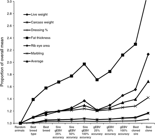
Figure 1 shows the predicted proportional merit for each trait and type of selection, presented as a proportion of the overall mean. The differences between breed types are small for weights and dressing percentage, but, as expected, large for fat thickness. EBV information on individual production animals is probably unlikely to be available. Moreover, assuming low selection pressure for individuals, use of Sire EBV is likely to be of similar value in practice. Notice that superiority for an economic index of traits will generally be lower than the average shown in Fig. 1, because traits are not fully correlated.
|
The results in Fig. 1 give a coarse overview of the impact of different types of genetic information on the management of merit for target traits. The next section addresses the prediction of phenotypes for these traits, as an aid in making more informed management decisions.
Using gEBVs and existing phenotypes to help predict future phenotypes
This section considers how to predict future phenotypes, such as carcass traits, given existing phenotypes, such as weaning weight, plus EBVs or gEBVs. In the simplest case, these are EBVs for the target future traits, but of course they can be EBVs for other related traits. The value of such genetic information for predicting future phenotypes is relevant to initial group formation, but is also relevant to ongoing management decisions, as discussed later, wherever new genetic information is gathered after initial group formation.
The following two approaches are considered:
-
A ‘biological’ approach inspired by mechanistic models of growth and development.
This approach relies on availability of a suitably robust model (see Hirooka (2010), for a review; and Walmsley et al. (2010); http://www.anslab.iastate.edu/Class/AnS426/Old%20files/DECI/Users_Guide.pdf (accessed 8 December 2011) for working models). Means, variances and heritabilities of model parameters (such as rate parameters and mass of different tissue types at maturity) can be estimated, even without sequentially measured target traits (Doeschl-Wilson et al. 2007), such as carcass weight, fat depth and food intake. This was done by searching for means, variances and heritabilities of model parameters that, when used to generate simulated populations, result in maximal correlation between sets of genetic and phenotypic parameters for target traits derived from simulated and real data.
This framework could be used for current purposes; increase the mean value of a target trait, as derived from real data, by a single unit, to reflect an animal or group with an EBV of +1 for that trait, but average EBVs for all other target traits. Then re-analyse for model parameter means following Doeschl-Wilson et al. (2007). The new set of model parameters will change predictions not just for the trait disturbed, but for all traits that the model can predict, including the value for each trait for each day of age. A more complete implementation would consider EBVs for more than one trait, as might be available for individual animals. This approach implicitly infers relationships among all traits that the model can predict, at all ages of expression, giving greater flexibility and applicability for optimising turn-off dates and other aspects of management. However, robustness should be tested, as it is possible that a wide range of changes in model parameters will give a similar fit in explaining an increase of one unit in a target trait, and simple application assumes that the same model applies to both genetic and environmental effects.
A related approach would use covariance functions, in which the (co)variances of target traits are modelled over age (Kirkpatrick et al. 1990). This approach also enables prediction of trait merit at all ages. Neither of these approaches is tested in the present paper.
-
A statistical approach based on selection-index theory.
The method used for this section is given in Appendix 1. Parameters for illustration were taken from Shanks et al. (2001), using the scenario that we predict phenotype for a carcass trait based on phenotypes for weaning weight and/or EBVs (derived from pedigree and/or genetic markers) for the carcass trait. The carcass traits considered were carcass weight and marbling score.
The phenotypes we might use and predict in the production system are generally different from the phenotypes reflected in the parameters we estimate in genetic analyses. The latter are generally corrected for known environmental effects and/or contemporary group membership, whereas in the production system, the phenotypes we use to help make predictions may or may not be corrected, and the phenotypes we want to predict are uncorrected (we eat phenotypes, not corrected phenotypes). The appropriate phenotypic correlation between traits can be bigger or smaller than the estimates we get from analyses that correct for fixed effects and covariables. For example, if ‘good herd background’ has a sufficiently strong positive effect on both weaning weight and carcass weight, the appropriate correlation to use will be higher. Conversely, if compensatory growth gives greater appetite and growth in those from a constraining background, the appropriate correlation to use will probably be lower. Heritabilities for uncorrected phenotypes are lower than for corrected phenotypes, and this generally lowers the value of EBV information. Ideally, we can estimate appropriate parameters within the setting of the production environment. For the current illustration, parameters are from an analysis that corrects for contemporary group effects.
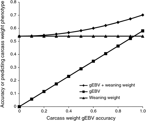
Table 2 shows that, for the parameters assumed, weaning weight is a better predictor of carcass weight than is carcass weight EBV, due to the high phenotypic correlation between these traits. However, combining both sources of information gives a good improvement of prediction accuracy (0.62 v. 0.54).

|
In contrast, weaning weight is a very poor predictor of marbling phenotype, and it adds essentially no power to marbling EBV as a predictor.
Figure 2 shows the effect of EBV accuracy on accuracy of predicting carcass weight. We need very high EBV accuracy to give better predictions than we get from weaning weight. However, combining the two sources of information could be useful, if costs and logistics of accessing EBVs are sufficiently low.
|
For animals whose EBV is derived from their sire’s EBV alone, accuracy will be lower, for example 0.35 for sire EBV accuracy of 0.7. Referring to Fig. 2, this low level of accuracy for carcass weight EBV adds little power to the prediction based on weaning weight phenotype alone (0.56 v. 0.54). This is most relevant to a supply chain with good signals. For example, a feedlotter might prefer high carcass weight EBV animals to high weaning weight animals if she/he pays for young stock on the basis of bodyweight.
Pooling DNA to help predict future phenotypes
The costs of genotyping individual animals to help predict future phenotypes and optimal management regimes is likely to be too high for many scenarios. Genotyping costs can be reduced substantially by using pooling of tissue or extracted DNA derived from many individuals, followed by quantitative genotyping to estimate the frequency of each genetic-marker allele in the pooled sample. The number of genotypings required was reduced from 80 000 to 180, in a hypothetical scenario that infers family mean genetic merit, having individually genotyped the parents of these families (Kinghorn et al. 2010a ).
For current purposes, we are unlikely to have genotypes on parents. However, there is likely to be information on breed mean allele frequencies, such that we can diagnose average breed content of a cohort (Pritchard et al. 2000). Moreover, if we have an appropriate genomic prediction equation, we can use this to help predict the future mean phenotype of the cohort, given a certain management regime. Mean phenotypes will be predicted more accurately than individual phenotypes, and loss of individual information may not be a handicap wherever cohorts cannot be split. To be appropriate, the genomic prediction equation should be relevant to the breed(s) in the cohort pooled, and derived from an appropriately related population(s). The value of such an approach increases if the cohort is more consistent, with less genetic variation among its members, and more variation between cohorts.
Use of crossbreeding to help manage trait merit
The final commercial product in most animal supply chains is based on crossbred animals, with production and cost benefits primarily due to heterosis and breed complementarity. How might genomics play a role in better exploiting crossbreeding? The decision point of relevance is at mating time, somewhat early in the production system. Diagnosis of average breed content, as noted above, could be carried out on unpedigreed herd females, with results being used to form cohorts with choice of breeding males to optimise predicted production efficiency. Of potential future application is the use of genomic information to target increased heterosis expression in crossbred animals in the productions system (Kinghorn et al. 2010b , 2011; Zeng et al. 2011).
Use of genetic information to help manage trait variation
Breed means in T3C were used to calculate variance due to breed type (British and European) and variance due to breed within breed type, under the assumption that the least-squares means in T3C were estimated without error.
Mean squares in T2W were used to give approximate estimates of variance components for the effects listed in that table, under assumptions of orthogonality and balance of design. This effectively treats each effect as if it were fitted alone in a one-way analysis of variance, with expected mean square equalling σerror 2 + nσeffect 2, where n is the number of observations per class.
Breed effects in T2W were not used, because these were taken from T3C, which gives a good split of British and European breed types. Sire effects from T2W were used where appropriate, with residual genetic effects represented in the mean square for error (MSE). Residual genetic and environmental effects coexist in all groupings considered. Thus, there is no need to partition the MSE, with the exception that some components of genetic variation are subtracted from the MSE as noted in Table 3. Identifiable non-genetic components of variance were those due to dam age and weaning age, leaving out year of birth and days on feed, as noted earlier.

|
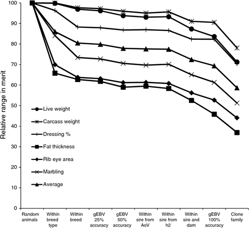
Strategy for grouping on gEBV. Constructing groups based on gEBVs can asymptotically lead to groups within which there is no additive genetic variation, given full accuracy of gEBVs. However, this is not possible in practice, even with full accuracy of gEBVs, because an extremely large population is required to select a group of animals with essentially the same gEBV. This was handled using a simple function of selection intensities for n groups of equal size defined by setting truncation points in a normal distribution, N(0,1). The population variance between the selection intensity points for the n groups, calculated as (sum of squared intensities)/n, is subtracted from the total variance (1) to give the variance within groups, g, as used in Table 3. For n = (1, 2, 3, 4, 5) we get g = (0, 0.64, 0.8, 0.86, 0.9). For example, if we rank animals on gEBV and make five groups of equal size, from the highest to lowest gEBV, the variation in gEBV among and within groups will be 0.9 and 0.1, respectively, of the total gEBV variance.
Figure 3 shows the expected range in trait merit within cohorts genetically grouped according to the methods listed in Table 3, scaled to give a value of 100% for a ‘random’ cohort involving animals of e.g. different breed type, breed and sire. The impact of breed type is critical for fat thickness and rib eye area. Standardising breed within breed type is generally useful, with relatively low impact of grouping on gEBV or sire pedigree within breed. Methods that would add useful consistency are likely to be impractical, i.e. full sib groups, 100% accurate EBV and clone families.
|
Ongoing management decisions: the general case
An integral part of initial management group formation is the plan for management through the segment of the supply chain involved. These things can interact strongly; the best group to form depends on the management plan and the best management plan depends on the group formed. Simultaneous decision making is generally required, even if framed within a broad objective, such as to manage a group of British-type cattle through to a high-marbling slaughter market at a target turn-off date.
The present paper does not consider the full range of management decisions required, but it will attempt to address the nature of decisions to be made and the manner in which genetic and genomic information can be used to make better decisions.
Modelling and optimising performance
An underlying need is the ability to predict the impact of management decisions on future performance of the animals and groups involved. Given knowledge of (1) current state (e.g. genetics, age, current trait measures), (2) forecast conditions (e.g. grass growth, market prices) and (3) planned management (e.g. stocking rate, feedlot entry date, turn-off date), we should be able to predict the outcome in relevant terms (future trait values, variation within cohorts, profit). Such predictions are implicit in all management decisions, but ideally the key factors are predicted explicitly, using a model of animal performance and financial cost–benefit.
To consider the potential impact of genetic and genomic information on such ongoing management decisions, we must first consider the general case, where management is optimised in the face of a wide range of changing conditions and information. The sort of framework required to do this is illustrated by considering the following three examples.
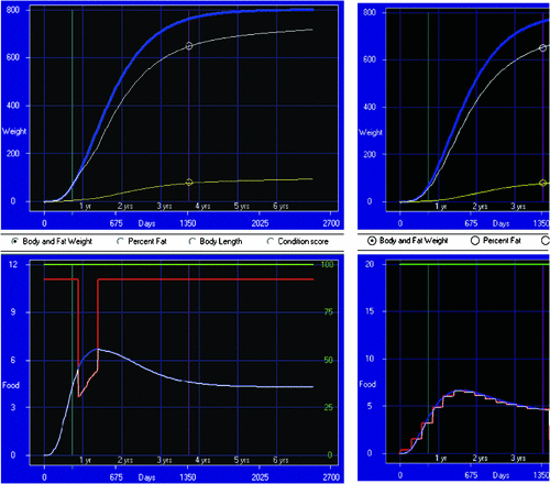
Example 1: feeding and growth. Figure 4 illustrates a simple feeding and growth model, which can predict the impact of level of feed availability and quality (e.g. via stocking rate and feedlot diet formulation) on growth in bodyweight and fat. Given the ability to predict the impact of management, an optimisation algorithm is used to find the management regime that maximises a function of the predicted outcomes. This is illustrated in the right-hand panels of Fig. 4, where target weights and dates have been met, while minimising a function of food consumed and feed costs at different stages.
|
|
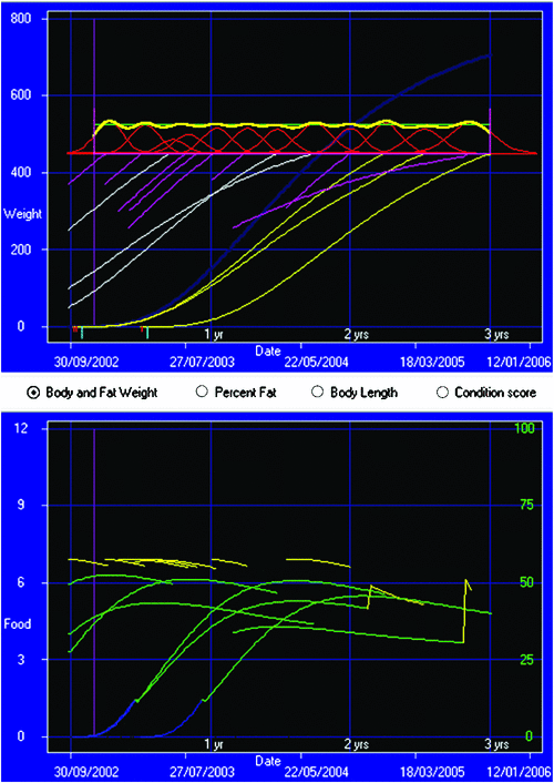
Example 2: consistent supply. Figure 4 is merely illustrative, because it oversimplifies practical and logistical factors involved in real animal production programs. Figure 5 shows one step towards a more realistic scenario, representing a group of producers targeting efficient and consistent supply of beef (Anon 2002). In this case, each feeding or growth line represents a group of animals. The objective function comprises the following:
-
Total growth across lines divided by total food eaten.
-
Penalty for deviation from target weight achieved in each line.
-
Penalty for deviation from target body fat achieved in each line.
-
Penalties for not making target weight within the time window considered.
-
Total cost (value) of pasture eaten across all lines.
-
Total cost of feedlot feed eaten across all lines.
-
Penalty for breaking a declared limit on funds available.
-
Penalties for exceeding target production level on each day of the target period.
-
Penalties for being below target production level on each day of the target period.
-
Penalty for deviation of each future line from its nearest ideal mating date.
Management factors optimised for each line are mating date, levels of feeding when at pasture, as controlled by stocking rate, date of transfer to the feedlot, and date of purchase, number in the line and mean weight for each line to be bought in.
Further flexibility in such a scheme can potentially be achieved by ongoing management of group structure and membership (Kinghorn 1999; Walmsley 2007).
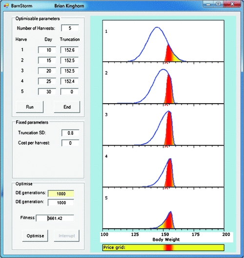
Example 3: targeting a price grid. Figure 6 illustrates a scenario that is more simple, largely because it addresses a narrower question of how do we sequentially harvest stock from a single management cohort to optimise gross returns for a well specified price grid? Briefly, the algorithm used is as follows:
|
-
For the first harvest date (top panel in Fig. 6), animals are grouped into small equal intervals of bodyweight.
-
The truncation weight for the current harvest is used to predict the proportion of animals to be harvested from each interval, and these are removed from the total distribution and evaluated on the price grid.
-
Mean growth and variation in growth to the next harvest date are predicted for each of the intervals, giving a distribution of bodyweight at the next harvest date for animals in the same weight interval at the current harvest date.
-
We now have a distribution of bodyweight at Harvest n for surviving animals out of each interval at Harvest n–1. Sum these distributions to give the overall distribution at Harvest n.
-
Go to step 2, or stop if the last harvest date has been reached.
For simpler illustration, Fig. 6 starts with a normal distribution of bodyweights in the top panel, rather than a real dataset. Note that truncation selection to remove animals for harvesting leaves non-normal distributions of remaining stock. This non-normality reduces as the animals grow. Such effects need to be accounted for to more correctly predict impact of different strategies.
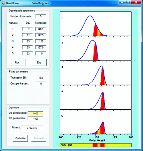
Figure 7 tests a case where two markets favour two different bodyweights, as reflected in the price grid. In this case, the optimal result is to have two harvestings targeting the lighter market and the remaining three harvestings delayed somewhat to target the heavier market.
|
The current example illustrates a simple fixed price grid, with bodyweight as its only dimension, but this can be extended to grids involving multiple traits as well as dynamic grids that change over time as pre-published by the abattoir. Such flexibility is needed for implementation in practice.
As can been seen in Figs 6 and 7, cost per harvesting has been set to zero in these examples, for simplicity. These costs will include cost of labour and any predicted loss in performance due to direct handling, loss of feeding opportunity, and, in some scenarios, behavioural impacts due to reranking in new groups.
Optimisation in practice
The range of possible scenarios for supply chain optimisation is large, with different sets of decision factors to optimise. This means that full optimisation of a supply chain generally requires custom development, and this may be warranted only for relatively large and/or well integrated operations.
It is possible to work separately with component problems, such as the sequential harvesting example above. However, in general, the greater the proportion of supply chain that is simultaneously optimised, the higher the overall benefit. This is because the best action to take at any stage depends not only on past actions, but also on planned future actions. And the best future plan depends on current actions. Making these decisions simultaneously is more efficient.
For the three examples given in this section, optimal outcomes were found using an evolutionary algorithm, as described in Appendix 2.
Ongoing management decisions: the role of genetics
As noted above, genetics is just one of many factors that can have an impact on decisions that have to be made dynamically along the supply chain. Following initial group formation, genetics will usually have a minor role to play in ongoing management decisions. However, certain types of new genetic information could be worth exploiting.
Previous sections have illustrated the use of genetic information to help make sensible decisions on group formation. This included information on breed, EBV and gEBV, and pedigree information. New genetic information that can be generated or otherwise comes to light after initial group formation falls into the following two categories:
-
Information on phenotypic performance of group members themselves, or their relatives. In the latter case, known sires might gain more accurate EBVs, and this would affect EBVs of group members. The value of animals’ own phenotypes recorded during the management process can most usefully be exploited directly, without considering the impact on animal EBV. However, information from outside the group may be of some value.
-
Genomic information gathered on group members.
As for any class of new information, new genetic information has potential to affect decisions at any particular stage in the following three interacting categories:
-
Changing the target product end-point and/or turn-off date.
-
Changing treatment of animals for the balance of time to slaughter.
-
Changing group membership, by splitting or amalgamating groups or parts of groups.
Example: use of a genetic marker for intramuscular fat (IMF)
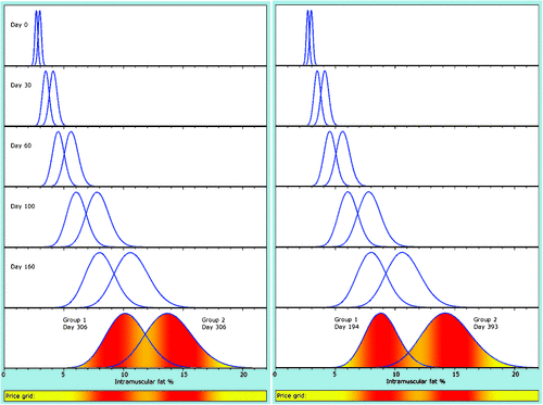
The present example is illustrative rather than evaluative (see Fig. 8), and follows from examples shown in Figs 6 and 7, with a key exception that the trait cannot be measured routinely, such that ongoing grouping for management and marketing purposes cannot be carried out as the trait evolves.
|
The method to generate growth is shown in Appendix 3. Two groups were formed with equal frequency to simply model a binary genetic effect, as might be the case for a dominant genetic marker that is causative for increased IMF. Without knowledge of this genetic marker, and with no direct or indirect measures of IMF, both groups are managed as one, with a single optimal slaughter date, found to be 306 days after feedlot entry (t = 365 + 306 days from birth), as in the left panel of Fig. 8. For simple illustration, optimisation maximises gross return on the price grid illustrated, giving a longer period in the feedlot than would be found under a complete model accommodating factors such as growth in bodyweight and feed costs.
Use of the genetic marker to diagnose group membership (and therefore the potential to achieve high IMF) can be used in several ways, including changing diet and days in the feedlot. Only the latter is considered here. Optimisation results in turn-off at 194 and 393 days post-entry for the low and high groups, respectively. Essentially we have identified the animals with a higher probability of satisfying the high-IMF market, and we feed these animals longer to capitalise on their potential.
Use of the genetic marker gives a 5.9% increase in gross return on the simple price grid assumed, which has a 20% premium for the high-IMF market over the low-IMF market at their respective optima. However, note that this result is merely illustrative. A more reliable result would use a model that accommodates a range of other issues of importance. Moreover, value may accumulate over multiple traits affected by multiple markers.
Genotyping decisions
For the latter example, which optimises time in the feedlot alone, it would be possible to delay genotyping until just before the optimal turn-off date for the short-fed genotype. The longer this delay, the greater the accuracy of any other indirect measure of IMF, e.g. using a scanner, and the greater the opportunity to identify which animals should be genotyped.
Such information is likely to identify some animals that would be placed into one of the two groups with reasonable confidence – and that their destination would not be changed whatever genotyping result were to arise. Thus, only the remaining animals that are liable to change groups should be genotyped. This is ‘genotyping at the edges’ of decision thresholds, and it immediately reduces the number of animals to be genotyped. Moreover, wherever the predicted financial consequence of placing a specific individual in the wrong group is less than the cost of genotyping, then that individual should probably not be genotyped. A more complete treatment of this issue would consider the probability that, without genotyping, the animal is placed in the wrong group. Ultimately, a portfolio approach is required, as group membership influences the optimal management of that group.
Discussion
The present paper does not address the use of breeding programs to enhance livestock production through ongoing genetic improvement. It only considers the use of genetic information to help decide on choice and management of animals to optimise profit, welfare and other impacts in the production system.
Knowledge of breed and seed-stock source has long been used to help manage livestock production, based largely on practitioner experience and trial results. However, proper use of estimates of breeding value, derived using pedigree or genetic markers or both, requires a more solid foundation, based on power to predict future phenotypes using current animal status and future treatment.
Note that we aim to predict phenotypes rather than genetic merit (we eat phenotypes, not genes), and genetic information generally constitutes extra information used to increase accuracy of phenotypic prediction. This means that, in most cases, the framework for using genetic information can function without it. That is why the present paper has placed some emphasis on systems to optimise management in the absence of detailed genetic information.
The present paper has outlined some approaches to integrating genetic information into management decision processes. The diversity of applications in our livestock industries is such that many different approaches are likely to evolve. This contrasts with the use of genetic information in breeding programs, where the goal is comparatively simple.
The work in the present paper is not sufficient to judge the value of genetics to improving livestock production. However, it seems clear that the true value requires information on sizeable genetic effects, for valuable traits that are both quite highly heritable and relatively independent from known phenotypes, and at appropriate cost.
Acknowledgements
The author thanks Brad Walmsley, Scott Newman, Ainsley Archer, Pieter Knap and Andrea Doeschl-Wilson for discussion, and reviewers for useful comments.
References
Anon (2002) Total resource management. In ‘Annual report 2001/2002’. pp. 41–44. The Cooperative Research Centre for Cattle and Beef Quality. Available at http://www-personal.une.edu.au/~bkinghor/TRM%20Annual%20Report%2002.doc [Verified 8 December 2011]Cundiff LV, Wheeler TL, Gregory KE, Shackelford SD, Koohmaraie M, Thallman RM, Snowder GD, Van Vleck LD (2004) Preliminary results from cycle VII of the cattle germplasm evaluation program at the Roman L Hruska US Meat Animal Research Center. Germplasm Evaluation Program Progress Report No. 22. USDA–ARS, Clay Center, NE. Available at http://www.ars.usda.gov/SP2UserFiles/Place/54380000/GPE/GPE22.pdf [Verified 8 December 2011]
Doeschl-Wilson AB, Knap PW, Kinghorn BP, van der Steen H (2007) Using mechanistic animal growth models to estimate genetic parameters of biological traits. Animal 1, 489–499.
| Using mechanistic animal growth models to estimate genetic parameters of biological traits.Crossref | GoogleScholarGoogle Scholar |
Goddard ME (2012) Uses of genomics in livestock agriculture. Animal Production Science 52, 73–77.
| Uses of genomics in livestock agriculture.Crossref | GoogleScholarGoogle Scholar |
Hirooka H (2010) Systems approaches to beef cattle production systemsusing modeling and simulation. Animal Science Journal 81, 411–424.
| Systems approaches to beef cattle production systemsusing modeling and simulation.Crossref | GoogleScholarGoogle Scholar |
Kinghorn BP (1999) Total resource management: tactical optimisation of vertically integrated animal production systems. In ‘The application of artificial intelligence, optimisation and Bayesian methods in agriculture’. (Eds HA Abbass, M Towsey) pp. 95–100. (Queensland University of Technology: Brisbane)
Kinghorn BP (2000) Chapter 18: animal production and breeding systems to exploit cloning technology. In ‘Animal breeding – use of new technologies’. (Eds BP Kinghorn, JHJ Van der Werf, M Ryan) pp. 237–245. (The Post Graduate Foundation in Veterinarian Science of the University of Sydney: Sydney)
Kinghorn BP (2008a) Chapter 4: differential evolution. In ‘Application of evolutionary algorithms to solve complex problems in quantitative genetics and bioinformatics’. (Eds C Condro, BP Kinghorn) pp. 33–37. (Centre for Genetic Improvement of Livestock, University of Guelph: Guelph, Canada). Available at http://www-personal.une.edu.au/~bkinghor/Evolutionary_Algorithms_CGIL2008.pdf [Verified 8 December 2011]
Kinghorn BP (2008b) Chapter 6: introduction to problem representation. In ‘Application of evolutionary algorithms to solve complex problems in quantitative genetics and bioinformatics’. (Eds C Condro, BP Kinghorn) pp. 47–54. (Centre for Genetic Improvement of Livestock, University of Guelph: Guelph, Canada). Available at http://www-personal.une.edu.au/~bkinghor/Evolutionary_Algorithms_CGIL2008.pdf [Verified 8 December 2011]
Kinghorn BP (2008c) Chapter 7: managing constraints. In ‘Application of evolutionary algorithms to solve complex problems in quantitative genetics and bioinformatics’. (Eds C Condro, BP Kinghorn) pp. 55–58. (Centre for Genetic Improvement of Livestock, University of Guelph: Guelph, Canada). Available at http://www-personal.une.edu.au/~bkinghor/Evolutionary_Algorithms_CGIL2008.pdf [Verified 8 December 2011]
Kinghorn BP, Bastiaansen JWM, Ciobanu DC, van der Steen HAM (2010a) Quantitative genotyping to estimate genetic contributions to pooled tissue samples and genetic merit of the contributing entities. Acta Agriculture Scandinavica Section Acta 60, 3–12.
Kinghorn BP, Hickey JM, van der Werf JHJ (2010b) Reciprocal recurrent genomic selection for total genetic merit in crossbred individuals. Paper 0036. In ‘Proceedings of the 9th world congress on genetics applied to livestock production, 1–6 August 2010, Leipzig, Germany’. (Ed. Gesellschaft für Tierzuchtwissenschaften e. V.)
Kinghorn BP, Hickey JM, van der Werf JHJ (2011) Long-range phasing and use of crossbred data in genomic selection. In ‘Proceedings of the 7th European symposium on poultry genetics, Peebles, Scotland’, 5–7 October 2011. pp. 7–9. Available at http://www.roslin.ed.ac.uk/7espg/assets/7espg-edited-proceedings.pdf [Verified 4 January 2012]
Kirkpatrick M, Lofsvold D, Bulmer M (1990) Analysis of the inheritance, selection and evolution of growth trajectories. Genetics 124, 979–993.
Pritchard JK, Stephens M, Donnelly P (2000) Inference of population structure using multilocus genotype data. Genetics 155, 945–959.
Pugh AK, McIntyre BL, Tudor G, Pethick DW (2005) Understanding the effect of gender and age on the pattern of fat deposition in cattle. In ‘Indicators of milk and beef quality’. EAAP publication no.112. (Eds JF Hocquette, S Gigli) pp. 405–408. (Wageningen Academic Publishers: Wageningen, The Netherlands)
Shanks BC, Tess MW, Kress DD, Cunningham BE (2001) Genetic evaluation of carcass traits in Simmental-sired cattle at different slaughter end points. Journal of Animal Science 79, 595–604. Available at http://jas.fass.org/cgi/reprint/79/3/595.pdf [Verified 4 January 2012]
Storn R, Price K (1997) Differential evolution – a simple and efficient heuristic for global optimization over continuous spaces. Journal of Global Optimization 11, 341–359.
| Differential evolution – a simple and efficient heuristic for global optimization over continuous spaces.Crossref | GoogleScholarGoogle Scholar |
Walmsley BJ (2007) Modelling of growth and development for optimising beef cattle production systems. PhD Thesis, University of New England, Armidale, NSW.
Walmsley BJ, Oddy VH, McPhee MJ, Mayer DG, McKiernan WA (2010) BeefSpecs a tool for the future: on-farm drafting and optimising feedlot profitability. AFBM Journal 7, 29–35. Available at http://www.beefcrc.com.au/BeefSpecs [Verified 8 December 2011]
Wheeler TL, Cundiff LV, Shackelford SD, Koohmaraie M (2004) Characterization of biological types of cattle (Cycle VI): carcass, yield,and longissimus palatability traits. Journal of Animal Science 82, 1177–1189. Available at http://www.ars.usda.gov/SP2UserFiles/Place/54380530/2004041177.pdf [Verified 4 January 2012]
Zeng J, Toosi A, Fernando RL, Dekkers JCM, Garrick DJ (2011) Genomic selection of purebred animals for crossbred performance under dominance. In ‘Proceedings of the 7th European symposium on poultry genetics, Peebles, Scotland’, 5–7 October 2011. pp. 83–84. Available at http://www.roslin.ed.ac.uk/7espg/assets/7espg-edited-proceedings.pdf [Verified 4 January 2012]
Appendix 1. Method to predict future phenotypes from existing phenotypes and EBVs
The objective is to predict phenotype for one or more traits, and the criteria are phenotypes for different traits and/or EBVs for any traits (as derived using pedigree, genetic markers or both). To illustrate the method, the following example is used:
-
criteria: phenotype for Trait 1 (p 1) and EBV for Trait 2 (
 );
); -
objective: phenotype for Trait 2 (p 2).
Our estimate of p
2 for an individual is  , where b is a column vector of index weights and cis a column vector of criteria for the individual concerned.
b = CC –1 × CO, where CC is the criterion × criterion (co)variance matrix and CO is the criterion × objective (co)variance matrix. In our example:


where  is the accuracy of
  , and r
A
1,2
(r
P
1,2
) is the genetic (phenotypic) correlation between Traits 1 and 2.
This assumes that p
1 is not involved in the calculation of  (otherwise non-genetic covariance should be accommodated). By definition, p
2 is not involved in the calculation of
  .
.
Accuracy of predicting the objective, given the criteria, as reported in the text, is  .
.
Predicted phenotypes are typically neutral with respect to identifiable environmental effects, other than those included in the phenotypes available as criteria. Better predictions can be made given knowledge of these factors, such as days on feed and pasture quality. A biologically inspired model of growth may do this more effectively than does a linear statistical model.
Given the use of parameters derived from analyses that account for known environmental effects, the accuracies as predicted in this appendix tend to be optimistic if variation due to such effects influences the objective phenotypes, and they are not accounted for following initial prediction.
Appendix 2. Optimisation methods
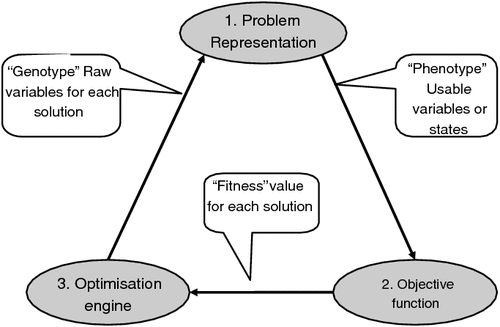
For the examples given in the text, optimal outcomes were found using an evolutionary algorithm. This process has the following three key components (Fig. A1) used iteratively over ‘generations’ to derive the optimal solution:
-
A problem representation component that uses a vector of numbers (analogous to a multilocus genotype) and translates these numbers to a representation of a solution (analogous to a phenotype), which in this case is a full management regime.
-
An objective function component that evaluates each ‘phenotype’ to calculate its fitness (analogous to selective advantage). In our case, this is a single figure that represents utility (profitability or similar), as calculated by a predictive model.
-
An optimisation component that uses the fitness value for each of the ‘genotypes’ that it has produced to help select, mutate and recombine existing ‘genotypes’, to provide new candidate ‘genotypes’.
A key advantage of this approach is that the optimisation engine is highly disjointed from the problem itself. It does not ‘know’ or ‘understand’ the problem; it simply delivers candidate solutions as sets of parameters, in a raw form, and receives feedback on the value of each of these solutions. This means that the problem itself can become increasingly complex, without the need to increase the complexity of the optimisation machinery.
Given this disjointed nature of the optimisation engine, the current paper does not include a detailed description of the optimisation engine that it uses to generate results. It is based on differential evolution (DE, Storn and Price 1997), with adaptations described by Kinghorn (2008a , 2008b , 2008c ).
Appendix 3. Method to generate Fig. 8
Data on intramuscular fat (IMF) from Pugh et al. (2005) as supplied by D. W. Pethick (pers. comm.) were fitted to days-on-feed, using a powered exponential decay function, assuming a mean IMF at birth of 2% and a feedlot entry age of 365 days. The functional form was

where t is time in days, 0 is birth, IMF ∞ is asymptotic IMF at maturity, k is a time scaling factor and p is the power. The fitted parameters were IMF ∞ = 12.78, k = 0.01203 and p = 206.74, giving R 2 = 0.9974
Growth in IMF was modelled as follows:
At t = 0, a frequency distribution of IMF was generated with a mean of 2 and s.d. of 0.1. For each small interval, growth to the next time-point (feedlot entry at t = 365 days) was predicted using Eqn A1, with IMF ∞, k and p as fitted, and the contribution from this interval at t = 0 was spread among the IMF intervals at t = 365, using a normal distribution with a coefficient of variation of growth of 0.1. These distributions at t = 365 were summed over the contributing t = 0 intervals, to give the overall frequency distribution for t = 365.
The treatment for growth to later time-points differs as follows: for each interval at t – 1, solve for IMF ∞ using Eqn A1 with k and p as fitted and IMF 0 = 2. Use this value of IMF ∞ to predict growth from t–1 to t for that small interval, and spread this contribution among the IMF intervals at time t using a coefficient of variation of growth of 0.1.
This treatment generally leads to slightly right-skewed distributions at later ages, with animals with a higher IMF at a given time being predicted to have a higher IMF at maturity and higher growth in IMF.
A binary genetic effect was simulated by generating two groups of animals of equal frequency. The high group was generated with a 10% higher value for both IMF 0 and the initial IMF ∞ used to generate the population at t = 0. These increased values result in more than 10% increase in IMF due to accumulation of effects.

|

|


