

Economic risk analysis of different livestock management systems
J. F. Scott A D , O. J. Cacho B and J. M. Scott CA NSW Trade and Investment, 4 Marsden Park Road, Tamworth, NSW 2340, Australia.
B University of New England, School of Economics, Armidale, NSW 2351, Australia.
C University of New England, School of Environmental and Rural Science, Armidale, NSW 2351, Australia.
D Corresponding author. Email: fiona.scott@industry.nsw.gov.au
Animal Production Science 53(8) 788-795 https://doi.org/10.1071/AN11249
Submitted: 20 October 2011 Accepted: 20 March 2012 Published: 10 July 2013
Journal Compilation © CSIRO Publishing 2013 Open Access CC BY-NC-ND
Abstract
The Cicerone farmlet experiment, conducted on the Northern Tablelands of New South Wales, Australia, explored aspects of profitability and sustainability under three different whole-farmlet management regimes. The 5-year period over which the treatments were measured occurred over a period of generally below-average rainfall, hence responses to management treatments were limited. A modelling approach was used to estimate profitability over a longer period representing the variable climate of the region. A stochastic discounted cash flow model was developed to estimate economic returns of two of the Cicerone management system treatments scaled up from the farmlet scale (53 ha) to the size of a typical commercial farm in the region (920 ha) over a 20-year period. Several scenarios were used to estimate the commercial-scale returns under different rates of pasture improvement and stocking rates. Over the long-term, Farm A was found to be more profitable but also more risky (in terms of variation around the mean of cumulative discounted cash flow) than the ‘typical’ Farm B management system. If livestock managers choose to adopt a pasture improvement strategy based on renovating pastures and increasing soil fertility, they are more likely to achieve higher net worth with more moderate rates of pasture improvement than those explored on Farm A where a high rate of pasture improvement had been implemented in order to quickly differentiate treatments.
Introduction
The climate of the Northern Tablelands of New South Wales, Australia, where the Cicerone livestock management systems were compared on farmlets, is quite variable, and the climate experienced during the experimental period was not representative of the climatic conditions expected over the long-term (Behrendt et al. 2013b).
Pannell et al. (2000) concluded that ‘getting the big decisions right’ is the key for farmers to achieve their objectives of staying in farming and increasing their wealth. By ‘big decisions’ they meant land purchases, machinery investment and resource improvements; in this context, investment in sown pastures would constitute a resource improvement. Therefore, it is appropriate to compare the risk profiles of the Cicerone management system treatments at a commercial scale. The difference between the profitability of the three different management systems was compared at both the farmlet (53 ha) and typical whole-farm (920 ha) commercial scale in an earlier, related paper by Scott et al. (2013a).
Behrendt et al. (2006) observed that direct comparison of the Farm A production and financial performance results against those of Farm B may not provide a reasonable comparison. This was because the high rate of pasture improvement, which was necessary to differentiate the farmlet treatments quickly (Scott et al. 2013b), was shown to be well below the risk-efficient frontier. In risk analysis, the risk-efficient frontier demonstrates the trade-offs between profit and risk and shows a range of stochastically-efficient profit-risk combinations which producers can choose from, depending on their personal level of risk aversion (Hardaker et al. 2004).
Initially, Farm A had high inputs of sown pastures and fertilisers (aiming to improve pastures on 100% of the farmlet in 5 years) and used flexible rotational grazing in an eight-paddock system. Farm B had a similar grazing pattern and number of paddocks to Farm A but maintained moderate levels of soil fertility with little pasture renovation. Analysis by Behrendt et al. (2006) found that reducing the pasture improvement rate for Farm A from 20% of the farm area per year to 4% (while keeping the ultimate goal of 100% of the farmlet to be sown to pasture) would move the farmlet to the risk-efficient frontier and allow a fairer comparison between the two. As a result of these findings, the question arose of how the profitability and risk of this lower rate of pasture improvement on Farm A would compare to Farm B; this question is addressed by this paper.
The Cicerone Project trial period occurred during an extended period of below-median rainfall (Behrendt et al. 2013b), so the various data measured could not be used alone to construct the stochastic model. A simulation model was required to estimate animal production with Cicerone farmlet management strategies under a full range of climatic conditions. The impact of production risk over time (which varies with climate) was estimated using stochastic simulation analysis which enabled assessment of the variability of possible results. Four different scenarios were used to estimate the commercial-scale cash flow returns under different rates of pasture improvement and the resulting differing stocking rates. The Farm C management strategy, which implemented intensive rotational grazing on 37 paddocks, was unable to be evaluated because at the time, the GrassGro model could only represent up to 10 paddocks in a grazing system (K. Behrendt, pers. comm.).
To compare alternative investments, discounted cash flow budgets were used to adjust benefits and costs received over several years to the same value (usually present value) in order to determine which alternative would be the most profitable (Malcolm et al. 2005). Once the flows of future income and costs were expressed in equivalent dollar values, the total costs were subtracted from the total benefits to give the net present values (NPV) of the investment.
Methods and data sources
Recent examples of deterministic modelling using the discounted cash flow approach include Scott et al. (2000), Barlow et al. (2003) and Trapnell et al. (2006). Scott et al. (2000) used a comparative 15-year cash flow for different levels of inputs (fertiliser, herbicides and feed supplements), while Barlow et al. (2003) used net cash flow analysis for beef, self-replacing Merino and prime lamb enterprises over a 10-year period. Trapnell et al. (2006) analysed the economic and financial implications at the paddock level of different grazing systems in Victoria over a 13-year time period. The results from the latter study indicated that changing from low input pasture with low stocking rates to high stocking rates and fertiliser addition was a profitable option.
Behrendt et al. (2006) used results from the Cicerone project from 2000 to 2005 to calibrate the decision support tool GrassGro (Moore et al. 1997) to represent two pasture types. The assumption made in the model was that a Merino ewe-based wool enterprise was the only enterprise on the farm. The pasture types were ‘sown’ (predominantly introduced species as on Farm A) and ‘degraded’ (predominantly warm-season native and annual grasses as on Farm B) (Behrendt et al. 2006). Using the GrassGro simulation model, climatic data for Armidale from 1959 to 2003 were used to estimate wool and sheep meat production based on a self-replacing Merino flock (Behrendt et al. 2006, 2013a). Five different pasture types were modelled; a degraded pasture with a stocking rate of 3.8 ewes/ha and a sown pasture with stocking rates of 3.8, 6, 8 and 10 ewes/ha. The 3.8 ewe/ha stocking rate was equivalent to the 8.5 dry sheep equivalent (DSE)/ha target stocking rate for Farm B, with the 6 ewe (11.9 DSE)/ha stocking rate representing Farm A (described in more detail below in Scenarios 1 and 2).
The stochastic variables estimated using the GrassGro simulation model by Behrendt et al. (2006) were annual livestock sales and purchases (number of and mean bodyweight at sale for wethers, ewe lambs and cast-for-age stock sold, number of rams purchased), wool production (number of ewes and weaners shorn, wool production per head, mean wool fibre diameter) and supplementary feed required for maintenance. The annual values of these variables were used as the basis for input distributions in the models by using BestFit (Palisade 2000) to choose the distribution that yielded the ‘best fit’ representation for each parameter under each stocking rate (Table 1).

|
The Chi-square test statistic was used to determine which distributions were the best fit for the annual values for each variable. In some cases, the distributions differed between pasture types due to the different responses of the parameters in the model under the different stocking rate scenarios over the time period modelled. Each distribution was truncated when necessary to prevent negative values being used in the stochastic scenario models, such as number of stock sold.
Dependence between random variables was estimated by generating correlation matrices using the Excel add-in software, @RISK (Palisade 2000). These correlation matrices were then used in the stochastic analysis. This allowed for correlation between inputs (such as supplementary feed) and outputs (such as wool diameter, wool yield and liveweight) to be included in the stochastic simulations.
Discounted cash flow spreadsheet models were constructed in Microsoft Excel for each scenario analysed. Data for each scenario included annual sheep production figures (numbers sold, wool produced) as well as product prices, variable costs per head and overhead costs. The input distributions were then used in each stochastic simulation cash flow model to derive NPV of cash flow outcomes at the commercial scale over a 20-year time period using @RISK. The 20-year time period allowed for pasture improvement levels in one of the Farm A scenarios being analysed to reach 100%. The Latin Hypercube sampling method was used in the scenario models since this forces the sampling to include outlying events more frequently, and therefore it more accurately estimates the low probability outcomes compared with Monte Carlo sampling (Palisade 2000; Hardaker et al. 2004). In order to establish the variability of profitability, dependence between random variables was estimated by generating correlation matrices using @RISK. These correlation matrices in turn allowed generation of jointly-distributed series of random values. This allowed for correlation between inputs (such as supplementary feed) and outputs (such as wool diameter, wool yield and liveweight) to be assessed in the stochastic simulations.
Stochastic simulation allowed the generation of cumulative distributions for each scenario for NPV after tax and trends in the probability distributions for profit over the analysis period.
Cost assumptions
Several background assumptions were made regarding key input as well as output prices. Maintenance fertiliser was assumed to be 1.1 kg of phosphorus per DSE per year (Guppy et al. 2013), applied as single superphosphate since it accounts for the majority of fertiliser applied to pastures on the Northern Tablelands. Based on calculations for the last year that costs and income were available (2005), a bulk price of $280 per tonne (ex-GST) for single superphosphate was used.
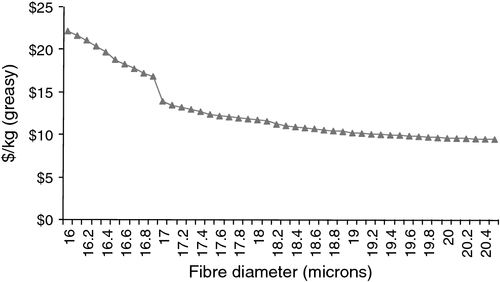
The discounted cash flow analysis was focussed on production risk, so wool price was only varied between wool fibre diameter grades. The GrassGro model output did not provide staple strength estimates so a single price grid (Fig. 1) for wool staple strength between 35 and 50 N/ktex was used, based on average greasy wool price grids from 2002, 2003 and 2004. Most wool produced from the Cicerone farmlets fell within this staple strength range (Cottle et al. 2013). GrassGro model output was also in terms of clean wool cut per head, this was converted to greasy fleece weight using a conversion factor of 0.69 (NSW DPI 2005). Other price assumptions used were $640 per head for replacement rams, $2.00/kg dressed (carcass) weight for wether and ewes sold and $1.00/kg dressed weight for cast-for-age stock sold. Dressed weight was assumed to be 45% of liveweight.
Variable costs per head were based on the recorded values from the Cicerone farmlet experiment or New South Wales Department of Primary Industries gross margin budget costs where unit costs were too high due to the small scale of the farmlets. Costs used included $2.50 per head (for ewes) and $0.51 per head (for lambs) for vaccine and drenches, $1.45 per head for marking and mulesing of lambs, $5.45 per head for shearing, $51.39 per bale (testing, commission, wool packs), wool tax was 2% plus $1.50 per head livestock selling costs and 4.5% commission on sales. These costs were linked to annual livestock numbers and wool production, which varied for each iteration of the stochastic simulation.
Supplementary feed was the only key input that was directly derived from probability distributions using GrassGro output. Feed mix assumptions were that sheep were fed with a 50% cottonseed meal and 50% lupin feed mix (Behrendt et al. 2006) to maintain liveweight when ewe fat score fell below 2.5 and when weaner fat score fell below 2 (K. Behrendt, pers. comm.). Using long-term average prices, the cost of feed was estimated at $300 per tonne.
Where extra sown pasture was required after 2005–06 in the scenarios analysed, the sowing cost was assumed to be $250/ha. This was the average annual cost per ha for sowing individual paddocks of Farm A and included pre-sowing herbicides, fertiliser and a three-species pasture seed mix (tall fescue and phalaris perennial grasses plus white clover) and contract sowing of $75/ha. While this cost is relatively high, it is justified because the scenarios assume that the sown pasture is replacing a degraded pasture containing red grass, subterranean clover, annual grass (Vulpia spp.) and wallaby grass (Austrodanthonia spp.), which would require treatment with herbicides and additional fertiliser.
Allowance for taxation was included because the tax deductibility of the annual costs of capital investments (such as sown pastures) reduces the real cost of such investments (Malcolm et al. 2005) and is therefore relevant. In the case of sown pastures, the investment is deductible in equal instalments over 10 years (Malcolm et al. 2005; Trapnell et al. 2006). The deductible interest was counted in the deductibles for the after-tax calculations. A marginal tax rate of 25% (Trapnell et al. 2006) was assumed and the deductibility of expenditure on sown pastures allowed for in the discounted cash flow models. Hence the returns to capital were all calculated after tax.
The discounted cash flows were based on an economic analysis which included salvage values for livestock (at market value) and sown pasture at the end of the time period. The salvage value used for sown pasture was 50% of the cost of establishment over the 20-year period (Malcolm et al. 2005). The difference between capital invested and capital recouped at the end of the time period is the depreciation cost over the time period analysed (Malcolm et al. 2005) and allows the calculation of the correct NPV (Trapnell et al. 2006). Barlow et al. (2003) also used net cash flow analysis to evaluate the economic returns for different grazing systems and assumed that a proportion of the initial capital invested in pasture development still existed at the end of the analysis period.
A discount rate of 6.7% (real) was used for each example. The approach of using real terms rather than nominal is favoured due to the difficulty in making predictions about future inflation rates and future trends in the relative prices of inputs and outputs (Sinden and Thampapillai 1995; Malcolm et al. 2005). The interest rate on borrowings and the inflation rate entered in the model parameters were used to calculate the real discount rate, using the following formula:
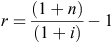
where n is the nominal interest rate and i is the inflation rate.
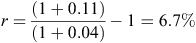
The derived discount rate was calculated using 11% for the interest on borrowings and 4% for inflation, hence:
Scenarios analysed
Different scenarios were used to estimate the commercial-scale returns under different rates of pasture improvement and stocking rates on systems representing high inputs and high stocking rate (Farm A) and moderate inputs with lower target stocking rate (Farm B). These scenarios were:
-
Scenario 1 Farm A: 11.9 DSE/ha.year, 4% re-sowing, first 5 years using Cicerone results
-
Scenario 1 Farm B: 8.5 DSE/ha.year, 2% re-sowing, first 5 years using Cicerone results
-
Scenario 2 Farm A: 11.9 DSE/ha.year, 4% re-sowing, all years using model results
-
Scenario 3 Farm A: 15 DSE/ha.year, 4% re-sowing, all years using model results
These are explained in more detail below.
Scenario 1 for both Farms A and B used the actual Cicerone farmlet income and costs scaled up to a typical, commercial scale (920 ha) for the 5 years 2000–01 to 2004–05, which included both wool and trade cattle enterprises. The actual results for the first 5 years were used in order to give a representation of the expected values of NPV and the risk profile from 2005 to 2006. For the years 2005–06 to 2019–20, GrassGro distributions for the main output and supplementary feed parameters were used. This meant that from 2005 to 2006 onwards, only the production benefits from a wool and sheep meat enterprise were included.
In the case of Farm A, after 2004–05, maintenance fertiliser was applied annually to the pastures but pasture re-sowing was assumed to be required at a rate of 4% of the farm area per year. Given that single superphosphate is 8.8% phosphorus, the maintenance fertiliser amount required for Farm A stocked at a target of 11.9 DSE/ha.year was 149 kg/ha.year of single superphosphate and for Farm B, stocked at a target of 8.5 DSE/ha.year the amount required was 100 kg/ha.year (given that 1.1 kg/ha.year of phosphorus is required for maintenance). The stocking rate of 11.9 DSE/ha was below the Cicerone target stocking rate of 15 DSE/ha, but indications from recent publications have shown that the initial target stocking rate of 15 DSE/ha for Farm A was too high within the 5 dry years experienced, exhibited by a decline in the weight gain of weaners in the final year on Farm A (Hinch et al. 2013). In the case of Farm B, a lower percentage of pasture re-sowing (2% of the farm area) per year was assumed after 2005–06. Maintenance fertiliser was applied annually to the remainder of the farm area. This was consistent with the management strategy for Farm B, which allowed for the maintenance of moderate levels of soil fertility and occasional pasture renovation.
Scenario 2, which applied to Farm A only, was based on a pasture re-sowing rate of 4% per year starting in 2000–01 with a target stocking rate of 11.9 DSE/ha (6 ewes/ha). Income and variable cost figures for all years were generated from GrassGro-derived probability distributions and were based on a wool and sheep meat enterprise.
Scenario 3, which also applied to Farm A only, was based on a pasture improvement rate of 4% per year starting in 2000–01 with a target stocking rate of 15 DSE/ha (8 ewes/ha) identified as risk-efficient by Behrendt et al. (2006). Income and variable cost figures for all years were also generated from GrassGro-derived probability distributions and were based on a wool and sheep meat enterprise. The stocking rate for this scenario was the target rate for Farm A in the Cicerone guidelines (Scott et al. 2013b). The maintenance fertiliser amount required was 185 kg/ha.year of single superphosphate.
Results
The mean NPV, standard deviation of NPV and benefit-cost ratio (BCR) results for the scenarios analysed using stochastic simulation are reported in Table 2. The NPV for Farm A-Scenario 1 (Farm A-S1) was slightly higher than that for Farm B-Scenario 1 (Farm B-S1) due to the higher salvage values at the end of the time period. These higher salvage values were due to a combination of higher livestock numbers and higher capital expenditure on sown pastures for Farm A-S1. The BCR results for Farm A were lower than for Farm B due to higher costs that occurred under the Farm A scenario.

|
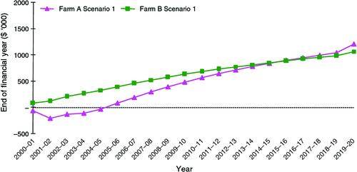
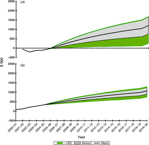
Cumulative discounted cash flows are shown in Fig. 2 for Scenario 1 using mean values from the stochastic simulations. The first 5 years reflect actual Cicerone outcomes at the commercial scale, with years 2005–06 to 2019–20 for a wool enterprise based on the assumptions described above.
|
The NPV for Farm B was lower than for Farm A but the standard deviation was considerably lower indicating Farm B has a lower level of risk in cash flow outcomes. However, as shown in Table 1, most of the variables used in the stochastic scenario models do not have normal distributions. Comparison of the scenario outcomes on the basis of mean against standard deviation is only approximate since the assumption behind mean standard deviation efficiency analysis is that the underlying distributions are normal (Hardaker et al. 2004).
Summary charts of the cumulative discounted cash flows for Scenario 1 on Farms A and B are given in Fig. 3. These charts display change in risk over time for each scenario and the trends in the distribution of cumulative discounted cash flow from year to year. The band (dotted area) shows the range of one standard deviation around the mean. The solid (green) band shows the range between the 5th and 95th percentiles. The smaller bands around the means for the Farm B scenario reflects its lower variability compared with Farm A, also shown by the lower Farm B standard deviation in Table 2.
|
Scenario 2, with a moderate pasture improvement rate (4% per annum), returned a slightly lower NPV after tax than Scenario 3 with a higher standard deviation and a lower BCR (Table 2).
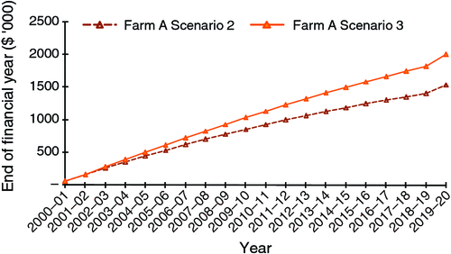
Means of the cumulative discounted cash flows for Farm A, Scenarios 2 and 3, are shown in Fig. 4. Scenario 3 has a higher mean cumulative cash flow due to a higher level of production. This scenario also has a higher cost of maintenance fertiliser, but the same rate of pasture re-sowing as Scenario 2 at 4% of 920 ha, or 37 ha, per year.
|
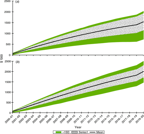
The NPV for Scenario 2 has a lower mean but also has a higher variability (and therefore risk) as measured by standard deviation. Summary charts for the cumulative discounted cash flows for Farm A, Scenarios 2 and 3, are found in Fig. 5. Both have lower variability than Scenario 1 and a much lower probability of negative returns.
|
These findings correspond to those of Behrendt et al. (2006) confirming that Farm A is more profitable but also more risky (in terms of variation around the mean of cumulative discounted cash flow) than the ‘typical’ Farm B management system. The least risky of the Farm A scenarios was Scenario 3, where only 4% of the farm area per year was renovated and a higher stocking rate was maintained.
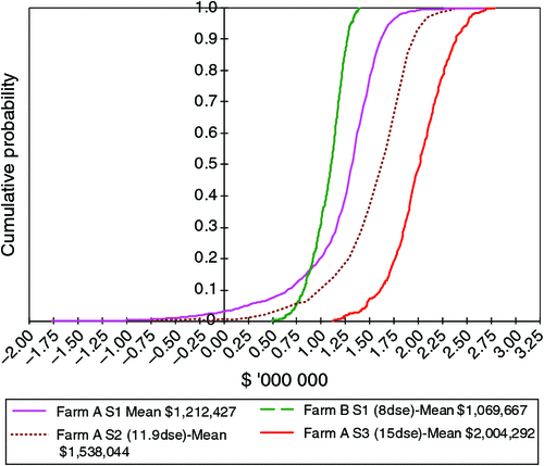
Stochastic dominance
The cumulative probability distributions for each scenario for NPV after tax are shown in Fig. 6. These allow comparisons in terms of the full distribution of outcomes. The rule of first-degree stochastic dominance states that given two alternatives labelled D and E, each with a probability distribution of outcomes x, defined by cumulative distribution functions (CDF), FD(x) and FE(x) respectively, alternative D will dominate alternative E if FD(x) ≤ FE(x) for all crosses (Hardaker et al. 2004). Graphically this means that a CDF of alternative D will lie to the right of that of alternative E.
|
The CDF for NPV of cash flow for Farm A-S1 [FA-S1(x)] crosses that of Farm B-S1 [FB-S1(x)] (Fig. 6) indicating neither dominates the other in terms of first-degree stochastic dominance. For lower values of x, FB-S1(x) is the superior of the two, but for higher values of x, FA-S1(x) is superior. This indicates there is a small probability that Farm A-S1 may be less profitable than the Farm B-S1 over the 20-year time period. FA-S1(x) has the highest standard deviation, indicating it has the highest variability. The difference between them shows the higher potential productivity of the Farm A scenario.
The cumulative probability distributions for NPV after tax for Scenarios 2 and 3 shown in Fig. 6 indicate that Farm A-S3 [15 DSE/ha, FA-S3(x)] dominates Farm A-S2 [11.9 DSE/ha, FA-S2(x)].
Discussion
Using stochastic simulation analysis for Scenario 1, Farm A had a higher NPV after tax than Farm B. This appeared to be mostly due to the higher potential productivity for Farm A and higher salvage values for livestock and sown pasture at the end of the 20-year period. Analysis of the trends in the distribution of cumulative discounted cash flow from year to year for Scenario 1 showed much higher production-driven variability associated with Farm A. These results assumed a low rate of sown pasture on each farm in each year to maintain productivity, without allowance for pasture establishment failure due to dry seasonal conditions. Cumulative probability distributions of NPV for Scenario 1 indicated that there is a small probability (~7%) that Farm A-S1 may be less profitable than the Farm B-S1 over the 20-year time period.
Farm A-S2, with a target stocking rate of 11.9 DSE/ha, returned a slightly lower NPV than Farm A-S3 (target stocking rate 15 DSE/ha). Both had a moderate pasture improvement rate (4% per annum) starting in year 1, with animal production based on a wool enterprise alone. Scenario 3, with a higher stocking rate, had a lower standard deviation of NPV than Scenario 2. At a higher stocking rate, the production potential is higher but so is the amount of supplementary feed that needs to be purchased in dry seasons. This is consistent with the findings of the Cicerone farmlet experiment where the higher stocking rate of Farm A resulted in a higher level of supplementary feeding (Scott et al. 2013b).
A comparison of cumulative probability distributions of the NPV for Farm A Scenarios indicated that Scenario 3 dominated Scenario 2, which in turn dominated Scenario 1. This corresponds to the findings of Behrendt et al. (2006) who observed that Scenario 3 was the risk-efficient option for a Farm A management system, when compared with either a 20% per year pasture improvement rate at 15 DSE/ha (Scenario 1) or a 4% per year pasture improvement rate at 11.9 DSE/ha (Scenario 2). Also, as observed by Behrendt et al. (2006), Farm A can be more profitable but also tends to be more risky (in terms of variation around the mean of cumulative discounted cash flow) than the ‘typical’ Farm B management system.
The scenario analysis for the commercial-scale Farm A has shown that it has the potential to realise good returns; however, there is a higher level of variability of returns associated with the Farm A approach. A commercial-scale Farm B performed the best in terms of whole-farm profitability to the end of June 2005, but its profitability may decline over time due to the decline in digestible pasture species that was documented over the last 5 years of the experiment by Shakhane et al. (2013). This farm has much less ability to take advantage of ‘good’ seasons, due to lower fertiliser and sown pasture inputs, a lower stocking rate and lower legume content, limiting the ability of pastures and subsequent animal production to respond to higher rainfall seasons. Nevertheless, this is a lower risk system in terms of variability and it is less intense in terms of management and capital inputs compared with a Farm A system.
It could be said that sustainability depends on maintaining natural resources (The World Bank 2005) while being able to prevent excessive losses in poor seasons and also being able to take advantage of good seasons, particularly in the establishment period of sown pastures. But often, as in the case of Farm A, the investment in altering the production system to take advantage of good seasons, carries with it increased risk of higher losses in poor seasons. Malcolm et al. (2005) stated that ‘risk and uncertainty make it possible to earn good profits’. However, it is a ‘tricky balancing act’ to have sufficient exposure to risk to achieve farm business goals, while without being at risk of going bankrupt (Malcolm et al. 2005). Whether Farm A would be a successful investment, would depend on the individual business structure and financing (i.e. debt levels required, thus influencing exposure to financial risk), the skill level of the grazier and subsequent seasonal outcomes and impacts on growth, profit and cash flow.
Acknowledgements
The authors wish to thank the members, team and Board of The Cicerone Project Inc. for making data available and, in particular, the contribution of Caroline Gaden (Cicerone Project Executive Officer), Justin Hoad (Cicerone Project Farm Manager), Karl Behrendt (GrassGro modelling data) as well as Dion Gallagher and Colin Lord of the Relational Database Unit, University of New England. The Cicerone Project was supported by Australian Wool Innovation.
References
Barlow R, Ellis NJS, Mason WK (2003) A practical framework to evaluate and report combined natural resource and production outcomes of agricultural research to livestock producers. Australian Journal of Experimental Agriculture 43, 745–754.| A practical framework to evaluate and report combined natural resource and production outcomes of agricultural research to livestock producers.Crossref | GoogleScholarGoogle Scholar |
Behrendt K, Cacho O, Scott JM, Jones R (2006) Methodology for assessing optimal rates of pasture improvement in the high rainfall temperate pasture zone. Australian Journal of Experimental Agriculture 46, 845–849.
| Methodology for assessing optimal rates of pasture improvement in the high rainfall temperate pasture zone.Crossref | GoogleScholarGoogle Scholar |
Behrendt K, Cacho O, Scott JM, Jones R (2013a) Optimising pasture and grazing management decisions on the Cicerone Project farmlets over variable time horizons. Animal Production Science 53, 796–805.
| Optimising pasture and grazing management decisions on the Cicerone Project farmlets over variable time horizons.Crossref | GoogleScholarGoogle Scholar |
Behrendt K, Scott JM, Mackay DF, Murison R (2013b) Comparing the climate experienced during the Cicerone farmlet experiment against the climatic record. Animal Production Science 53, 658–669.
| Comparing the climate experienced during the Cicerone farmlet experiment against the climatic record.Crossref | GoogleScholarGoogle Scholar |
Cottle D, Gaden CA, Hoad J, Lance D, Smith J, Scott JM (2013) The effects of pasture inputs and intensive rotational grazing on superfine wool production, quality and income. Animal Production Science 53, 750–764.
| The effects of pasture inputs and intensive rotational grazing on superfine wool production, quality and income.Crossref | GoogleScholarGoogle Scholar |
Guppy CN, Edwards C, Blair GJ, Scott JM (2013) Whole-farm management of soil nutrients drives productive grazing systems: the Cicerone farmlet experiment confirms earlier research. Animal Production Science 53, 649–657.
| Whole-farm management of soil nutrients drives productive grazing systems: the Cicerone farmlet experiment confirms earlier research.Crossref | GoogleScholarGoogle Scholar |
Hardaker JB, Huirne RBM, Anderson JR (2004) ‘Coping with risk in agriculture.’ (CAB International: Wallingford, UK)
Hinch GN, Hoad J, Lollback M, Hatcher S, Marchant R, Colvin A, Scott JM, Mackay D (2013) Livestock weights in response to three whole-farmlet management systems. Animal Production Science 53, 727–739.
| Livestock weights in response to three whole-farmlet management systems.Crossref | GoogleScholarGoogle Scholar |
Lance D (2004) Evaluation of the impact of pasture and grazing management on sheep and wool quality and economic returns. Bachelor of Rural Science 4th-year thesis, University of New England, Armidale, Australia.
Malcolm B, Makeham JP, Wright V (2005) ‘The farming game: agricultural management and marketing.’ (Cambridge University Press: Melbourne)
Moore AD, Donnelly JR, Freer M (1997) GRAZPLAN: decision support systems for Australian grazing enterprises III. Pasture growth and soil moisture models and GrassGro DSS. Agricultural Systems 55, 535–582.
| GRAZPLAN: decision support systems for Australian grazing enterprises III. Pasture growth and soil moisture models and GrassGro DSS.Crossref | GoogleScholarGoogle Scholar |
NSW DPI (2005) 2005 NSW sheep gross margin budgets. In ‘NSW DPI farm enterprise budgets series’. (NSW DPI: Orange, NSW) Available at http://www.dpi.nsw.gov.au/agriculture/farm-business/budgets [Verified 9 August 2012]
Palisade (2000) ‘Guide to using @RISK: risk analysis and simulation add-in for Microsoft Excel.’ (Palisade Corporation: Newfield, NY)
Pannell DJ, Malcolm B, Kingwell RS (2000) Are we risking too much? Perspectives on risk in farm modelling. Agricultural Economics 23, 69–78.
Scott JF, Lodge GM, McCormick LH (2000) Economics of increasing the persistence of sown pastures; costs, stocking rate and cash flow. Australian Journal of Experimental Agriculture 40, 313–323.
| Economics of increasing the persistence of sown pastures; costs, stocking rate and cash flow.Crossref | GoogleScholarGoogle Scholar |
Scott JF, Scott JM, Cacho OJ (2013a) Whole-farm returns show true profitability of three different livestock management systems. Animal Production Science 53, 780–787.
| Whole-farm returns show true profitability of three different livestock management systems.Crossref | GoogleScholarGoogle Scholar |
Scott JM, Gaden CA, Edwards C, Paull DR, Marchant R, Hoad J, Sutherland H, Coventry T, Dutton P (2013b) Selection of experimental treatments, methods used and evolution of management guidelines for comparing and measuring three grazed farmlet systems. Animal Production Science 53, 628–642.
| Selection of experimental treatments, methods used and evolution of management guidelines for comparing and measuring three grazed farmlet systems.Crossref | GoogleScholarGoogle Scholar |
Shakhane LM, Scott JM, Murison R, Mulcahy C, Hinch GN, Morrow A, Mackay DF (2013) Changes in botanical composition on three farmlets subjected to different pasture and grazing management strategies. Animal Production Science 53, 670–684.
| Changes in botanical composition on three farmlets subjected to different pasture and grazing management strategies.Crossref | GoogleScholarGoogle Scholar |
Sinden JA, Thampapillai DJ (1995) ‘Introduction to benefit-cost analysis.’ (Longman Australia Pty Ltd: Melbourne)
The World Bank (2005) Module 5: investment in sustainable natural resource management for agriculture. In ‘Agriculture investment sourcebook’. (Ed. NRM Thematic Group) (The World Bank) Available at http://go.worldbank.org/CCC68JMIZ0 [Verified 9 August 2012]
Trapnell L, Ridley AM, Christy BP, White RE (2006) Sustainable grazing systems: economic and financial implications of adopting different grazing systems in north-eastern Victoria. Australian Journal of Experimental Agriculture 46, 981–992.
| Sustainable grazing systems: economic and financial implications of adopting different grazing systems in north-eastern Victoria.Crossref | GoogleScholarGoogle Scholar |