Economic effects of alternate growth path, time of calving and breed type combinations across southern Australian beef cattle environments: industry-wide effects
G. R. GriffithCooperative Research Centre for Beef Genetic Technologies, University of New England, Armidale, NSW 2351, Australia, and New South Wales Department of Primary Industries, Armidale, NSW 2351, Australia. Email: garry.griffith@dpi.nsw.gov.au
Animal Production Science 49(6) 542-547 https://doi.org/10.1071/EA08264
Submitted: 29 October 2008 Accepted: 20 January 2009 Published: 13 May 2009
Abstract
The ‘Regional Combinations’ project and its biophysical outcomes, and the subsequent identification of the most profitable beef cattle production systems across different environments in southern Australia, have been described in several other papers in this special edition. In this paper, the economic calculations reported for each of the individual beef enterprises representative of the various state sites are aggregated up to the level of the Australian cattle and beef industry and then projected forward over several years into the future. To do this, an existing model of the world beef market is used. The analyses suggest that both the fast-growth-rate technology and the time-of-calving technology have the potential to generate significant economic benefits for the southern Australia cattle and beef industries. The cumulative present values of each technology are around $70 million over a 15-year time horizon at a 7% real discount rate.
Introduction
The ‘Regional Combinations’ project was designed to evaluate the nutritional and genetic combinations affecting the quality of beef production at four sites in southern Australia – southern New South Wales (NSW), western Victoria (Vic.), south-east South Australia (SA) and south-west Western Australia (WA). The overall design and methodology was described by McKiernan et al. (2005), although most of the results have been reported in McKiernan et al. (2007).
One of the specific objectives of the project was to examine the economics of different combinations of beef cattle genetics and growth/nutritional pathways to achieve targeted specifications across these various environments. A farm-level modelling system has been described in Davies et al. (2008) that allows an economic evaluation of the experimental results across each site. The economic outcomes of applying this system at the NSW site have been reported in Davies et al. (2009).
The economic calculations reported in Davies et al. (2008) and related papers are for an individual beef enterprise representative of the relevant region. In the present paper, those results are aggregated up to the level of the Australian cattle and beef industry and then projected forward over several years into the future. To do this, an existing model of the world beef market is used.
Methods
Choice of modelling framework
The Dynamic Research Evaluation for Management or ‘DREAM’ benefit–cost analysis program (Wood et al. 2001) was selected as the modelling framework. This program is based on the economic principles developed in the highly regarded text Science Under Scarcity (Alston et al. 1995) and has a rigorous theoretical base. It has been widely used in economic impact assessment studies over several years by many different national and international institutions. It has been used recently in several assessments of the potential value of new or existing Cooperative Research Centres (CRC) (Vere et al. 2005; Griffith et al. 2006a, 2006b; Jones et al. 2006).
DREAM has several different options representing different types of market situations. One of these is the ‘horizontal multi-market’ option. This provides a means of assessing the economic impact of a new technology in the context where the product under study is (relatively) freely traded across several regions, a situation closely approximated in the Australian beef industry. Different states, and traditional and potential export markets, can all be defined as separate regions. This facility is considered crucial given that the results arising out of this project are specific to the different sites. Unfortunately, choosing to focus on the multi-regional and traded status of the industry means that we cannot simultaneously generate information on the impact of the technologies in the individual vertical market segments of the industry (such as feedlots, processors, retailers, etc.). Thus, the transactions modelled essentially refer to the farm gate as the point of exchange and the values we choose reflect this market level. ‘Consumers’ in this context means all of the market participants beyond the farm gate.
In our implementation of the DREAM model for this assessment, we define each Australian state as a separate region (where WA is separated into north and south). Four separate export markets are defined – the USA, Japan, Korea and an aggregate Rest of World (ROW). Australian beef is allowed to be available in all possible regional markets and to compete with beef from all possible regional suppliers.
Data required
The economic models underlying the DREAM software require the following datasets: (i) ‘equilibrium’ prices and quantities produced and consumed, to define the size and structure of the market in each defined region under consideration at a specified point in time; (ii) elasticities of supply and demand, to predict how producers and consumers in each defined region will react to new prices generated by the simulated shocks to the market (the impact of the new technology); and (iii) how the new technology will change either producers’ cost structures or consumers’ willingness to pay for different quality products in the region(s) where the technology will be adopted (the so-called K shift, which in this case is essentially a reduction in cost of production).
For this study, the model implemented for the recent Beef CRC renewal analysis was used (Griffith et al. 2006a). The year 2001–02 was chosen as the base year for the price and quantity data. The analysis uses ‘real’ (adjusted for inflation) values based on 2001–02 values. This year is considered to be broadly representative of the peaks and troughs of the world beef market during the coming couple of decades, taking into account the inevitable consequences of the US cattle cycle (Griffith and Alford 2002, 2005) and the increasing risks associated with market disruptions caused by droughts and disease outbreaks.
The base price and quantity data for each region are given in Table 1. Notes explaining calculations relating to these data are given above the table. Although more than two-thirds of Australian beef production is exported, the domestic market remains the largest single market destination.
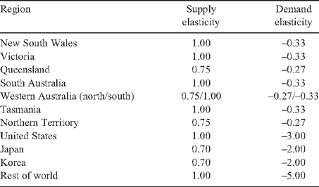
The base elasticity values are given in Table 2. These are taken mainly from Zhao et al. (2000). Note that the domestic demand elasticities given in Zhao et al. (2000) have been reduced by two-thirds to reflect the demand at the farm level modelled here rather than demand at the retail level modelled in that study. The demand elasticities are scaled down to reflect the ratio of the approximate farm price of $3/kg divided by the approximate retail price of $10/kg (ABARE 2007). The demand elasticities for the northern states have been set lower than those for the southern states because of fewer possible substitute products available to consumers. Also, the demand elasticities for the USA, Japan, Korea and the ROW are export demand elasticities for Australian product, and, therefore, have been set as being moderately to highly elastic because of the existence of many possible substitutes available to consumers and many possible sources of supply of beef.
|
Finally, the supply elasticities for the extensive northern states have been set lower than those for the southern states because of less flexibility in enterprise choices and expansion opportunities. The same reasoning holds for Japan and Korea compared with the USA and the ROW.
The relevant measures of K are defined in each of the scenarios that follow. The data in Tables 1 and 2 plus the relevant measures of K allow the DREAM software to calculate the gross annual benefits from a shift in supply brought about by the new technology outcomes generated by this project.
Information is also required on several other variables and parameters (Wood et al. 2001). Many of these were the same as those used in the Beef CRC renewal analysis:
-
the lag before the research results are available to cattle producers (1 year),
-
adoption lags (2 years until maximum adoption, to match the Beef CRC accelerated adoption objectives),
-
adoption levels (35%, to match the Beef CRC accelerated adoption objectives, but discounted back to 15% because many of the better producers will already have adopted this technology),
-
disadoption if relevant (not considered to be relevant in this study),
-
probability of success of the technology producing the expected outputs across all the target markets (80%),
-
the time period over which the outcomes are to be assessed (15 years),
-
the discount rate (7% real, to approximate the overdraft rate faced by commercial cattle producers),
-
the degree to which regions are linked together by prices (fairly closely – parameter value = 0.8 where 1.0 is a completely free market), and
-
whether the technology is to be available outside the region where the RD&E occurred [not considered to be available outside the region where the RD&E occurred, with the exception of the spillover of Vic. results to SA and Tasmania (Tas.)].
For a discussion of these issues see also Marshall and Brennan (2001).
Results
Growth rate comparisons
The first scenario examined is the comparison between slower and faster growth rates at each site, averaged across breed types and using the ‘traditional’ calving time in those states where this was varied.
For NSW, data from tables 4 and 5 in Davies et al. (2008) was used to calculate a minimum advantage of $37/steer for the fast treatment over the slow treatment across all breed types. This had to be done on a per head basis so that the feedlot and pasture phases could be aggregated. Based on the average slow growth slaughter weight of 355 kg, this advantage of $37/steer can be converted to 10.3 ¢/kg, or to 3.3% of the NSW equilibrium price of $3130/t defined in Table 1 above. The K-value is then 0.033 for NSW. This can be thought of as a 3.3% net reduction in the cost of producing a kg of beef in NSW from shifting from a slow to a fast growth path.1
Similarly for Vic., the information in table 6 in Davies et al. (2008) provided an advantage of $16/head for the fast treatment, autumn calving, for all breed types. For a mean carcass weight of 290 kg, this gave a K-value of 0.017, or a 1.7% reduction in the cost of producing beef in Vic. This value was also used for SA (where there was no growth path experimental data) and Tas. Finally, for southern WA, the information in table 7 in Davies et al. (2008) was used to calculate a K-value of 0.086, for the fast treatment across all breed types for autumn calving. This can be thought of as an 8.6% reduction in the cost of producing a kg of beef in southern WA.
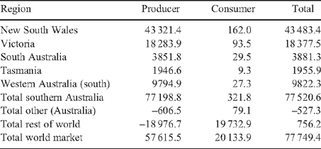
Inputting these K-values into the model together with the other data and parameters described above produced the results shown in Table 3. These values represent the accumulated value in 2000–01 dollars of the individual annual benefits to producers and consumers in each of the specified regions over the specified 15-year time horizon, discounted at 7%.
|
Therefore, using the model, data and assumptions described above, the aggregate benefits of an additional 15% of southern Australian beef producers moving from a slow (or conventional) growth path system to a faster growth path system is about $77.7 million over a 15-year time horizon. In terms of timing, the benefits are calculated to be $2.8 million after 1 year and $10.3 million after 5 years.
These benefits are caused by increases in the production of beef in the southern Australian states due to the now higher profitability of the cattle enterprises that take up the fast growth technology according to the assumptions about impact and adoption profile. This increased output causes beef prices to fall everywhere, since we specify a relatively free market structure. Almost all of the benefits accrue to southern Australian beef producers, as they have access to the new technology that more than compensates for the price fall. This works out at around $950 per 100 breeding cows (present value over the 15-year time horizon) for those producers who adopt the technology. Conversely, beef producers in the rest of Australia and the rest of the world lose, as they suffer the consequences of the fall in prices but do not have access to the technology. The other big winners are beef consumers in the ROW, who can now access greater quantities of beef at lower prices. However, the positive and negative market impacts outside of southern Australia essentially cancel each other out.
Time-of-calving comparisons
The second scenario examined is the comparison between calving times in those states where this was varied, averaged across breed types and using the ‘conventional’ slow growth rates at each site to avoid double counting.
For Vic., the information in table 6 in Davies et al. (2008) provided an advantage of $37/steer for the slow treatment, spring calving, for all breed types. For a mean carcass weight of 290 kg, this gave a K-value of 0.040, or a reduction in cost of production of 4.0%. This value was also used for SA and Tas. For southern WA, the information in table 5 in Davies et al. (2008) was used to calculate a K-value of 0.102 (a cost reduction of 10.2%), for the average across all breed types for winter calving.
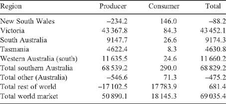
Inputting these K-values into the model together with the other data and parameters described above produced the following results as shown in Table 4.
|
Therefore, the aggregate benefits of an additional 15% of southern Australian beef producers (except those in NSW) moving from an autumn to a winter or spring calving time is about $69 million in present value terms over a 15-year time horizon. In terms of timing, the benefits are calculated to be $2.4 million after 1 year and $8.9 million after 5 years. Again, almost all of the benefits accrue to southern Australian beef producers (around $840 per 100 breeding cows). NSW beef producers appear to lose from this scenario, because there was no time-of-calving experiment in NSW and hence no measured cost saving. However, for NSW enterprises where time-of-calving principles and technology were considered applicable, similar benefits could be assumed to accrue.
Carcass/breed type comparisons
The third possible scenario to examine is the comparison between carcass/breed types, averaged across calving time in those states where this was varied and using the conventional slow growth rates at each site. However, a formal analysis would require data on the distribution of the various breed types in the different regions, and how these distributions might alter in the future. Further, examination of the results reported in Davies et al. (2008) and related papers suggests that in many cases there were no significant differences in gross margins across breeds, even though there were differences in many of the carcass characteristics. All we can do in the present paper is to highlight some of the breed type results that were different from the average, as a guide for producers who are considering changing breed types.
The NSW data identified weight gain as the biggest driver of profitability of production. The Charolais carcass type, even within the slower growth treatment, outgrew all other types in the sample of progeny groups in this experiment and was the most profitable on pasture. During feedlot finishing, the Charolais types achieved the best gross margin following slower pre-feedlot growth (due to high compensatory growth), but next to worst following the fast pre-feedlot phase. Although their growth rates in the feedlot stage were as high as for other breeds, there were additional feeding costs due to their higher average bodyweight. The higher feedlot entry weight also caused a higher initial ‘purchase’ price (hence interest bill) for the Charolais steers, but their outcome was also largely affected by their lower grid value (per kg) due to a high proportion having carcass weights over 380 kg. High growth breed types have much to offer in terms of overall profitability because of their extra weight at sale, but need to be managed carefully to ensure acceptable compliance for other traits. Further, where change of ownership occurs at the feedlot entry, there would seem to be an argument for feedlots to offer some incentives for producers to supply slower-growing animals within the high growth breed types.
Conversely, the Red Wagyu type was the slowest growing and performed worst in terms of gross margin. However, as with the Charolais, conclusions are restricted by the small sample of the sire type. The poor result may also be due to the specific post-feedlot specifications, and suggests again that different carcass types are relatively more or less suited to different market specifications.
The southern WA economic analyses confirmed these findings with the progeny of sires selected for high carcass yield having a slight advantage in overall value through their greater carcass weights. The Vic. site analyses also showed the importance of producing cattle with heavier slaughter weights, highlighted when comparing the Wagyu ($339/ha) to the other breeds ($373/ha) across all growth rates and times of calving. This was a $34/ha premium to the higher yielding sire classes. In SA, only the Angus breed was examined, but like the WA results, the progeny of sires selected for high carcass yield were clearly dominant (up to $17/ha).
Commercial v. research station
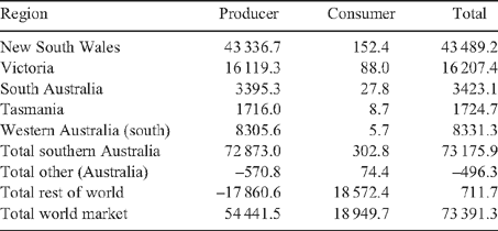
One issue related to defining the K-value (the impact of the technology on the per kg cost of production) is whether to apply the so-called Davidson and Martin (1965) discount. These authors argued that experimental results should be discounted by a factor of a third when they are applied in a commercial situation to reflect the higher levels of management and operating labour, the more timely application of inputs, and the overall higher quality of inputs, that are typically used in experimental protocols. In this project, the NSW site was a commercial beef property and a commercial feedlot was used to finish the animals, so no discount is required. In the other states, some parts of the experiment were conducted on partner agency research stations, so a 15% discount (an arbitrary 50% reduction) was applied. The results are reported in Table 5.
|
Compared with the outcomes reported in Table 3, it is evident that applying a partial Davidson and Martin discount for the lower outcomes expected in commercial relative to experimental situations does not materially impact on the overall benefits of the fast growth path technology.
Discussion and conclusions
Economic calculations regarding the profitability of different nutritional, genetic and time-of-calving combinations have been reported in Davies et al. (2008) and related papers for individual beef enterprises representative of four southern Australian production regions. In this paper, those results are aggregated up to the level of the Australian cattle and beef industry and then projected forward over several years into the future. To do this, an existing model of the world beef market is used.
The aggregate economic analyses suggest that both the fast-growth-rate technology and the time-of-calving technology have the potential to generate significant economic benefits for the southern Australian cattle and beef industries. The cumulative present values of each technology are around $70 million over a 15-year time horizon at a 7% real discount rate, with benefits in the first year of around $2–3 million and benefits after 5 years of around $9–10 million. Although not valued formally, it is evident that individual producers running specific breed types could also achieve greater returns by better targeting their cattle to appropriate markets that reflect the growth and carcass types they produce.
These are gross benefits in that they do not take account of the value of the additional investments required to shift into different growth paths, time of calving, or breed types. The values provide an upper bound to the aggregate level of investment in additional resources that could be made by southern Australian cattle producers. However, the general overall profitability of the fast growth alternative provides a level of confidence for producers to invest in pasture improvement, more targeted pasture management or supplementary feeding.
Several other summary points that have an economic context are worth making here. First, animals from slow growth paths still achieved satisfactory meat quality scores. This means that if cattle have been grown slowly before finishing, due to adverse seasonal conditions or other reasons, meat eating quality is unlikely to be adversely affected, unless age at slaughter is seriously delayed. This demonstrates a high degree of robustness in cattle growth paths capable of delivering acceptable eating quality.
Second, the regional nature of this RD&E program is expected to lead to more rapid adoption of the results. While this is difficult to quantify, there is already evidence that the time-of-calving results have encouraged a shift in breeding season in the south of WA. Similar outcomes should be evident at the other sites as the results are released.
Finally, the gross margin results reported in Davies et al. (2008) and related papers, and used as the basis for the industry benefit calculations reported here, provide a good guide for producers to select the most profitable combination of genotype, pasture management and market specification for them, and the best combination of inputs that will help them achieve a sustainable level of profit over the longer term.
Acknowledgements
The financial and in-kind support of the Cooperative Research Centre for Cattle and Beef Quality and its partner agencies is gratefully acknowledged. Thanks also to the many staff of these agencies that assisted in field operations, data collection and processing, biometrics and administrative support. The economics team pays a special tribute to the overall project management team of Bill McKiernan and Jim Walkley who provided support, data and other assistance whenever asked. Stuart Mounter and Kirrily Pollock provided valuable comments on an earlier draft of this paper.
Davidson BR, Martin BR
(1965) The relationship between yields on farms and in experiments. Australian Journal of Agricultural Economics 9(2), 129–140.
[Verified 9 March 2009]
Marshall GR, Brennan JP
(2001) Issues in benefit-cost analysis of agricultural research projects. The Australian Journal of Agricultural and Resource Economics 45(2), 195–213.
| Crossref | GoogleScholarGoogle Scholar |

McKiernan WA,
Wilkins JF,
Barwick SA,
Tudor GD,
McIntyre BL,
Graham JG,
Deland MPD, Davies L
(2005) CRC ‘Regional Combinations’ project – effects of genetics and growth paths on beef production and meat quality: experimental design, methods and measurements. Australian Journal of Experimental Agriculture 45, 959–969.
| Crossref | GoogleScholarGoogle Scholar |

1 The calculated K-values represent net reductions in variable costs as they are based on differences between steady state gross margins, and so reflect differences in both enterprise costs and returns between alternatives. However, they do not include any additional whole-farm costs, especially investment costs, required to implement the alternative production system (nor, any additional benefits derived from more efficient whole-farm input or output combinations).


