

Assessing the effect of marine isoprene and ship emissions on ozone, using modelling and measurements from the South Atlantic Ocean
J. Williams A K , T. Custer A , H. Riede A , R. Sander A , P. Jöckel A , P. Hoor A , A. Pozzer A B , S. Wong-Zehnpfennig A , Z. Hosaynali Beygi A , H. Fischer A , V. Gros C , A. Colomb D , B. Bonsang C , N. Yassaa A E , I. Peeken F G , E. L. Atlas H , C. M. Waluda I , J. A. van Aardenne J and J. Lelieveld AA Max Planck Institute for Chemistry, J. J. Becherweg 27, D-55128 Mainz, Germany.
B Energy, Environment and Water Research Center of the Cyprus Institute, 1645 Nicosia, Cyprus.
C Laboratoire des Sciences du Climat et de l’Environnement, Commissariat à l’Énergie Atomique (CEA), Centre National de la Recherche Scientifique (CNRS), Université de Versailles Saint-Quentin-en-Yvelines (UVSQ), F-91191 Gif sur Yvette, France.
D Laboratoire Interuniversitaire des Systèmes Atmosphériques, Unité Mixte de Recherche (UMR) 7583/CNRS, Université Paris 12, 61 av. Général de Gaulle, F-94010 Créteil, France.
E Present address: Faculty of Chemistry, University of Sciences and Technologie Houari Boumediene, University of Sciences and Technology Houari Boumediene (USTHB), B.P. 32 El-Alia, Bab-Ezzouar, 16111 Algiers, Algeria.
F Alfred Wegener Institute for Polar and Marine Research, Polar Biological Oceanography Am Handelshafen 12, D-27570 Bremerhaven, Germany.
G Present address: Center for Marine Environmental Sciences (MARUM), Leobener Strasse, D-28359 Bremen, Germany.
H Rosenstiel School of Marine and Atmospheric Science (RSMAS), University of Miami, 4600 Rickenbacker Causeway, Miami, FL 33149, USA.
I Biological Sciences Division, British Antarctic Survey, Natural Environment Research Council, High Cross, Madingley Road, Cambridge, CB3 0ET, UK.
J European Commission, Institute for Environment and Sustainability, I-21020 Ispra, Italy.
K Corresponding author. Email: williams@mpch-mainz.mpg.de
Environmental Chemistry 7(2) 171-182 https://doi.org/10.1071/EN09154
Submitted: 27 November 2009 Accepted: 17 February 2010 Published: 22 April 2010
Environmental context. Air over the remote Southern Atlantic Ocean is amongst the cleanest anywhere on the planet. Yet in summer a large-scale natural phytoplankton bloom emits numerous natural reactive compounds into the overlying air. The productive waters also support a large squid fishing fleet, which emits significant amounts of NO and NO2. The combination of these natural and man-made emissions can efficiently produce ozone, an important atmospheric oxidant.
Abstract. Ship-borne measurements have been made in air over the remote South Atlantic and Southern Oceans in January–March 2007. This cruise encountered a large-scale natural phytoplankton bloom emitting reactive hydrocarbons (e.g. isoprene); and a high seas squid fishing fleet emitting NOx (NO and NO2). Using an atmospheric chemistry box model constrained by in-situ measurements, it is shown that enhanced ozone production ensues from such juxtaposed marine biogenic and anthropogenic emissions. The relative impact of shipping and phytoplankton emissions on ozone was examined on a global scale using the EMAC model. Ozone in the marine boundary layer was found to be over ten times more sensitive to NOx emissions from ships, than to marine isoprene in the region south of 45°. Although marine isoprene emissions make little impact on the global ozone budget, co-located ship and phytoplankton emissions may explain the increasing ozone reported for the 40–60°S southern Atlantic region.
Introduction
Between January and March 2007, comprehensive ship-borne measurements of trace gases and aerosols were made while crossing the South Atlantic Ocean from South Africa to Chile and back as part of the OOMPH field experiment (Organics over the Ocean Modifying Particles in both Hemispheres, see www.atmosphere.mpg.de/enid/oomph, accessed 9 June 2009). The vessel traversed regions of relatively low marine biological productivity in the middle and South Atlantic, and a high productivity region of a natural phytoplankton bloom in the west (see Fig. 1a, b). A summary of mixing ratios of selected trace gases is given in Table 1, the data is divided into both bloom and remote conditions for leg 1, and for comparison the average of both legs shown in Fig. 1. Noteworthy are the extremely low mixing ratios observed for both NOx and the volatile organic species such as acetone and carbon monoxide. In particular, NOx was measured at ~10 ppt in the remote marine air. These NOx values are the first reported from a ship in the South Atlantic and are less than those measured at terrestrial surface sites, even at remote locations such as Antarctica.[1] Similarly, measurements of methanol and acetone, species that are ubiquitous in the atmosphere, were amongst the lowest recorded in the troposphere, comparable to measurements made in the remote Pacific.[2] Some organic trace gases, which are known to be emitted from the ocean (e.g. isoprene[3]), exhibited significantly elevated mixing ratios over the phytoplankton bloom regions. Nonetheless the trace gas composition of the marine boundary layer of the remote Southern Ocean can be considered as one of the most atmospherically pristine areas on Earth.

|

|
On 2 February 2007, while crossing the high chlorophyll region (around 46°S, 59.3°W) our research ship unexpectedly encountered between 150 and 200 vessels of the main high seas South Atlantic fishing fleet. The fleet was comprised mostly of Far Eastern squid fishing boats (jiggers) targeting the Argentine short finned squid Illex argentinus. These vessels operate mainly at night using large arrays of powerful lights, typically 150 bulbs of 2–3 kW, to lure squid to the ship,[4] see Fig. 2a. The fleet is a very strong light source by night and as a result is easily detectable in satellite imagery from the United States Air Force, Defence Meteorological Satellite Program Operational Linescan System (DMSP-OLS) (see Fig. 2b). The fishery operates over a wide area (42 to 53°S) and the movement of the fleet has been used to examine squid migration routes and to quantify fishing effort across the whole species range.[5,6] In order to operate in this manner the ships must generate considerable power (~1 MW per ship) and in doing so the ships release NOx (NO + NO2) into the otherwise pristine environment. In the first stage of this analysis we use an atmospheric chemistry box model (MECCA[7]), initialised where possible with field measurements and NOx emission estimates based on the observed fleet size, to assess the local impact of the ships’ NOx on ozone. In particular we examine the chemical consequences of this nocturnally emitted anthropogenic NOx in a region with diurnal natural emissions of isoprene. We then extend this local scale study of the fishing fleet to a regional scale by examining the contribution of ship transport to the NOx emissions inventory for the Southern Ocean region. Finally we employ the EMAC global model to gauge the sensitivity of global surface ozone to anthropogenic ship emissions (NOx) and natural phytoplankton emissions (using isoprene as a surrogate). The results are then discussed in the context of recently reported ozone trends and future emission scenarios.

|
Methods
GC-MS measurements
Isoprene was determined by GC-MS from air samples taken in canisters and cartridges. A separate inlet line for both canister and cartridge samples was installed at the top of the foremast (18 m above sea level). The canisters were filled to ~3 bar using a metal bellow pump, which was also used to flush the 1.27-cm outer diameter, 75 m-long, shrouded Teflon line thoroughly before sampling. The canisters were analysed by GC-FID and GC-MS, the analytical system is described elsewhere.[8,9]
For the cartridge samples air was drawn rapidly and continuously (at 7 L min–1) through a 1.27-cm outer diameter, 75 m-long, shrouded Teflon line. The residence time in the line was estimated as <1 min. Air samples were collected by drawing air at a flow rate of 50 mL min–1 through stainless steel, two-bed sampling cartridges (Carbograph I/Carbograph II; Markes International, Pontyclun, UK). Prior to air sampling, the sampling cartridges were cleaned with the Thermoconditioner TC-020 (Markes International, Pontyclun, UK). Cleaning was achieved by purging with helium 6.0 (99.9999%, Messer-Griesheim, Germany) for 120 min at 350°C and 30 min at 380°C. For storage the cartridges were sealed with brass caps with PTFE ferrules and put into an airtight metal container (Rotilabo, Carl Roth GmbH & Co, Karlsruhe, Germany). Shortly before the analysis, the brass caps were exchanged for DiffLok-caps (Markes International, Pontyclun, UK). More than 100 cartridges were sampled during the first leg of the OOMPH cruise, and on the second leg a further 100 samples were taken on-line with the GC-MS system described below.
The GC-MS analysis system used to analyse the cartridges consists of an air concentrating autosampler and a thermal desorber (Markes Int., Pontyclun, UK), coupled to a gas chromatograph (GC6890A, Agilent Technologies, CA, USA) linked to a Mass Selective Detector (MSD 5973 inert) from the same company. Laboratory multipoint calibrations showed good linearity within the concentration ranges measured. One-point calibrations of VOC standard (Apel-Riemer, CT, USA) were carried out at 2-h intervals. Blanks were taken regularly and showed no traces of isoprene. The total measurement uncertainty was between 10 and 15%, the detection limit ranged from 0.5 to 5 pptv.
Measurements of methanol, acetone and DMS (PTR-MS)
A proton transfer reaction mass spectrometer (PTR-MS) was employed to measure masses 33, 59 and 63 that have been attributed to methanol, acetone and DMS respectively. These identifications are in keeping with previous studies although minor contributions from other species, such as propanal to mass 59 cannot be ruled out.[10,11] The instrument was positioned in an air conditioned laboratory in the middle of the research vessel. Ambient air was drawn rapidly (~7 L min–1) and continuously from the top of the 18-m foremast through a 1.27-cm outer diameter and 75 m-long Teflon line, which was shrouded from sunlight. The inlet residence time was ~1 min. A fraction of this flow was sampled online by the PTR-MS. The entire inlet system of the PTR-MS including switching valves comprised of Teflon. Within the instrument, organic species with a proton affinity greater than water are chemically ionised by proton transfer with H3O+ ions and the products are detected using a quadrupole mass spectrometer.
Calibrations were performed during the campaign using a commercial gas standard (Apel-Reimer Environmental Inc.). The total uncertainties of the measurements are estimated to be 21.3, 15 and 14% for methanol, acetone and DMS respectively. This includes a 5% accuracy error inherent in the gas standard and a 2σ precision error for all the compounds. Detection limit was defined as the 2σ error in the instrument signal, while measuring methanol at an average mixing ratio of 1 ppb and each of the other compounds at an average mixing ratio of 0.5 ppb. The individually calculated precision errors and detection limits were as follows: methanol (16.3%; 0.24 ppb); acetone (10%; 0.07 ppb); isoprene (12%; 0.06 ppb); and DMS (9%; 0.05 ppb).
CO measurements
Atmospheric carbon monoxide was measured every five minutes with a gas-chromatograph equipped with a mercuric oxide reduction detector (Trace Analytical, USA), with the same principle as the instrument described in detail in Gros et al.[12] The limit of detection was 2 ppb with an overall uncertainty of 4%. Samples were calibrated against a certified NOAA standard (151.5 ppb).[13,14] Air was sampled from the east side of the vessel with a 20-m Teflon line (1/4′, 0.635 cm).
O3 measurements
Ozone was measured every minute with a UV-absorption instrument (model 49C, Thermo-Electron, USA). This type of instrument has shown good stability and reproducibility.[15] The estimated uncertainty is better than 5%. The instrument used aboard the Marion Dufresne was not calibrated before the campaign but a few months later by the EMPA laboratory (Duebendorf, Switzerland) and this calibration was applied to the Marion-Dufresne dataset. Air was sampled from the central inlet located at the top of the mast.
NOx measurements
The instrument used to measure NOx (NO + NO2) was a heavily modified ECOPHYSICS CLD 790, high resolution, high sensitivity 3-channel chemiluminescence detector capable of simultaneously detecting ozone (O3). The integration time of the original data is 2 s. However, for this case study the data has been averaged over 60 s. The detection limit (DL) of the measured species was determined based on the reproducibility of the Zero gas measurements carried out during field measurements on a daily basis throughout the campaign. The uncertainty is defined as the total sum of precision and accuracy for each separate channel. The precision was deduced from the sum of the DL and the reproducibility of the infield calibrations. The accuracy was calculated based on the total sum of the accuracy of the standard gas used and also the uncertainty due to the offset corrections. The uncertainty of NOx is calculated statistically from the uncertainty of the NO and NO2 measurements. The total uncertainty of the NOx data is 2.7 pptv + 6.2% of reading (2σ).
Satellite measurements
The image used in Fig. 2b was obtained from the Defence Meteorological Satellite Program Operational Linescan System (DMSP-OLS) at 0017 hours on 3 February 2007 (satellite F16). The image was georeferenced using algorithms developed by the National Geophysical Data Center (NGDC) Boulder, Colorado,[16] and incorporated into a Geographical Information System (GIS; ArcGIS, version 8.2); ESRI, Environmental Systems Research Institute, where it was converted to a mercator equal-area projection with a resolution of ~2.7 km. The DMSP-OLS visible band has 6-bit quantisation producing digital number (DN) values ranging from 0 (no radiance) to 63 (saturated radiance).[16] For each image, pixels with a DN value of ≥30 (i.e. the brightest 50% of lit pixels assuming an even split between lights from vessels and lights reflected from the ocean surface) were extracted and defined as being representative of fishing lights.
The satellite images of chlorophyll distribution used in Fig. 1 are from the MODIS (moderate resolution imaging spectroradiometer) instrument with 1 × 1-km resolution. (http://modis.gsfc.nasa.gov/, accessed 9 June 2009). Monthly averages are used by the global model.
Box model
The simulations presented in Fig. 3 were carried out using the atmospheric chemistry box model CAABA, which is based on the MECCA chemistry submodel[7] within the MESSy framework.[17] The chemical mechanism comprised tropospheric reactions including gaseous and aqueous phase chemical species, among them halogen compounds. Two aerosol modes were defined, a coarse mode representing sea salt aerosol, and a fine mode for sulfate aerosol. Initialising conditions were taken from the in-situ data where available, and values for the NOx emitted by ships from shipping statistics and the literature, see Results section. Prior to emissions, a spin-up time of two weeks allowed to equilibrate marine background conditions within the box model. Bloom emissions within the model included isoprene, acetaldehyde, acetone and DMS and lasted for a period of four days.
|
Global model
The EMAC model is a combination of the general circulation model ECHAM5,[18] (version 5.3.01) and the Modular Earth Submodel System[19] (MESSy; version 1.1). The description and evaluation of the model system are presented in, and references therein. More details about the model system can also be found at http://www.messy-interface.org (accessed 9 June 2009), where a comprehensive description of the model is provided. The simulation period presented here covers the 3 months of the OOMPH field intensive from January to March 2007. Dry and wet deposition processes have been extensively described elsewhere,[20,21] as has the emission procedure.[22] The chemistry is calculated with the MECCA submodel.[7] The applied spectral resolution of the ECHAM5 base model is T42, corresponding to a horizontal resolution of the quadratic Gaussian grid of ~2.8 × 2.8°. The applied vertical resolution that was used in this study consists of 31 levels (up to ~10 hPa) of which ~25 are located in the troposphere. The model setup includes feedbacks between chemistry and dynamics via the radiation calculations. We used the anthropogenic emissions from the EDGAR database[23] (version 3.2 ‘fast-track’) for the year 2000, but updated the traffic emissions for road, ship and aviation as described elsewhere.[24] For biomass burning emissions the Global Fire Emission Database (GFED) was used.
The emissions fluxes of marine isoprene were calculated with the AIRSEA submodel,[25,26] from the difference of isoprene concentrations between atmosphere and ocean. The concentrations of isoprene in the water were calculated from the World Ocean Atlas chlorophyll fields (which are seasonally averaged over December–January–February),[27] by applying the linear relationship between chlorophyll and isoprene described by Broadgate et al.[28] In comparison to the January 2007 MODIS satellite chlorophyll maps, and in-situ data from the ship, the WOA appears to underestimate the chlorophyll concentration in the ocean in the location of interest during summer (January) by a factor of ~30 (and consequently also isoprene). This is possibly due to the seasonally averaged fields in the WOA, excessive vertical mixing in the model or to a general underestimate of Southern Ocean chlorophyll by the WOA. In order to obtain a reasonable seasonal flux and to match the in-situ isoprene data in air, we multiply by 100 the fluxes calculated by the submodel AIRSEA.
Results
Local photochemical effects of ships and phytoplankton
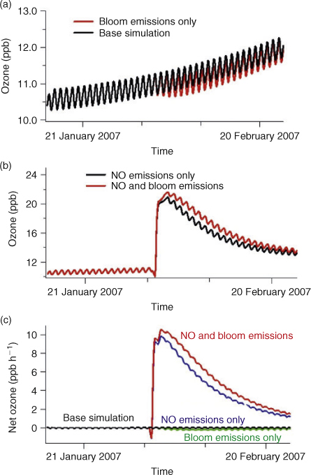
Based on comparable data from the international jigging fleet operating in Falkland island waters,[29] jigging vessels operating in the South Atlantic high seas region are likely to have a length of between 41 and 95 m (mean 58 m) with a gross registered tonnage of between 316 and 2495 t (mean 825 t) and possess a horsepower of 520 to 3330 hp (mean 1496; ~1 MW). Therefore the combined power consumption of the fleet in this region can reach 200 MW, comparable to a mid-size power station using low quality fuel and no emissions control technology. The estimated oil consumption in the region is 750 L fuel km–2 year–1,[30] which equates to regional levels of ~100 ppt of NOx in a 1 km-high marine boundary layer.[31] Ship NOx emissions in the box model (emitted as NO) were therefore implemented to occur between 2000 and 0440 hours local time, since the fishing vessels are active primarily by night, and an emission of 1 × 10¹¹ molecules cm–2 s–1 was set to occur at each model time step (20 min) so that a maximum mixing ratio of 1.1 ppbv is reached. This is in general agreement with previously reported ambient measurements of 0.5–2 ppbv NOx in ship plumes in the northern hemisphere.[32] Isoprene was emitted into the model by daylight in keeping with previous observations[3] to reach the levels measured during the cruise (see Table 1). Bloom emissions occurred for 4 consecutive days starting on 31 January at 0000 hours local time. Fig. 3a, b and c shows the results for ozone from the box model with initialising conditions representative of the South Atlantic region. Fig. 3a depicts the baseline simulation (without ship emissions), both with and without perturbation by marine organic species from the bloom. Fig. 3b shows the effect on ozone mixing ratios from NOx (input from ships), with and without bloom emissions. Fig. 3c shows the net ozone production rate (ppbv h–1) for all four cases depicted in Fig. 3a and b. Note that the small upward trend in the base simulation, Fig. 3a, is due to seasonal decreases in the ozone photolysis rate. Fig. 3a also shows that additional bloom emissions of isoprene, in the absence of significant NOx, serves to deplete ozone only slightly in the boundary layer compared to the base simulation. In contrast, the introduction of a single night of NOx emission from ships (midway in the simulation, Fig. 3b) leads to a sharp increase in ozone at daybreak. At this point the simulated ozone mixing ratios more than double from ~10 to 22 ppbv. This is due to organic compounds (e.g. methane or isoprene) reacting with OH to form peroxy radicals that react with the ship’s NO to form NO2. The NO2 photolyses by day to form oxygen atoms, which subsequently form ozone. Additional NOx increases the OH concentration and therefore decreases the NOx lifetime, which was estimated to be ~0.5 days before the NOx injection and 0.3 days between 1 and 3 days afterwards. The ozone levels reached when emissions of reactive isoprene from the bloom are included are greater than without (since more peroxy radicals are formed), although the difference between with and without bloom, is small in comparison to the overall ozone increase in both cases. This shows that the combination of anthropogenic NOx sources and biogenic marine VOC leads to efficient local ozone production, and that the juxtaposition of fishing boats emitting NOx over a natural marine bloom represents very favourable conditions for this process. From Fig. 3c it can be seen that the chemical influence of the NOx and VOC emissions persists for several days, giving elevated net ozone production rates, relative to the base case, until the NOx is removed. These conditions prevail for a limited time since the phytoplankton bloom is strongest in the Austral summer months and fishing continues from January to August being most active in February to May. NOx released by transport ships will, however, continue throughout the year and also produce ozone over the Southern Ocean. Many other squid fishing fleets operate globally, particularly in the Sea of Japan. However, emissions from such fleets occur into an already NOx rich atmosphere and so the effect on ozone is less pronounced.
Thus far we have examined the extreme case where the ships are only a source of NOx and the ocean is only a source of reactive hydrocarbon (isoprene). Ships do, however, also emit hydrocarbons into the atmosphere albeit in small amounts relative to NOx, SO2, CO and CO2.[31,33,34] Any significant emission of anthropogenic reactive hydrocarbons in the ships exhaust would moderate the relative effect of the biogenic VOC source discussed above, but still provide photochemical fuel for ozone production. Cruising vessels emit NOx and VOC in the ratio 24–36 : 1 by weight.[34] Thus according to the emissions databases for the fishing boat example given above, the 1 ppbv NOx plume should contain only ~28–42 pptv additional VOC and 200 pptv additional CO. On one occasion during this study the plume of a distant (~25 km) transporter ship was encountered on the open ocean and NO was observed to rise to between 200 and 500 pptv for 30 min. Unfortunately no canister and cartridge data were taken within this plume but no significant increases for benzene and toluene (by PTR-MS) were observed during this time. Although a comprehensive speciation of VOC from ship exhausts has not been found in the literature, the emitted VOC are likely to be predominantly aromatic compounds such as benzene, toluene, xylenes, etc.[31] These compounds and especially some of their oxidation products will tend to condense onto co-emitted aerosol, rather than react in the gas phase, particularly in the cold temperatures over the Southern Ocean. Therefore even the modest levels of isoprene detected over the large surface area sources of the Southern Ocean can play a role in photochemical ozone production where anthropogenic NOx is introduced.
Regional scale NOx and isoprene emissions
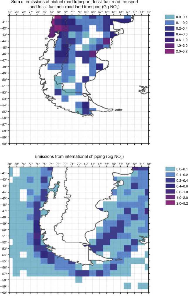
In this section we examine the spatial distribution, quantity and quality of ship NOx and marine isoprene emissions on the regional scale. Since fish abundances generally follow the regions of high phytoplankton and the fishing fleet follows the fish, NOx from fishing fleets will tend to be released in regions where marine phytoplankton also emit reactive hydrocarbons such as isoprene. As shown in the previous section this co-location of emission leads to efficient ozone production. In order to assess NOx emissions from transport ships we use the emissions database EDGAR (32FT2000),[23] and the regional terrestrial and marine NOx emissions are shown in Fig. 4. When the South American landmass south of 40°S is considered, the NO2 contributors from land transport (37 Gg NO2) and sea transport (31 Gg NO2) are approximately equal. However, as can be seen from Fig. 4, the emissions from ships become progressively more important further south, and are estimated to be the dominant NOx source south of 45°S. Furthermore, it should be noted that the NOx emissions from the transport ships operating along the South American coast do occur directly upwind of the large-scale phytoplankton bloom. Although NO2 has been measured from satellite measurements elsewhere in previous studies, a signal attributable to the fishing fleet discussed above or from the adjacent shipping lanes running parallel to the coast cannot be unequivocally identified in either SCIAMACHY or OMI output (not shown). The column densities expected for NO2 are insufficient to be discernable from the stratospheric NO2 column from space.
|
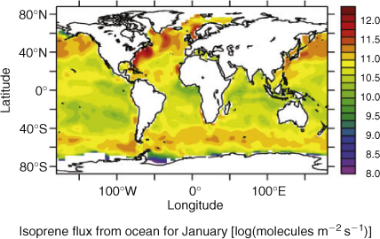
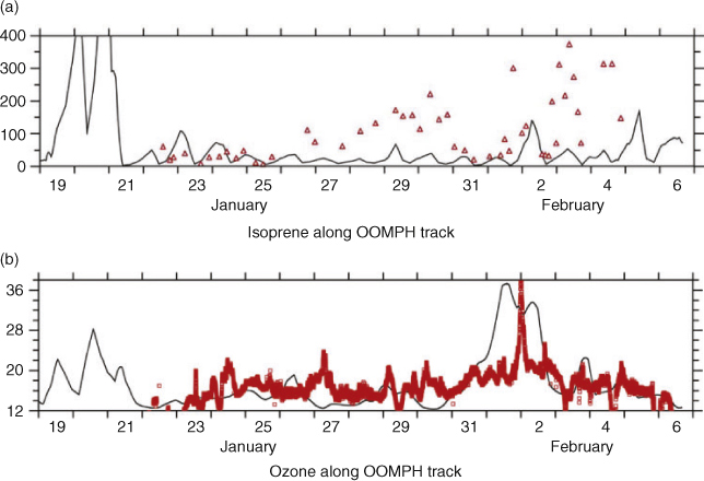
In the case of isoprene, fluxes have been estimated using the EMAC global atmospheric chemistry model based on satellite measured chlorophyll concentrations (World Ocean Atlas[27]) as described in the Global model section. Fig. 5 shows the global calculated fluxes for January, the southern hemisphere summer, and time of the OOMPH campaign. A broad band of emission is noticeable around the entire southern hemisphere between ~40 and 50°S corresponding to the region with high productivity and wind speeds. Particularly strong emissions can be seen in the region of the OOMPH cruise to the east of South America (co-located with the ship NOx emissions) and south-west of the Cape. The region of highest regional marine isoprene fluxes, south-west of South America is not currently co-located with significant ship traffic emissions. Surprisingly isoprene fluxes are calculated by the model to be higher in the North Atlantic than the South Atlantic even in January. This is as a direct consequence of the chlorophyll distribution in the World Ocean Atlas, and contrary to more recently reported seasonal chlorophyll distributions.[35,36] Initial comparisons between both the January 2007 MODIS satellite chlorophyll maps (see Fig. 1) and in-situ data from the ship, indicated that the model underestimated the chlorophyll concentration in the ocean, in the OOMPH cruise region during summer (January), by a factor of ~30. As described in the Global model section, this is possibly due to the 3-month (December–January–February) seasonally averaged chlorophyll fields in the WOA. As a result of these averaged chlorophyll fields and possibly other spatial and temporal averages inherent in the global model, marine isoprene surface mixing ratios from the EMAC model were found to be significantly less (factor 100) than the in-situ gas phase measurements. This suggests that the more recently reported chlorophyll distributions,[35,36] which exhibit significantly higher chlorophyll in the Southern Ocean, may represent reality better than the consolidated World Ocean Atlas on which the model is based. A further possibility is that the chlorophyll–isoprene relationship determined by Broadgate et al.[28] used as a basis in this model, is not suitable for these measurements. This seems less likely since both North Sea and Southern ocean data were used by Broadgate et al.[28] in their study. A final possible explanation of the discrepancy is the mixing used in the model. If the modelled MBL height is too high and mixing (between the MBL and free troposphere) is overestimated, then the predicted isoprene concentrations will be too low. In order to obtain a closer match to the in-situ isoprene data and to investigate the sensitivity of isoprene flux changes, we multiplied the isoprene fluxes calculated by the submodel AIRSEA by 100. A point to point comparison between the upscaled (×100) global model and the measurement data is shown for isoprene in Fig. 6a. Note that following the upscaling, the model mixing ratios were comparable, but still less than the measured values. The comparison between modelled and measured ozone during the OOMPH cruise was relatively insensitive to these isoprene flux scaling changes and modelled ozone mixing ratios were in reasonably good agreement with measured data even after isoprene emissions were upscaled by 100. A point to point comparison of modelled and measured ozone data is shown in Fig. 6b. From the comparisons of modelled isoprene with ship-borne measurements and modelled chlorophyll with satellite and in-situ measurements, both the spatial distribution and size of the model simulated fluxes must be considered rather uncertain. A further source of uncertainty is the parameterisation of the isoprene flux in terms of chlorophyll, which assumes stronger isoprene emitting phytoplankton species contain more chlorophyll. This is by no means certain although the chlorophyll parameterisation has been generally adopted in the absence of species specific emission rates. The measurements from the OOMPH cruise are in reasonable agreement with previous measurements from the Southern Indian Ocean (maximum values 280 pptv) and Southern Ocean (60 pptv) for which a correlation with chlorophyll was also noted.[37]
|
|
Global effect of marine isoprene and ship emissions on surface ozone
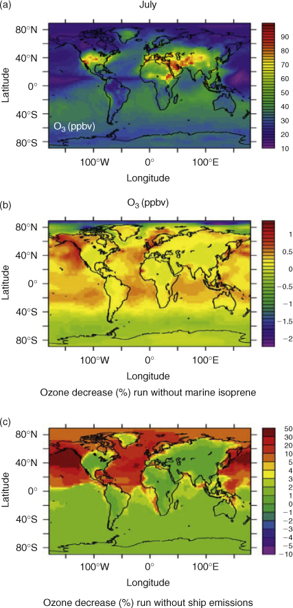
We now extend the study to the global scale and examine the relative impact of anthropogenic NOx emissions from ships and natural marine isoprene on ozone, for both January (time of the OOMPH campaign) and July (northern hemisphere summer) using the EMAC atmospheric chemistry model. Fig. 7 shows modelled data for January (the southern hemisphere summer and phytoplankton maximum) for (a) global map of surface ozone mixing ratios when ship emissions and marine organic emissions are included, (b) the percentage decrease in ozone (relative to a) when only marine isoprene emissions are removed and (c) the percent decrease in ozone (relative to a) simulated by the model when only ship emissions are removed. Fig. 8 shows the same plots but for July. Generally, when ship NOx was not emitted in the model, ozone decreases to a much greater extent than when marine emissions of isoprene are omitted. In July, marine boundary layer ozone decreases by a factor of 10–50% in the northern hemisphere and less than 5% in the southern hemisphere when ship NOx was excluded. In January, the absence of ship emissions leads to decrease of ozone of ~3–30% in the southern hemisphere with only a slight decrease observed in the northern hemisphere. The absence of isoprene emissions from the model, for either season and in either hemisphere affects ozone levels by only ±1–2%. This weak atmospheric impact of marine isoprene emission is consistent with the work of Arnold et al.,[38] who showed that global marine isoprene emissions also do not contribute significantly to organic carbon in marine aerosol. It is also consistent with the insensitivity of the ozone point-to-point comparison to the hundred fold scaling of the isoprene fluxes shown in the Regional scale NOx and isoprene emissions section. The initial total global emission of isoprene from the global model used here is 0.094 Tg year–1, which after upscaling becomes 9.4 Tg year–1. The un-scaled number (0.094 Tg year–1) is less than a recent bottom-up model budget (0.3 Tg)[38] suggests. However, the upscaled value is approximately five times larger than the top-down model budget estimate (1.9 Tg).[38]

|
|
Interestingly, for the region around Antarctica, removal of the marine emissions of isoprene leads to a slight increase in ozone levels (for both July and January) suggesting that in this pristine, low NOx region isoprene represents a direct sink for ozone, as observed in the simple box modelling study only, see Fig. 3a. Absolute changes in ozone in the global model must be interpreted with caution since the coarse resolution of the global model causes any given NOx emission to be instantly mixed across the model grid. This must be recognised as a limitation of the global model results since ozone production per NOx molecule is very sensitive to, and non-linearly dependent on, the ambient NOx level. Nonetheless the results show that the photochemistry of ozone in the remote marine boundary layer is much more sensitive to NOx emissions, the main source of which is ships; see the Regional scale NOx and isoprene emissions section, than from seasonal changes in marine isoprene emissions.
Recently, a 20-year ozone trend was reported for the marine boundary layer over the entire Atlantic region.[39] The region from 40 to 60°S was one of several identified where ozone had increased over the study period, by 0.17 ppbv year–1, i.e. ~30% since 1983, although no clear upwind terrestrial NOx sources were identified, that might explain this find. Ship traffic has been generally increasing in volume over this period,[31] indeed since the first world war, fuel consumption by ships has increased 4-fold.[40] Fish catch statistics for the south-west Atlantic have also increased significantly over the same 20-year period (~25%), in particular those of squid, cuttlefish and octopus.[41] From this study it seems likely that the observed trend in ozone is attributable to increases in NOx emissions through shipping and fishing co-located with marine emissions such as isoprene.
Conclusions
We conclude from these studies that NOx emissions from fishing generally and ship transport along routes adjacent to or over biologically productive waters are likely to produce more ozone than if the same emissions were made over oligotrophic ocean regions. The impact of these NOx emissions on ozone is therefore probably slightly underestimated in models without marine isoprene emissions, although in the global model the impact of marine isoprene emissions on surface ozone levels was found to be much less significant than current shipping emissions. From the model v. measurement comparison of isoprene shown here, we conclude that large uncertainties exist in modelled isoprene emissions in the marine boundary layer. Possible explanations for the low model estimated isoprene fluxes shown here, are that the seasonally averaged chlorophyll distribution in the World Ocean Atlas used in the model under-represents the real chlorophyll in the Southern Ocean or that the model overestimates vertical mixing between the MBL and free troposphere. Based on the local, regional and global study presented we suggest that the recently reported increase in marine boundary layer ozone over the South Atlantic over the past 20 years was caused, at least in part, by increases in ship NOx emissions, co-located with emissions of reactive VOC (e.g. isoprene) from phytoplankton.
Acknowledgements
The OOMPH project was funded under the EU sixth framework program (018419). The QUANTIFY project was funded by the EU within the sixth framework program under 003893. The authors are grateful for logistical support from the IPEV/Aerotrace program during the Southern Ocean cruise. In particular, we thank Jean Sciare for help with co-ordination and Roland Sarda-Esteve, Rolf Hofmann and Thomas Klüpfel for help with instrument operation.
[1]
A. M. Grannas ,
A. E. Jones ,
J. Dibb ,
M. Ammann ,
C. Anastasio ,
H. J. Beine ,
M. Bergin ,
J. Bottenheim ,
et al. An overview of snow photochemistry: evidence, mechanisms and impacts.
Atmos. Chem. Phys. 2007
, 7, 4329.
|
CAS |
[Verified 9 June 2009]
[24]
P. Hoor ,
J. Borken-Kleefeld ,
D. Caro ,
O. Dessens ,
O. Endresen ,
M. Gauss ,
V. Grewe ,
D. Hauglustaine ,
et al. The impact of traffic emissions on atmospheric ozone and OH: results from QUANTIFY.
Atmos. Chem. Phys. 2009
, 9, 3113.
|
CAS |

[25]
A. Pozzer ,
P. Jöckel ,
R. Sander ,
J. Williams ,
L. Ganzeveld ,
J. Lelieveld ,
Technical note: The MESSy-submodel AIRSEA calculating the air-sea exchange of chemical species.
Atmos. Chem. Phys. 2006
, 6, 5435.
|
CAS |
[26]
[27]
[28]
W. Broadgate ,
P. Liss ,
S. A. Penkett ,
Seasonal emission of isoprene and other reactive hydrocarbon gases from the ocean.
Geophys. Res. Lett. 1997
, 24, 2675.
| Crossref | GoogleScholarGoogle Scholar |
CAS |
[29]
[30]
P. H. Tyedmers ,
R. Watson ,
D. Pauly ,
Fueling global fishing fleets.
Ambio 2005
, 34, 635.
| PubMed |
[31]
V. Eyring ,
H. W. Köhler ,
J. van Aardenne ,
A. Lauer ,
Emissions from international shipping. 1. The last 50 years.
J. Geophys. Res. – Atmos. 2005
, 110, D17305.
| Crossref | GoogleScholarGoogle Scholar |
[32]
G. Chen ,
L. G. Huey ,
M. Trainer ,
D. Nicks ,
J. Corbett ,
T. Ryerson ,
D. Parrish ,
J. A. Neuman ,
et al. An investigation of the chemistry of ship emission plumes during ITCT 2002.
J. Geophys. Res. – Atmos. 2005
, 110, D10S90.
| Crossref | GoogleScholarGoogle Scholar |
[33]
Ø. Endresen ,
E. Sørgård ,
J. K. Sundet ,
S. B. Dalsøren ,
I. S. A. Isaksen ,
T. F. Berglen ,
G. Gravir ,
Emission from international sea transportation and environmental impact.
J. Geophys. Res. – Atmos. 2003
, 108, 4560.
| Crossref | GoogleScholarGoogle Scholar |
[34]
C. Deniz ,
Y. Durmusoglu ,
Estimating shipping emissions in the region of the Sea of Marmara, Turkey.
Sci. Total Environ. 2008
, 390, 255.
| Crossref | GoogleScholarGoogle Scholar |
CAS |
PubMed |
[35]
S. Dasgupta ,
R. P. Singh ,
M. Kafatos ,
Comparison of global chlorophyll concentrations using MODIS data.
Adv. Space Res. 2009
, 43, 1090.
| Crossref | GoogleScholarGoogle Scholar |
CAS |
[36]
B. Gantt ,
N. Meskhidze ,
D. Kamykowski ,
A new physically-based quantification of marine isoprene and primary organic aerosol emissions.
Atmos. Chem. Phys. 2009
, 9, 4915.
|
CAS |
[37]
Y. Yokouchi ,
H. J. Li ,
T. Machida ,
S. Aoki ,
H. Akimoto ,
Isoprene in the marine boundary layer (Southeast Asian Sea, eastern Indian Ocean, and Southern Ocean): comparison with dimethyl sulfide and bromoform.
J. Geophys. Res. – Atmos. 1999
, 104, 8067.
| Crossref | GoogleScholarGoogle Scholar |
CAS |
[38]
S. R. Arnold ,
D. V. Spracklen ,
J. Williams ,
N. Yassaa ,
J. Sciare ,
B. Bonsang ,
V. Gros ,
I. Peeken ,
et al. Evaluation of the global oceanic isoprene source and its impacts on marine organic carbon aerosol.
Atmos. Chem. Phys. 2009
, 9, 1253.
|
CAS |
[39]
J. Lelieveld ,
J. van Aardenne ,
H. Fischer ,
M. de Reus ,
J. Williams ,
P. Winkler ,
Increasing ozone over the Atlantic Ocean.
Science 2004
, 304, 1483.
| Crossref | GoogleScholarGoogle Scholar |
CAS |
PubMed |
[40]
Ø. Endresen ,
E. Sørgård ,
H. L. Behrens ,
P. O. Brett ,
I. S. A. Isaksen ,
A historical reconstruction of ships’ fuel consumption and emissions.
J. Geophys. Res. – Atmos. 2007
, 112, D12301.
| Crossref | GoogleScholarGoogle Scholar |
[41]
[42]
S. R. Zorn ,
F. Drewnick ,
M. Schott ,
T. Hoffmann ,
S. Borrmann ,
Characterization of the South Atlantic marine boundary layer aerosol using an aerodyne aerosol mass spectrometer.
Atmos. Chem. Phys. Discuss. 2008
, 8, 4831.