

Establishment of reference or baseline conditions of chemical indicators in New Zealand streams and rivers relative to present conditions
R. W. McDowell A E , T. H. Snelder B , N. Cox A , D. J. Booker C and R. J. Wilcock DA AgResearch, Invermay Agricultural Centre, Private Bag 50034, Mosgiel 9011, New Zealand.
B Aqualinc Research, PO Box 20-462, Bishopdale, Christchurch 8543, New Zealand.
C National Institute of Water and Atmospheric Research Limited, PO Box 8602, Riccarton, Christchurch, New Zealand.
D National Institute for Water and Atmospheric Research, PO Box 11-115, Hamilton, New Zealand.
E Corresponding author. Email: richard.mcdowell@agresearch.co.nz
Marine and Freshwater Research 64(5) 387-400 https://doi.org/10.1071/MF12153
Submitted: 14 June 2012 Accepted: 27 December 2012 Published: 3 May 2013
Journal Compilation © CSIRO Publishing 2013 Open Access CC BY-NC-ND
Abstract
The management of streams and rivers can be aided by knowledge of reference conditions. Data from >1000 sites across New Zealand was used to develop a technique to estimate median ammoniacal-N, clarity, Escherichia coli, filterable reactive phosphorus, nitrate-N, suspended solids, and total nitrogen and phosphorus values under reference conditions for streams and rivers as classified by the River Environment Classification (REC). The REC enabled us to account for natural variation in climate, topography and geology when estimating reference conditions. Values for minimally disturbed sites (i.e. <5% in intensive agriculture) were generally within the confidence limits for estimated reference values. Metrics that described: (1) the percentage of anthropogenic contribution to analyte values; and (2) the degree of enrichment beyond the reference conditions, showed that lowland sites classified as warm-wet, warm-dry or cool-dry exhibited the greatest anthropogenic input and enrichment. The consideration of natural variation by REC class informs the setting of water quality objectives through avoiding water quality limits or targets that are either too restrictive, and impossible to meet (e.g. below reference conditions), or too high, such that they have little ecological benefit. We recommend reference conditions be considered by regulatory authorities when assessing water quality impacts, objectives and limits.
Additional keywords: anthropogenic, clarity, contamination, enrichment, faecal bacteria, nitrogen, phosphorus, reference conditions, river assessment, sediment, water quality target.
Introduction
A key issue in the management of aquatic systems is the establishment of reference conditions. Reference conditions can be defined as the chemical, physical or biological conditions that can be expected in streams and rivers with minimal or no anthropogenic influence (Soranno et al. 2011). There is a need to establish the reference condition because it provides a baseline from which to compare changes in water quality parameters (e.g. analytes). However, the establishment of reference conditions through the selection of reference sites is problematic as few catchments are minimally affected by human activities. Reference conditions also define aspects of the physical habitat for maintaining a biological community and integrity (Dodds and Welch 2000). However, due to their ease of measurement, a much wider body of work has defined reference conditions for chemical and physical (viz. abiotic) factors used as surrogates for, or in addition to, biological indicators (De Pauw and Roels 1988). Hence, while we refer to chemical analytes under reference conditions in the present study, we are cognisant of their linkage to the broader definition.
The requirement to set or acknowledge reference conditions is enshrined in policy or law for many countries (e.g. US Clean Water Act), bilateral agreements (e.g. Australian and New Zealand guidelines for fresh and marine water quality; ANZECC 2000), or political unions (e.g. the European Union’s Water Framework Directive). Reference conditions are then used to detect and direct the control of anthropogenic inputs in the form of actions, such as maximum permissible annual loads or median concentrations (Reynoldson et al. 1997). However, it is important to recognise that natural background impact will vary between reference sites due to many factors such as topography, soil type rainfall and geology (Sánchez-Montoya et al. 2012), or over time. For example, Scarsbrook et al. (2003) found that over a 13-year period, temporal variability in 12 water quality variables showed an association with the Southern Oscillation Index that differed depending on which of six climatic regions the site was located in.
It is important that reference conditions are estimated as accurately as possible. This avoids establishing standards that are not achievable because natural background levels are already high, or alternatively, that are insufficiently protective of the environment. Accurate estimation of reference conditions provides information on the manageable portion of anthropogenic losses by identifying catchments where the manageable portion is: (1) so small that the practices necessary to reach acceptable levels would preclude human activities; or (2) very large and achievable at little or no cost, highlighting the potential for restoration of environmental conditions or intensification of human activities.
There is a range of methods used to estimate reference conditions. Statistically, the simplest is the ‘minimally disturbed condition’ (Lewis et al. 1999). The minimally disturbed condition approach utilises data from a stream or river that is not subject to anthropogenic disturbance now or in the past (Stoddard et al. 2006). However, such reference sites are uncommon, particularly in most agriculturally productive landscapes (Larned et al. 2003). Their rarity often means that a reference site may only be representative of a few catchments in the area due to differing climate or soil factors. Another approach for estimating reference conditions, known as the ‘historical condition’, uses data from before a stream or river became degraded (Stoddard et al. 2006). However, this approach may be unreliable because there is often little historical data and because of time lags between losses from agricultural land and the contamination of rivers and streams (Cooper and Thomsen 1988; Vant and Huser 2000). Another approach to the estimation of reference conditions is to combine sample data from reference sites in groups defined by a classification system and use a percentile of the distribution of values as the reference condition estimate (e.g. the 80% percentile of a large-undisturbed river as per ANZECC 2000). The quality of the estimate in this approach is limited by the ability of the classification system to group reference sites that are representative of the impact site. Alternatively, the ‘least disturbed condition’ also groups sample data for sites according to a classification and then nominates sites that have the least anthropogenic input (Stoddard et al. 2006). A reference condition is then estimated as a percentile at the lower end of the distribution of values for the least impacted sites (e.g. 5th percentile). Ideally, these three approaches are combined with an assessment of ecological conditions (e.g. including biological indicators). However, congruent ecological and water quality data are often lacking. Therefore all approaches, especially the least disturbed condition, run the risk of estimating a reference condition that is too high.
All of the above approaches to estimation of reference conditions are limited by both a lack of sampling sites that represent reference conditions, and a paucity of data. Dodds and Oakes (2004) among others (for review of these see Hawkins et al. 2010) developed a statistical approach that estimates the influence of anthropogenic land uses on nutrient concentrations in lotic systems. The approach utilised an analysis of covariance and linear regression to establish a relationship between nutrient concentrations and the percentage of anthropogenic land use for a range of sites that exhibit no significant regional effect (i.e. enabling sites to be aggregated between regions, thereby maximising the value of the data). The intercept of these regression relationships is the estimated nutrient concentration without anthropogenic influence, or a reference nutrient concentration.
In New Zealand, water quality guidelines (ANZECC 2000) refer to trigger values, which are the 80th percentile of the values measured at reference sites for stressors that are harmful at high concentrations (e.g. nitrate), or 20th percentile for stressors that cause problems at low concentrations (e.g. dissolved oxygen concentration). The guidelines present ‘default’ trigger values (i.e. to be used in the absence of a location specific estimate of the trigger value). These default trigger values were derived from distributions of values measured at baseline and pseudo-baseline sites within the National River Water Quality Network (Smith and McBride 1990). Distributions were obtained from data measured at sites in large streams and rivers in 18 upland (>150-m elevation and with glacial and lake-fed sites removed) and three lowland (<150-m elevation and with one site with alpine headwaters removed) locations. Hence, it could be argued that the default trigger values have very little discrimination of environmental variation (i.e. simply upland and lowland categories). This would be especially true for lowland sites, which are likely to be more impacted and variable due to anthropogenic inputs. The objective of the present study was to estimate reference conditions for analytes representing water quality (largely nutrients, sediment or faecal indicator bacteria) in streams and rivers in New Zealand at the finest possible resolution of environmental variation. We hypothesised that accounting for natural variation in reference conditions will better define the anthropogenic loss. This will aid in estimating the proportion of the total load that could be mitigated (manageable loss). To do the analysis, we collected data at more than 1000 sites that were routinely monitored by local and regional government for the last decade (up to 2009) and compared the approach developed by Dodds and Oakes (2004) to a new approach to estimating median analyte concentrations under reference conditions as classified by an environmental classification, the River Environment Classification (REC).
Materials and methods
Data sources, classification and initial filters
A database containing water quality data representing several analytes was collated from McDowell et al. (2009) and the National River Water Quality Network (NRWQN; for description see Smith and McBride 1990). This database included ~1000 sites sampled by Regional Authorities and 77 sampled by the National Institute of Water and Atmospheric Research. Data from 1989 to 2009 was used. All analytes were regularly measured during that time except Escherichia coli (E. coli), which has only been analysed periodically by Regional Authorities and within the NRWQN since 2005 (Ballantine and Davies-Colley 2009).
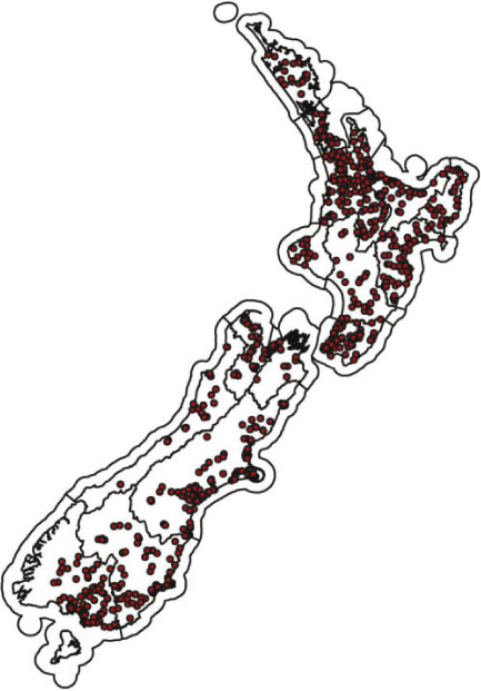
Spatial and temporal coverage varied despite the large size of the dataset. For instance, sampling frequencies vary from fortnightly to bimonthly. The sites in our dataset also tended to represent locations where Regional Authorities were either investigating a possible change in water quality or were likely to quickly reflect any change in, for example, land use. Sampling constraints, such as lack of funds or ease of accessibility, mean that geographical and environmental coverage of the sites is uneven and variable (Fig. 1).
|
We used the New Zealand REC (Snelder and Biggs 2002) to classify the sites according to the environmental conditions that are strong determinants of baseline water quality. Building on experience gained in earlier attempts (e.g. Biggs et al. 1990), the REC categorises rivers and streams according to overarching factors that are likely to influence biological and physical processes. The spatial framework for the REC is a digital representation of the New Zealand river network, comprising 560 000 segments (between confluences) with a mean length of ~700 m that is contained within a Geographic Information System. The first three levels of the REC focus on climate, topography, and geology of the catchment upstream of all network segments. Subsequent work has validated the REC in relation to flow (Snelder et al. 2005), nutrients (Snelder et al. 2004a), water quality (Larned et al. 2003), and invertebrate community composition (Snelder et al. 2004b). Being hierarchical, the REC enables the classification of all streams and rivers in New Zealand at varying levels of classification detail, from general to specific.
Site geographic coordinates and names were used to identify the REC class at the first three levels (climate, topography, and geology) for the segments on which each site was located (Table 1). The proportion of the area contributing catchment in categories defined by the New Zealand Land Cover Database (MfE 2004) was also obtained for each segment from the REC database. Previous work by Unwin et al. (2010) not only identified the percentage of intensive agriculture (originally listed by Unwin et al. (2010) as heavy pasture, due to the dominance of high-producing, exotic grassland, but also included small areas of cropland, vineyards, orchards) or urban land cover as the land uses with the most important predictors of water quality. Only a few sites had a high proportion of urban land use. After inspecting scatter plots of values, sites with >50% urban land use deviated significantly from the general relationship between % intensive agriculture and analyte values and were excluded from further analysis.

|
Analytes included in the analysis were clarity (reported in m), E. coli (measured as a most probable number (MPN) of E. coli cells 100 mL–1), suspended solids, filterable (also called dissolved) reactive phosphorus (FRP), total phosphorus (TP), nitrate-nitrogen (NO3-N), ammoniacal-nitrogen (NH4-N), and total nitrogen (TN) (all reported in g m–3). The following conventions were used to filter data:
-
Sites were only included in the database if there were 15 or more observations of an analyte during the period of record to ensure accurate estimates of median values for each variable at each site.
-
Analytes values below the indicated detection limit were set at half the detection limit. At some sites, the median value was below the stated detection limit. This was particularly the case for NH4-N, for which 17.4% of sites had median values below the detection limit. The proportion was less than 1% for all other analytes except FRP (4.3%) and suspended solids (3.4%). For analytes marked as in-excess of a specified level, such as E. coli (20 000 MPN 100 mL–1), the numerical value was used, but this was rarely (<2% of observations) the case. Note also that in some cases detection limits were not the same for all authorities or over time.
-
Ten sites were removed from the analysis which had greater than 50% urban land-cover in their upstream catchment. This was because these sites had the potential to bias the relationship between water quality parameters and intensive agriculture, which was the main focus of the present study.
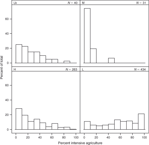
The data represented many sites, but not all analytes were observed, or were above the detection limit, on all occasions at all sites. Furthermore, sites were not equally distributed among REC classes (Fig. 2). To decrease this imbalance, we amalgamated the sites in the glacial mountain topography category of the REC into the mountain category. There were relatively few sites in these categories (~10 and 20, respectively) and because these two categories represent similar environmental mountainous catchment conditions, water quality can be expected to be similar (Larned et al. 2003).
|
Statistical analysis
In the analyses that follow, sites were treated as independent data and values at each site were represented by medians for each analyte. We note that 20 out of the 768 filtered sites used in the analysis were located on the same river segment, but as this represents only 2% of sites it is not expected to bias the analysis. We log (base 10) transformed the median value for each analyte before analysis to approximate normality and confirmed this with a Shapiro–Wilk test.
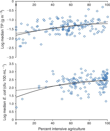
The analysis of covariance (ANCOVA), used in other studies (e.g. Dodds and Oakes 2004), determines if there is a linear relationship between the response (i.e. our logged median values of the analytes) and the explanatory variable (i.e. percent intensive agriculture) and whether this relationship differs between groupings of the data based on a factor (i.e. the REC classes). The statistical significance of the factor within an ANCOVA model justifies the amalgamation or separation of data based on REC class. However, if relationships are non-linear, especially where the percentage of intensive agriculture is low, ANCOVA models may poorly estimate the intercept (the value of interest representing the reference condition). Thus, we performed a preliminary step in which we inspected scatter plots of the logged median values of the analytes against the percent intensive agriculture for evidence of non-linearity in the relationships.
We then used a mixed-effects model with random slopes and intercepts, and with a smoothing spline (Verbyla et al. 1999), to model the relationship between the logged median values of each analyte and the percentage of intensive agriculture. The benefit of including a spline in the mixed-effects model is that it represents some non-linearity in the relationship. The benefit of fitting the random terms is that some information is gleaned from the data on all classes to aid the estimation on each class. Where a class has little data, the data from the other classes becomes more important and pulls the individual class estimate towards the mean of the other classes. However, a class with sufficient data for estimating the intercept will not be noticeably affected by the data from the other classes. Hence a mixed-effects model means that data from classes with few data are not discarded. Tests for the significance of the variation between REC (2nd level) classes for slope and intercept estimates as fitted as random effects used the likelihood ratio test (Verbyla et al. 1999).
Geology influences the concentration of certain analytes in water (e.g. P; Dillon and Kirchner 1975). To determine variation in estimating reference conditions due to geology, we took those REC classes at the second level (climate by topography) with the largest number of sites (i.e. cool-dry hill, cool-dry lowland, cool-wet hill, cool-wet lowland, cool-extremely wet hill, cool-extremely wet lowland, warm-dry lowland and warm-wet lowland; Table 1) and further analysed (as above) sites grouped at the third (climate by topography by geology) level of the REC provided there were five or more sites within each geology class.
The uncertainty of estimated reference conditions (i.e. the intercepts) is a reflection of the strength of the relationship between the analyte and percentage of intensive agriculture and the number of contributing sites. This was determined by the width of the 90% confidence intervals of the intercept terms in the models. We also assessed the reliability of the estimates of reference condition by comparing, where possible, the regression intercepts of the ANCOVA and mixed-effects models with concentrations at sites that were nominated as being in a minimally disturbed condition. For this comparison, we used the median value of sites with <5% intensive agriculture as minimally disturbed condition reference sites. Herlihy and Sifneos (2008) highlighted some of the disadvantages with this definition of a minimally disturbed condition reference site. For example, analyte values may be compromised if the 5% of intensive agriculture included in the definition surrounds the sampling site. Suplee et al. (2007) provided additional criteria to defend their selection of minimally disturbed condition reference sites for nutrients. This included the enrichment of other analytes such as heavy metals (or Al), in the presence of abandoned mines, and the use of best professional judgement to account for the presence of point sources or grazing impacts. Our criteria for sites categorised as minimally disturbed condition does not guarantee that sampling points were not near to intensive agriculture. However, we added to the stringency our minimally disturbed condition categorisation with an additional test. For all sites having catchment land cover of <5% intensive agriculture, we considered whether analytes exceeded current guidelines for good water quality in upland and lowland rivers in Australia and New Zealand (ANZECC 2000). Sites were then discarded as a minimally disturbed site if they exceeded the guidelines for any analyte. The exception to this was clarity and suspended solids for the mountain and lake classes, which were both allowed to exceed their ANZECC (2000) guidelines due to natural processes affect these analytes (e.g. glacial rock flour).
The models were fitted in Genstat 12 (GenStat Committee 2010) using residual maximum likelihood. The estimates generated by the ANCOVA procedure of Dodds and Oakes (2004) were also compared with the minimally disturbed condition-reference.
Analysis of anthropogenic influence
Estimates of the reference condition can be used to determine the degree of anthropogenic influence on water quality (e.g. McDowell et al. 2011). We used the reference condition estimates to define two metrics that quantify the degree of anthropogenic influence on streams and rivers. The first metric was the anthropogenic contribution to the analyte values. This metric was calculated by subtracting the estimated reference condition value from the median value at each site and expressing the remainder as a percentage of the site median value. We grouped these site indices by REC classes (2nd level) and reported the median values by analyte. The REC class values by analyte were compared by ranking and a one-way analysis of variance with pair-wise tests of the two most enriched classes with the remaining classes. The second metric was the degree of enrichment and was calculated by expressing the site median analyte value as a proportion of the estimated reference value of the analyte for the site. We reported the median values of these site indices by analyte in REC classes (2nd level) and the median values of each analyte across all sites.
Results
Estimation of analyte values under reference conditions
There were differences between linear and non-linear fits to the relationship between analyte and percentage intensive agriculture (Fig. 3). There tended to be a large number of sites with a high percentage of intensive agriculture and few with low percentages of intensive agriculture (Fig. 3). This increased the possibility that linear regressions would be affected by a ‘pan handle’ effect, i.e. insufficient leverage of sites with a low percentage of intensive agriculture so that the value of the intercept is overestimated. The non-linear spline fits reduced the possibility of insufficient leverage towards the intercept and underestimation of reference conditions. Using the mixed effects model, there were significant differences in the slope and intercept for all analytes for classes at the 2nd level of the REC (excluding slope for NH4-N, P = 0.500). For the 111 cases (out of a possible 144 REC by analyte combinations) where we had minimally disturbed condition reference values (i.e. median values of analytes for sites with <5% intensive agricultural land cover), 90 (81%) lay within the confidence limits for the intercept (i.e. the estimated reference condition) calculated using the mixed-effects models and a spline, whereas only 75 (68%) cases fell within the confidence intervals when the ANCOVA approach (implying a linear regression) was used.
|
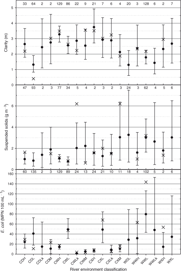
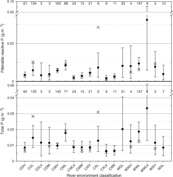
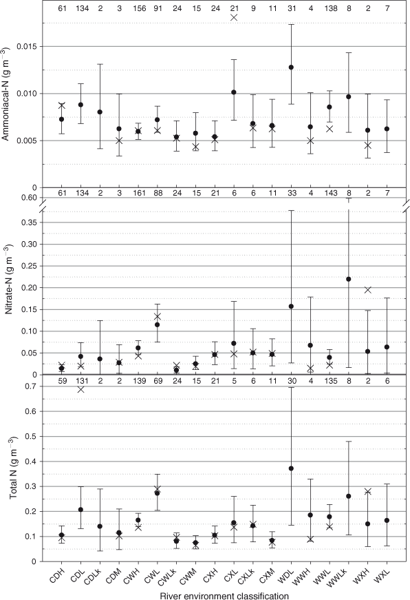
In general, confidence intervals were greater for warm REC climate level classes than cool classes (Figs 4–6). Often this was a reflection of a paucity of data (viz. <10 sites), but for some classes some analytes, such as E. coli and suspended solids, had wide confidence intervals despite being represented by more than 100 sites (Fig. 4). Across all classes, confidence intervals appeared widest for suspended solids and ammoniacal-N (Figs 4 and 6). One reason for wide confidence intervals may be the number of sites with median concentrations that are at or below the detection limit, especially if these occur across a wide span of percentage of intensive agriculture.
|
|
|
Sites belonging to Lake, Hill and Low-elevation REC topography categories covered a broad range of percentage of intensive agriculture. However, all sites in the mountain or glacial-mountain category had very low percentages of intensive agriculture. However, for cool-dry lowland where there was both ample data (>130 sites) and narrow confidence intervals compared with other classes, the minimally disturbed condition reference values for E. coli, FRP, TP and clarity sat outside the confidence intervals of the mixed-effects models (Figs 4 and 5). Visual inspection of the data indicated an even spread across percentages of intensive agriculture; including those with <2% per cent intensive agriculture, decreasing, but not eliminating, the potential for the estimate to be affected by a ‘pan handle’ effect. Thus, we suggest that there are either additional factors at play within this class (perhaps geology), or the reference sites were unrepresentative of this class.
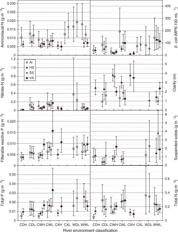
Estimates of reference conditions were made for up to four of the 3rd (geology) level REC classes within each of the amenable 2nd level REC classes (i.e. that conformed to data requirements; see materials and methods) (Fig. 7). Differences among geological classes appeared most likely for cool-wet lowland and warm-wet lowland sites based on minimal or no overlap of some confidence intervals. This suggested that minimally disturbed condition sites within cool-dry lowlands were potentially unrepresentative of the class at the second level of the REC. Most of the other classes exhibited either too few sites to yield more than one or two geological classes, or had widely overlapping confidence intervals. The cool-wet lowland sites exhibited greater FRP and TP for sites categorised as volcanic acid than sites of other geology categories, but this was not true of other analytes. Although warm-wet lowland sites categorised as hard sedimentary geology had greater TP than other geological categories, a clearer difference was exhibited by sites categorised as soft sedimentary geology, which had higher suspended solids, and lower clarity, than other sites in other geological categories.
|
Analysis of anthropogenic influence
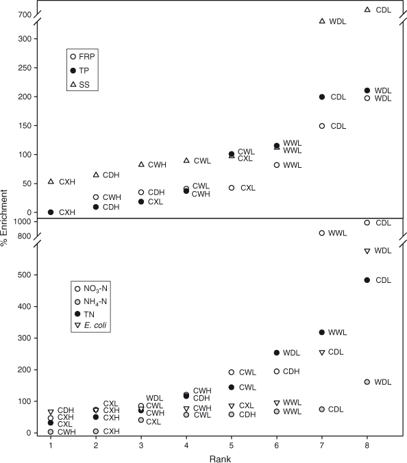
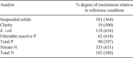
Compared with other REC classes, there were large differences in anthropogenic contribution to FRP, E. coli, suspended solids, TN and TP in the cool-dry lowland and warm-dry lowland classes (Table 2). The warm-wet lowland class also had larger anthropogenic contributions to TN and NO3-N than other classes (Table 2). Due to the large median concentration exhibited by most sites relative to their estimated reference condition, there were similar differences between classes for the degree of enrichment (Fig. 8). Across all sites, the median values for the degree of enrichment ranged from 19% for clarity to 335% for NO3-N (Table 3).

|
|
|
Discussion
Our use of regression models to estimate reference conditions make several assumptions, viz. that: (1) the percentage of intensive agricultural land is a good surrogate of anthropogenic influence on water quality analytes; (2) the span of the independent variable, percentage of intensive agriculture, is wide enough and encompasses enough points at low percentage of intensive agriculture to yield a good prediction of the dependent variable at no intensive agriculture, (i.e. the intercept); (3) the number of sites used to fit the model are a representative, unbiased sample of the population of sites within a class; (4) where there is no check via a nominated reference site, the estimate can be relied on and was not unduly influenced by other variables not included in the model; and (5) the random effects are drawn from a population of random effects that are normally distributed.
Prior to the present work, Unwin et al. (2010) explored the dataset using Random Forests, a powerful regression technique, and identified several predictors that together accounted for 39.7–77.8% of variance in 11 water quality analytes, and >60% for eight of these analytes: the most important being percentage of intensive agriculture. Other important factors (such as the catchment characteristics: slope, elevation, climatic and geological features) are captured within the first three levels of the REC in our analysis. Use of the REC has also been found to explain variation in a variety of biological, physical and chemical parameters in other studies (e.g. Snelder et al. 2004a; 2004b; Booker and Snelder 2012). However, according to Unwin et al. (2010), land use as characterised by the percentage of heavy pasture (renamed in the present study as intensive agriculture as it amalgamated cropland, vineyards, orchards and high-producing exotic grassland) was the single factor that explained most variation in water quality variables and hence is treated as a continuous variable. Although most other studies have emphasised either the percentage of cropland (Dodds and Oakes 2004) or the total percentage of agriculture (Chambers et al. 2012), the focus on percentage of intensive agriculture (viz. heavy pasture), as a surrogate for anthropogenic activity, reflects the domination of New Zealand agriculture by the pastoral sector. The influence of intensive, pasture-based agriculture on water quality in New Zealand is well documented (e.g. Larned et al. 2003) and hence was the focus of the present.
During this analysis, the relative anthropogenic influence among catchments was accounted for using the percentage of land in intensive agriculture. However, while the success of the regression is determined by the spread in the data, accurate estimation of the intercept was dependent on having sufficient data of low percentage of intensive agriculture to ‘anchor’ the prediction. The key limitation of our methodology is insufficient minimally disturbed sites (e.g. those with percent intensive agriculture <5). This will cause a ‘pan handle’ effect and insufficient leverage towards reference conditions at the intercept. We included a spline within the mixed-effects models to model and account for this effect (Fig. 3).
Although we used a large number of sites in our analysis, with increasing REC level (i.e. finer classification detail), the number of sites available for analysis decreased. The national network of water quality monitoring sites that were represented by our database does not represent a random sample of New Zealand streams and rivers. Sites within the national network of water quality monitoring sites tend to be defined by those that were accessible or of concern; that is exhibiting, or under threat of exhibiting, poor water quality. Inspection of Fig. 1 indicates that there are large areas of New Zealand that are also under-represented, such as the West Coast, where additional data would improve model predictions. Hence, there is a possibility that data does not represent the wider population or spatial representation of sites within a class.
Even in areas where there are a large number of sites, if there are no true reference sites, there is still a possibility that reference conditions may not be well estimated by our method due to the exclusion of natural factors. Such factors include, but are not limited to, climate variation, including the frequency of extreme events (Scarsbrook et al. 2003). For example, severe storms caused mass movement erosion during February 2004 in the Manawatu-Wanganui region (e.g. Dymond et al. 2006). Hence, there is a possibility that this could have increased observed values of analytes (including that near the intercept and hence causing the overestimation of the reference condition). Specifically, in the Manawatu-Wanganui region, the number of sites likely to be affected (n = 7) were few compared with those within the wider class (e.g. cool-wet lowland; n = 85). Other studies have incorporated flow into regression models to help estimate nutrient concentrations under reference conditions (e.g. Suplee et al. 2007). Our choice of the median was deliberate to avoid undue bias owing to either low or high flow events. While this also means that values for some analytes will be different if they are flow dependant, and potentially under- or overestimated at certain times of year, it avoids complexity when defining a value for a class. Any variation due to flow would also be encompassed and expressed in the respective confidence intervals.
A final caveat is that our analysis did not account for the potential for a temporal water quality trend over the duration of data collected for each site, which was up to 20 years. Previous work has shown that there were statistically significant trends in the 10-year period across New Zealand and within REC (2nd level) classes and land-cover categories for various analytes. However, the median trend for all analytes within these groupings (1997–2007) was generally small (<1% of site median values per annum; Ballantine et al. 2010). Furthermore, it is important to realise that the estimated reference values are based on annual data, and that there is likely to be seasonal variation.
Comparison to other methods and limits
We contest that our approach to estimating reference conditions maximises the use of available data with fewer potential errors associated with scaling and geography than other methods. For instance, using the lower quartile of all available data for an area as an estimate of the reference condition risks including few unimpacted sites and is therefore biased towards enrichment (USEPA 1998); the flaws in this method have been recognised by others (Dodds and Oakes 2004; Suplee et al. 2007; Herlihy and Sifneos 2008). Similarly, using the upper percentile (e.g. 80th percentile, ANZECC 2000) of nominated reference sites implies a risk that the estimate may not be relevant to other locations because the sites may not be representative (e.g. large rivers or sites in national parks with different climate and soils to agricultural catchments). In addition, we showed that the mixed-effects models, which included a smoothing spline, were better than the ANCOVA models for estimating reference conditions in our dataset. More minimally disturbed condition reference values fell within the confidence intervals of the mixed-effects models than the ANCOVA method, suggesting that a ‘pan handle’ effect may result in reference values being overestimated by the linear regressions implied with ANCOVA models.
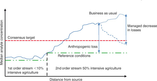
Once estimated, reference conditions should enable substantial gains in managing water quality by accounting for natural variation. The difference between current concentrations of analytes and those likely at reference sites represents the anthropogenic contribution. However, only a portion of this contribution will be manageable (Fig. 9). Recognising that reference conditions vary spatially helps to avoid setting limits that are too high and produce little benefit for environmental values, or are so low that they are impossible to meet. Such limits could be set relative to reference conditions on a concentration basis or, if sufficient flow data is available, on a load basis (Sheeder and Evans 2004).
|
Research over the past three decades has revealed many of the edaphic (i.e. soil and climatic) factors and management (e.g. the placement and timing of P inputs) practices that result in water quality deterioration (e.g. McDowell et al. 2011). We contest that with this knowledge it should now be possible to determine the manageable loss and set a catchment target following an assessment of how low (on the contamination scale) it is possible to go with current mitigation technologies viz. better management of land in percentage of intensive agriculture.
Conclusions
Within the limits of the available data, median values for water quality analytes under reference conditions for streams and rivers are able to be estimated as classified by climate, topography and geology within the River Environment Classification. Confidence in the accuracy of our reference condition estimates over an ANCOVA approach is provided by the fact that more sites classified as minimally disturbed sites (i.e. <5% intensive agricultural land cover) were generally within the confidence limits for each estimate. The establishment of reference condition estimates enabled us to identify those classes with high anthropogenic input and the analytes that are have high levels of enrichment relative to reference conditions within a REC class. Use of the REC also enabled us to account for natural variation in reference conditions and also informed the setting of water quality objectives by avoiding limits or targets that are either too restrictive, and impossible to meet (e.g. if below reference conditions), or so high that they have little ecological effect. It is recommended that this approach be considered by regulatory authorities during the process of setting water quality objectives and limits.
Acknowledgements
This paper has benefited from several discussions within staff from NIWA, AgResearch and Regional Councils and the efforts of the editor and two anonymous reviewers. The work was supported by funded by central government (e.g. Ministry for Science and Innovation contract C10X1006 – Clean Water, Productive Land, and Ministry for the Environment) and data provided by Regional Councils.
References
ANZECC (2000). ‘Australian and New Zealand Guidelines for Fresh and Marine Water Quality’. Vol. 1 and 2. (Australian and New Zealand Environment and Conservation Council and Agriculture and Resource Management Council of Australia and New Zealand: Canberra.)Ballantine, D. J., and Davies-Colley, R. J. (2009) Water quality trends at National River Water Quality Network sites for 1989–2007. Ministry for the Environment, NIWA Client Report HAM2009–026, National Institute of Water and Atmospheric Research, Hamilton, New Zealand. Available from: http://www.mfe.govt.nz/publications/water/
Ballantine, D., Booker, D., Unwin, M., and Snelder, T. (2010). Analysis of national river water quality data for the period 1998–2007. National Institute of Water and Atmospheric Research, Christchurch, New Zealand. Available from: http://www.mfe.govt.nz/publications/water/
Biggs, B. J. F., Duncan, M. J., Jowett, I. G., Quinn, J. M., Hickey, C. W., Davies-Colley, R. J., and Close, M. E. (1990). Ecological characterisation, classification, and modelling of New Zealand rivers: an introduction and synthesis. New Zealand Journal of Marine and Freshwater Research 24, 277–304.
| Ecological characterisation, classification, and modelling of New Zealand rivers: an introduction and synthesis.Crossref | GoogleScholarGoogle Scholar |
Booker, D. J., and Snelder, T. H. (2012). Comparing methods for estimating flow duration curves at ungauged sites. Journal of Hydrology 434–435, 78–94.
| Comparing methods for estimating flow duration curves at ungauged sites.Crossref | GoogleScholarGoogle Scholar |
Chambers, P. A., McGoldrick, D. J., Brua, R. B., Vis, C., Culp, J. M., and Benoy, G. A. (2012). Development of environmental thresholds for nitrogen and phosphorus in streams. Journal of Environmental Quality 41, 1–6.
| Development of environmental thresholds for nitrogen and phosphorus in streams.Crossref | GoogleScholarGoogle Scholar | 1:CAS:528:DC%2BC38XovFSjuw%3D%3D&md5=036bafc9a978ed41a3a156d5f20c468aCAS | 22218168PubMed |
Cooper, A. B., and Thomsen, C. E. (1988). Nitrogen and phosphorus in streamwaters from adjacent pasture, pine and native forest catchments. New Zealand Journal of Marine and Freshwater Research 22, 279–291.
| Nitrogen and phosphorus in streamwaters from adjacent pasture, pine and native forest catchments.Crossref | GoogleScholarGoogle Scholar | 1:CAS:528:DyaL1MXot1Skuw%3D%3D&md5=7ac786b7442a0cffa92c64cedc62b2e8CAS |
De Pauw, N., and Roels, D. (1988). Relationship between biological and chemical indicators of surface water quality. Verhandlungen - Internationale Vereinigung für Theoretische und Angewandte Limnologie 23, 1553–1558.
| 1:CAS:528:DyaL1MXksVCru78%3D&md5=a3f56014eb7da28e497a3b06abfc23efCAS |
Dillon, P. J., and Kirchner, W. B. (1975). The effects of geology and land use on the export of phosphorus from watersheds. Water Research 9, 135–148.
| The effects of geology and land use on the export of phosphorus from watersheds.Crossref | GoogleScholarGoogle Scholar | 1:CAS:528:DyaE2MXhtFGruro%3D&md5=66c8090489f1a270bceb519a9e7d4979CAS |
Dodds, W. K., and Oakes, R. M. (2004). A technique for establishing reference nutrient concentrations across watersheds affected by humans. Limnology and Oceanography, Methods 2, 333–341.
| A technique for establishing reference nutrient concentrations across watersheds affected by humans.Crossref | GoogleScholarGoogle Scholar |
Dodds, W. K., and Welch, E. B. (2000). Establishing nutrient criteria in streams. Journal of the North American Benthological Society 19, 186–196.
| Establishing nutrient criteria in streams.Crossref | GoogleScholarGoogle Scholar |
Dymond, J. R., Ausseil, A.-G., Shepherd, J. D., and Buettner, L. (2006). Validation of a region-wide model of landslide susceptibility in the Manawatu-Wanganui region of New Zealand. Geomorphology 74, 70–79.
| Validation of a region-wide model of landslide susceptibility in the Manawatu-Wanganui region of New Zealand.Crossref | GoogleScholarGoogle Scholar |
GenStat Committee (2010) Genstat v12.2, VSN International. Available from: http://www.vsni.co.uk/downloads/genstat/12th-edition-upgrade (Accessed January 2012).
Hawkins, C. P., Olson, J. R., and Hill, R. A. (2010). The reference condition: predicting benchmarks for ecological and water-quality assessments. Journal of the North American Benthological Society 29, 312–343.
Herlihy, A. T., and Sifneos, J. C. (2008). Developing nutrient criteria and classification schemes for wadeable streams in the conterminous US. Journal of the North American Benthological Society 27, 932–948.
| Developing nutrient criteria and classification schemes for wadeable streams in the conterminous US.Crossref | GoogleScholarGoogle Scholar |
Larned, S. T., Scarsbrook, M. R., Snelder, T. H., and Norton, N. (2003) Nationwide and regional state and trends in river water quality 1996–2002. Ministry for the Environment, NIWA Client Report: CHC2003–051, National Institute of Water and Atmospheric Research, Christchurch, New Zealand.
Lewis, W. M., Melack, J. M., McDowell, W. H., McClain, M., and Richey, J. E. (1999). Nitrogen yields from undisturbed watersheds in the Americas. Biogeochemistry 46, 149–162.
| Nitrogen yields from undisturbed watersheds in the Americas.Crossref | GoogleScholarGoogle Scholar | 1:CAS:528:DyaK1MXlslSlsro%3D&md5=3e621d020ccebff425d1e0b728f9840fCAS |
McDowell, R. W., Larned, S. T., and Houlbrooke, D. J. (2009). Nitrogen and phosphorus in New Zealand streams and rivers: control and impact of eutrophication and the influence of land management. New Zealand Journal of Marine and Freshwater Research 43, 985–995.
| Nitrogen and phosphorus in New Zealand streams and rivers: control and impact of eutrophication and the influence of land management.Crossref | GoogleScholarGoogle Scholar | 1:CAS:528:DC%2BC3cXkvFKrsA%3D%3D&md5=f0f9814785b20556e1fdffbebff05880CAS |
McDowell, R. W., Snelder, T., Littlejohn, R., Hickey, M., Cox, N., and Booker, D. J. (2011). State and potential management to improve water quality in an agricultural catchment relative to a natural baseline. Agriculture, Ecosystems & Environment 144, 188–200.
| State and potential management to improve water quality in an agricultural catchment relative to a natural baseline.Crossref | GoogleScholarGoogle Scholar | 1:CAS:528:DC%2BC3MXhsFCqsLjL&md5=ca82705591e3cabfaa384bab69b8e67fCAS |
MfE (Ministry for the Environment) (2004). ‘New Zealand Land Cover Database (LCDB2)’.(Ministry for the Environment: Wellington.)
Reynoldson, T. B., Norris, R. H., Resh, V. H., Day, K. E., and Rosenberg, D. M. (1997). The reference conditions: a comparison of multimetric and multivariate approaches to assess water-quality impairment using benthic macroinvertebrates. Journal of the North American Benthological Society 16, 833–852.
| The reference conditions: a comparison of multimetric and multivariate approaches to assess water-quality impairment using benthic macroinvertebrates.Crossref | GoogleScholarGoogle Scholar |
Sánchez-Montoya, M. M., Arce, M. I., Vidal-Abarca, M. R., Suárez, M. L., Prat, N., and Gómez, R. (2012). Establishing physio-chemical reference conditions in Mediterranean streams according to the European Water Framework Directive. Water Research 46, 2257–2269.
| Establishing physio-chemical reference conditions in Mediterranean streams according to the European Water Framework Directive.Crossref | GoogleScholarGoogle Scholar |
Scarsbrook, M. R., McBride, C. G., McBride, G. B., and Bryers, G. (2003). Effects of climate variability on rivers: consequences for long term water quality analysis. Journal of the American Water Resources Association 39, 1435–1447.
| Effects of climate variability on rivers: consequences for long term water quality analysis.Crossref | GoogleScholarGoogle Scholar | 1:CAS:528:DC%2BD2cXht1Whur8%3D&md5=40ae830b890c6714de3575947efd8301CAS |
Sheeder, S. A., and Evans, B. M. (2004). Estimating nutrient and sediment threshold criteria for biological impairment in Pennsylvania watersheds. Journal of the American Water Resources Association 40, 881–888.
| Estimating nutrient and sediment threshold criteria for biological impairment in Pennsylvania watersheds.Crossref | GoogleScholarGoogle Scholar | 1:CAS:528:DC%2BD2cXnvFWlu7w%3D&md5=2661bf36d5760c480afb1c81e3761192CAS |
Smith, D. G., and McBride, G. B. (1990). New Zealand’s National Water Quality Monitoring Network- design and first year’s operation. Water Resources Bulletin 26, 767–775.
| New Zealand’s National Water Quality Monitoring Network- design and first year’s operation.Crossref | GoogleScholarGoogle Scholar | 1:CAS:528:DyaK38XksFyjtA%3D%3D&md5=a237051d0cbe682020ceff9a0ffaac37CAS |
Snelder, T. H., and Biggs, B. J. F. (2002). Multi-scale river environment classification for water resources management. Journal of the American Water Resources Association 38, 1225–1240.
| Multi-scale river environment classification for water resources management.Crossref | GoogleScholarGoogle Scholar |
Snelder, T. H., Weatherhead, M., and Biggs, B. J. F. (2004a). Nutrient concentration criteria and characterization of patterns in trophic state for rivers in heterogeneous landscapes. Journal of the American Water Resources Association 40, 1–13.
| Nutrient concentration criteria and characterization of patterns in trophic state for rivers in heterogeneous landscapes.Crossref | GoogleScholarGoogle Scholar | 1:CAS:528:DC%2BD2cXjtFCgsL4%3D&md5=6445e7ce956806cb1defb15d97c3856aCAS |
Snelder, T., Cattanéo, F., Suren, A. M., and Biggs, B. J. F. (2004b). Is the River Environment Classification an improved landscape-scale classification of rivers? Journal of the North American Benthological Society 23, 580–598.
| Is the River Environment Classification an improved landscape-scale classification of rivers?Crossref | GoogleScholarGoogle Scholar |
Snelder, T. H., Woods, R., and Biggs, B. J. F. (2005). Improved eco-hydrological classification of rivers. River Research and Applications 21, 609–628.
| Improved eco-hydrological classification of rivers.Crossref | GoogleScholarGoogle Scholar |
Soranno, P. A., Wagner, T., Martin, S. L., McLean, C., Novitski, L. N., Provence, C. D., and Rober, A. R. (2011). Quantifying regional reference conditions for freshwater ecosystem management: A comparison of approaches and future research needs. Lake and Reservoir Management 27, 138–148.
| Quantifying regional reference conditions for freshwater ecosystem management: A comparison of approaches and future research needs.Crossref | GoogleScholarGoogle Scholar |
Stoddard, J. L., Larsen, D. P., Hawkins, C. P., Johnson, R. K., and Norris, R. H. (2006). Setting expectations for the ecological condition of stream: the concept of reference condition. Ecological Applications 16, 1267–1276.
| Setting expectations for the ecological condition of stream: the concept of reference condition.Crossref | GoogleScholarGoogle Scholar | 16937796PubMed |
Suplee, M. W., Varghese, A., and Cleland, J. (2007). Developing nutrient criteria for streams: an evaluation of the frequency distribution method. Journal of the American Water Resources Association 43, 453–472.
| Developing nutrient criteria for streams: an evaluation of the frequency distribution method.Crossref | GoogleScholarGoogle Scholar | 1:CAS:528:DC%2BD2sXkvFenu7g%3D&md5=d43d764eae8280079a6f2bfff450445bCAS |
Unwin, M., Snelder, T., Booker, D., Ballantine, D., and Lessard, J. (2010). Predicting water quality in New Zealand rivers from catchment-scale physical, hydrological and land cover descriptors using random forest models. Ministry for the Environment, NIWA Client Report: CHC2010–0, National Institute of Water and Atmospheric Research, Christchurch, New Zealand.
USEPA [United States Environmental Protection Agency] (1998). ‘Level III Ecoregions of the Continental United States’ (revision of Omerick 1987). (US Environmental Protection Agency, Washington DC.)
Vant, B., and Huser, B. (2000). Effects of intensifying land-use on the water quality of Lake Taupo. Proceedings of the New Zealand Society of Animal Production 60, 261–264.
Verbyla, A. P., Cullis, B. R., Kenward, M. G., and Welham, S. J. (1999). The analysis of designed experiments and longitudinal data using smoothing splines. Journal of the Royal Statistical Society. Series C, Applied Statistics 48, 269–311.
| The analysis of designed experiments and longitudinal data using smoothing splines.Crossref | GoogleScholarGoogle Scholar |