

Quantifying merging fire behaviour phenomena using unmanned aerial vehicle technology
Alexander Filkov A B C , Brett Cirulis A and Trent Penman A
A School of Ecosystem and Forest Sciences, University of Melbourne, Creswick, Vic. 3363, Australia.
B Bushfire and Natural Hazards Cooperative Research Centre, Melbourne, Vic. 3002, Australia.
C Corresponding author. Email: alexander.filkov@unimelb.edu.au
International Journal of Wildland Fire 30(3) 197-214 https://doi.org/10.1071/WF20088
Submitted: 10 June 2020 Accepted: 20 November 2020 Published: 10 December 2020
Journal Compilation © IAWF 2021 Open Access CC BY
Abstract
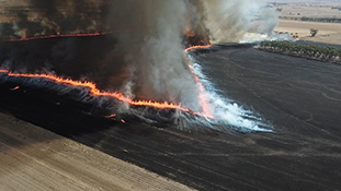
Catastrophic wildfires are often a result of dynamic fire behaviours. They can cause rapid escalation of fire behaviour, increasing the danger to ground-based emergency personnel. To date, few studies have characterised merging fire behaviours outside the laboratory. The aim of this study was to develop a simple, fast and accurate method to track fire front propagation using emerging technologies to quantify merging fire behaviour at the field scale. Medium-scale field experiments were conducted during April 2019 on harvested wheat fields in western Victoria, Australia. An unmanned aerial vehicle was used to capture high-definition video imagery of fire propagation. Twenty-one junction and five inward parallel fire fronts were identified during the experiments. The rate of spread (ROS) of junction fire fronts was found to be at least 60% higher than head fire fronts. Thirty-eight per cent of junction fire fronts had increased ROS at the final stage of the merging process. Furthermore, the angle between two junction fire fronts did not change significantly in time for initial angles of 4–14°. All these results contrast with previous published work. Further investigation is required to explain the results as the relationship between fuel load, wind speed and scale is not known.
Keywords: automatic georeferencing, fast post-processing, field experiments, fire front propagation and tracking, merging fire fronts, operational and management application, remote measurements, UAV.
Introduction
Extreme fire events (EFEs) (Tedim et al. 2018) have become more regular around the world. During the 2019–20 fire season, EFEs in Australia burnt almost 19 million ha, destroyed over 3000 houses, killed 33 people and were estimated to have killed more than 1 billion animals (Filkov et al. 2020b). EFEs create disproportionate risks to environmental and human assets as they can result in many casualties and loss of property. In most cases, these consequences are a result of dynamic fire behaviours (Viegas 2012; Filkov et al. 2018; Tedim et al. 2018; Filkov et al. 2020a).
One dynamic fire behaviour is merging fires (Viegas et al. 2012; Viegas et al. 2013; Thomas et al. 2017; Hilton et al. 2018; Raposo et al. 2018), which can lead to rapid increases in fire intensity and spread rate (Hilton et al. 2017). The convergence of separate individual fires into larger fires is known as coalescence and the merging of two lines of fire intersecting at an oblique angle is termed junction fire or junction fire fronts (Viegas et al. 2012). Fire coalescence, inward parallel fire fronts and junction fire fronts are all examples of merging fire fronts (Fig. 1). Fire coalescence and junction fire fronts behave in a manner that can defy suppression efforts even in the most prepared and equipped regions (Williams and Hamilton 2005). Erratic behaviour and difficulties in suppression allow fires to burn more intensely over larger areas, increasing the likelihood of loss of life, property and other assets.
|
Merging fire fronts have been recorded in several significant bushfires. For example, in the 2003 Canberra fires, the McIntyre’s Hut and Bendora fires merged in the early afternoon (Doogan 2006). The merging fire apex P (Fig. 1b) spread rapidly and developed into an extremely destructive junction fire that resulted in four deaths, many injuries and property losses valued at AU$600 million to AU$1 billion.
Junction fire fronts have generally been studied experimentally at the metre scale (Viegas et al. 2012; Viegas et al. 2013; Raposo et al. 2018; Sullivan et al. 2019) with only one exception (Raposo et al. 2018), where the authors conducted three field experiments (47, 52 and 75 m). During laboratory and field experiments, researchers varied the angle between two fire fronts (θ) (Viegas et al. 2012), slope of the fuel bed, fuel type (Viegas et al. 2013; Raposo et al. 2018) and wind conditions (Sullivan et al. 2019).
There is a strong relationship between the velocity of the intersect point and the angle between the fire lines (Viegas et al. 2012). The non-dimensional form of the rate of spread R′ of the intersect point of two oblique fire fronts (junction fire fronts) appears in Eqn 1 (Viegas et al. 2012).
RP is the rate of spread of the intersect point of two junction fire fronts; R0 is the basic rate of spread of a linear fire front in the same fuel bed in no-wind and no-slope conditions.
Two stages of junction fire development have been identified (Viegas et al. 2013; Raposo et al. 2018): an acceleration phase where the apex rate of spread (RP) greatly increases at the start of the fire and a deceleration phase where the apex slows down and the fire extinguishes. In the deceleration phase, the fire behaves like a linear fire front. Viegas et al. (2013) argued that slope increases the distance travelled by the intersect point in the acceleration phase and changes in fuel bed composition have no effect on the non-dimensional rate of spread R′.
Fires may be classified as buoyancy-dominated or wind-dominated (Morvan and Frangieh 2018). Typically, buoyancy-driven fires are thought to propagate largely by radiation because most of the hot gases move upwards, and wind-driven fires largely by convection because the hot gases are pushed forward (Morvan and Frangieh 2018). Sullivan et al. (2019) conducted a series of 1-m-scale experiments in the absence and presence of wind to study its influence on apex velocity. In their study, they developed and introduced the so-called null hypothesis (Eqn 2):
where θ is the angle between junction fire fronts and Rl is the rate of spread of the linear fire front. They proposed an original approach to obtain the basic rate of spread R0 for windy conditions. It was calculated as the rate of spread of the linear fire front (ignition line) Rl perpendicular to the wind and corrected to compensate for the effect of the different junction angles on each R0. This was done by multiplying the rate of spread of the linear fire front Rl by the sine of half of each angle between junction fire fronts (Eqn 2).
This hypothesis assumes junction fire fronts merge under quasi-steady conditions and is a reasonable null hypothesis for no-wind conditions. Other researchers found no evidence that R′ was enhanced over the null hypothesis for no-wind conditions, but found increases in R′ for wind-driven conditions (Viegas et al. 2012, 2013; Raposo et al. 2018). This discrepancy was attributed to the different scale of the experiments, fuel load and fuel type (dense eucalyptus litter), and possibly fuel configuration that permitted a fire upstream of the ignition line. However, the mechanisms of heat transfer were not measured or analysed in any of these studies.
Physics-based modelling can be a powerful instrument to uncover physical phenomena beyond experimental limitations. Recently, Thomas et al. (2017) tested similar junction angles θ to Viegas et al. (2012) using the coupled atmosphere–fire model WRF-Fire (Coen et al. 2013), but at a larger scale: each simulated fire line was 1000 m long. They found that, in addition to the bulk fire-induced surface flow, sets of counter-rotating pairs of vertical vortices lying on or ahead of the fire lines of the junction fires were formed, and these vortices produced local acceleration of the fire front. However, they concluded that the vortical structures were not well resolved at the 20-m resolution used and were likely too small to be properly resolved by their simulations. Thomas et al. (2017) found some quantitative differences in the acceleration of the apex with the results of Viegas et al. (2012). The lack of agreement could be attributed to a scaling problem. For instance, laboratory experiments for low angles of junction fire fronts cannot capture all effects due to the small scale (Raposo et al. 2018).
Although physics-based models are the best instrument to provide insights into different phenomena, they are too slow and complex for operational purposes. Analytical and simplified models take seconds to minutes to produce a prediction including basic wind effects, compared with hours to days for a full physical model (Frangieh et al. 2018). The first simple analytical model based on energy concentration between the two arms of the junction was proposed by Viegas et al. (2012). It had considerable limitations, such as no slope or wind gradients. Hilton et al. (2018) developed a simplified model of the wind fields around wildfires based on a two-dimensional ‘pyrogenic’ potential flow formulation. When coupled to a wildfire perimeter propagation model, this can replicate basic wildfire interaction effects including fire line attraction, the shape of fire fronts and the enhanced coalescence of spot fires (Hilton et al. 2017). However, the model assumes that the plume is not significantly affected by the wind. It is therefore likely that the model can only be applied under certain conditions and further work is needed to explore the experimental parameter space and extend the model for wind-driven conditions. The authors concluded that despite the good match to experimental results, the model should take flame attachment into account and it is likely that the model only applies under certain conditions that have not been fully explored in the experimental parameter space.
Extensive high temporal and spatial resolution experimental data at larger scales are required to fully understand how a given fire will merge and spread. Unmanned aerial vehicles (UAVs or drones) may be a useful tool in obtaining these measurements. In the last decade, they have been well utilised in the study of wildfires (Merino et al. 2012; Hua and Shao 2017; Fernández-Guisuraga et al. 2018). UAVs have been used for fire detection and monitoring (Hua and Shao 2017; Moran et al. 2019), fire management (Merino et al. 2012) and post-fire monitoring (Fernández-Guisuraga et al. 2018). They can be equipped with various sensing instruments, ranging from optical sensors (including visible and infrared) to microwave sensors (radar and LiDAR). Owing to flexibility, low cost and high-resolution data collection, rotary-wing drone remote sensing can fill data gaps about different fire behaviour phenomena.
The aims of the present study were:
to develop a simple, fast and accurate method to track fire front propagation using UAVs,
to quantitatively characterise fire behaviour of merging fires, and
to compare fire behaviour characteristics with previous studies.
Methods
Study area and equipment
The study was conducted on agricultural lands in western Victoria, Australia (Fig. 2a). Small- and medium-scale field experiments were conducted between 1503 and 1620 hours on 12 April 2019 near Kingston, 110 km west of Melbourne. Two harvested wheat fields were used as experimental plots, as they form fairly homogeneous fuel beds. Fuel height varied from 18 to 30 cm in each plot and fuel load and moisture content were 1.1 ± 0.15 tonnes ha−1 (t ha−1) (0.11 kg m−2) and 11.9 ± 2% respectively. Fuel (straw) bed density and surface area-to-volume ratio were 0.46 ± 0.08 kg m−3 and 2240 ± 185 m−1 respectively. A drip torch (50% diesel fuel to 50% petrol) was used to progressively ignite lines of fuel in parallel, starting at the downwind edge of the plot (Fig. 2b). For each plot, the downwind line was ignited first, IL1 or IL4 respectively, and allowed to fully spread downwind to a fuel break and self-extinguish. Then, the next ignition line in the upwind direction (IL2 or IL5) was ignited and allowed to spread and self-extinguish. Finally, the last ignition line on the plot was ignited (IL3 or IL6). A total of six straight ignition lines (IL1–IL6) between 400 and 480 m long were ignited during the experiment.
|
An automatic weather station (AWS, 30-min temporal resolution) and two 2-dimensional DS-2 sonic sensors (Decagon Devices, Inc.) were used for air temperature, relative humidity, wind direction and speed measurements. The Ballarat Aerodrome AWS (no. 89002) is located 21 km south-east from the plots (−37.5127, 143.7911). Locations of the sonic sensors are shown on Fig. 2b. One sonic sensor (Sonic 1, Fig. 2b) was repositioned during the study based on ignition location. Another sensor (Sonic 2) was used as a control sensor and remained in the same location during all tests. Air temperature and relative humidity were 20.5 ± 0.3°C and 22.8 ± 2% respectively. Wind direction data were taken from the AWS owing to the direction component of the sonic sensors malfunctioning. Wind direction (direction from which wind originates) was northerly at the beginning of the experiment, switching to north–north-westerly at the end. Wind speed was measured every minute 1.5 m above ground and was in the range 1.8–7.0 m s−1 (Fig. 3) with an average speed of 3.6 and 4.7 m s−1 for Sonic 1 and 2 respectively. It was not possible to analyse the influence of wind on merging fires owing to short duration of the merging process (less than 1 min) and coarse temporal resolution (1 min) of the sonic sensors. The slope was less than 5° at all plots.
|
A DJI Mavic Pro UAV was used to capture high-definition video imagery of fire propagation in synchrony with sensor data from the on-board global positioning system (GPS) and inertial measurement unit (IMU). These sensors enabled the platform/camera orientation and position in space to be aligned with the video footage and the fire propagation georeferenced in GIS (geographic information system) software.
Data capture and processing
Video data were captured using the onboard camera on the DJI Mavic Pro. To minimise the georeferencing error of the final imagery, a stationary flight with an altitude of 30 m and a 90° camera angle (looking straight down) was maintained for each junction fire while video footage was recorded. Video was recorded at 1080p (1920 × 1080 pixels) resolution at 60 frames per second (fps). The CIRRUAS application (CompassDrone, Denver, CO, USA) was used with an android phone to record the necessary flight metadata for post processing. For each video footage, a CSV file was produced with the following metadata: UNIX time stamp, platform heading angle, platform pitch angle, platform roll angle, sensor latitude, sensor longitude, sensor true altitude, sensor horizontal field of view, sensor vertical field of view, sensor relative azimuth angle, sensor relative elevation angle, sensor relative roll angle. The post-processing phase was completed for each video and metadata files using the Full Motion Video (FMV) toolbox (Fig. 4a) within the ArcGIS Pro software (Macdonald 2017).

|
The video file was converted into an FMV-compliant format (georeferenced) before analysing the video footage. The metadata file containing sensor information is combined with the video file in a process called Multiplexing (Fig. 4b). The result is a video file with each frame georeferenced (Fig. 5, bottom window). Once it is multiplexed, the georeferenced frame of the filmed area appears on the map (Fig. 5, top window). The frame had a trapezium shape with dimensions of 100 m (top) × 110 m (base) × 60 m (sides). The multiplexed video file was then used to identify and spatially define fire fronts at set time intervals. The process of multiplexing takes ~3 min for each minute of video (Intel i7 CPU, 32 Gb RAM).

|
After the ignition line was started, the fire front produced fire tongues (Fig. 5, bottom window). Fire lines of two neighbouring tongues naturally merged together were identified as junction fire fronts and the angle between them as the initial angle. Parallel fire fronts were identified as two fire tongues burning parallel to each other.
We measured the travelling distance of the intersect point P (Fig. 1b) every 2 s to calculate rate of spread (ROS) of junction fire fronts. To calculate the angle between junction fire fronts, we used the law of cosines θ = arccos ((c2 + b2 – a2)/2bc), where a, b and c are the sides of the triangle. To use this formula, we measured the length of all three sides of the triangle. Junction fire front lengths were determined as sides b and c of the triangle (Fig. 1b). Three points on the fire fronts were selected for each time step in the FMV toolbox using the Add graphics tool (Fig. 6a). One point was an intersect of two junction fire fronts (intersect point P) and two others were the points on each fire line. Once a point is selected, it automatically appears on the ArcGIS Pro map (Fig. 6b). The Save video graphics tool was then used to save created points in the ArcGIS Pro project. For better representation of fire progression, the selected points and merging fire lines were highlighted with different colours. Using the ArcGIS Pro Measure tool, the distance between selected points and the travelling distance of the intersect point were measured. Measurements of the sides of the triangle (a, b, c) and the travelling distance of intersect point P for each time step of 21 junction fires took ~3 h.
|
All parallel fire fronts observed during the experiments were approaching each other (i.e. inward parallel fire fronts). One point was selected on each fire front (left and right fire fronts hereafter) along the same convergence plane. After 5 s of spread, a second point was placed on each fire front and the distance between point pairs was measured. ROS could then be calculated for each fire front, left and right.
The non-dimensional form of the rate of spread R′ described in Eqn 2 was used to compare ROS between different phenomena and with other studies. All the experiments were conducted in windy conditions. As such, it is important to describe the approach used to determine the basic ROS in our work. First, we determined the ROS of the linear fire front Rl – the ROS of the closest head fire to junction or parallel fire fronts. Basic ROS R0 was then calculated following the method used by Sullivan et al. (2019), where the ROS of the linear fire front is corrected to compensate for the effect of the different oblique angles on R0 (R0 = Rlsin(θ/2)). The angle between the linear fire front and wind direction varied in the range 35–80°.
The ROS of the linear fire front Rl was measured in the vicinity of each junction and parallel fire fronts every 2 and 5 s respectively for their entire duration. Different time intervals were chosen owing to the significant difference in duration of selected phenomena. Ambient wind conditions were similar for each pair of linear fire front and junction fire front, linear fire front and parallel fire front as they were at close proximity to each other and measured at the same time.
All measurements were done in the area surrounded by the trapezium frame with the longest base of 110 m (Fig. 5) and after 30 s from ignition to avoid the build-up phase influencing the results (Cheney and Gould 1997). A head fire takes time to reach equilibrium or steady-state ROS after ignition; this process has been referred as the fire growth or build-up (Cheney and Gould 1997). Cheney et al. (1993) found that line fires in grasslands appeared to reach a quasi-steady speed across small plots (100 × 100 m) after ~15 s for ignition lines that were nominally 50 m long.
A linear regression analysis was conducted for quantitative estimations. Specifically, we calculated the slope of the regression line m, adjusted R2 and significance value P. Response variables were the ROS of the intersect point of two junction fire fronts RP and the angle θ between junction fire fronts. The predictor variable was time. Negative and positive relationships are indicated as decreasing and increasing trends (slopes) respectively. Owing to the different duration of each merging fire, we converted time steps to percentages of the final time. Initial time is the time when two fire tongues naturally merged together. Final time for RP is the last time the angle between junction fire fronts became 180°. The final time for θ is one timestep prior to the last time.
In order to test the hypothesis that the ROS of merging fire fronts is statistically different from linear fire fronts, a one-way ANOVA was performed. Parallel fire fronts were excluded from the analysis as the assumption of homogeneity was not satisfied and the group sizes were not equal. Prior to conducting the ANOVA, the assumption of normality was evaluated using a Shapiro–Wilk test at the 0.05 level and was determined to be satisfied as the junction and linear fire fronts P values were 0.07 and 0.56 respectively. Furthermore, the assumption of homogeneity of variances was tested and satisfied based on Lavene’s F test (F = 3.35, P = 0.07).
Results
Eleven videos were filmed during experiments and post processed (Fig. 7a). Twenty-six merging fire fronts were identified: 21 junction fire fronts and 5 parallel fire fronts (Fig. 7b) (Appendix 1, Tables A1–A4).

|
The junction fire fronts identified were separated into four groups depending on the recorded initial angle between oblique fire fronts θin: 4–14°, 28–34°, 40–59° and 77°. The highest number of fires (43%) were observed in the 28–34° group.
The ROS of junction, linear and parallel fire fronts was calculated as an average of all 2- and 5-s time intervals (Fig. 8). The mean ROS of junction fire fronts (1.75 m s−1, s.d. 0.66) was 1.6 times higher than for linear (1.11 m s−1, s.d. 0.34) and at least 20 times higher than for parallel (0.08 m s−1, s.d. 0.05) fire fronts. Acute-angle (<14°) ROS of junction fire fronts was greater by 3–6 times than the linear fire front ROS. The independent between-groups ANOVA indicated that the mean ROS for the junction fire fronts was significantly different than the linear fire fronts, F = 18.36, P = 9.8 × 10⁻⁵. Thus, the null hypothesis of no differences between the means was rejected.
|
Comparisons of ROS and the angle between junction fire fronts θ are presented on Figs 9 and 10. ROS increased as the initial angle decreased (Fig. 9). The mean ROS was 1.02 m s−1 (s.d. 0.19), 1.49 m s−1 (s.d. 0.65), 1.49 m s−1 (s.d. 0.44) and 3.44 m s−1 (s.d. 1.81) for the initial angles 77°, 40–59°, 28–34° and 4–14° respectively. We found 38% of junction fire fronts exhibited an increase in ROS at the final stage of the merging process. Linear regression analysis showed that at the 0.05 level, the slope is not significantly different from zero for all initial angles (Fig. 9). This suggests that junction fire fronts do not notably change ROS during the merging process. However, this suggestion requires further investigation as the dataset is limited.
|
|
The angle between fire fronts did not increase significantly over time (m = 0.05, P = 0.228) (Fig. 10) for two oblique fire fronts with initial angles (θin) 4–14°. However, for the initial angles 28–34°, 40–59° and 77°, the slope of the regression line was between 0.3 and 0.4 and was statistically significant (P < 0.035).
Mean ROS of parallel fire fronts was 0.07 m s−1, varying between 0.001 and 0.33 m s−1 (Fig. 11). ROS increases as fire lines come closer to each other. Faster ROS of the right fire line was observed during the experiments. It can be assumed that because the developed parallel fire fronts were not perfectly aligned with the wind direction (not possible in the field experiments), the resulting ROS was different for the left and right fire lines. It is supposed that small fluctuations of the ROS related to change in the wind speed (Fig. 3) rather than fire itself.
|
The ROS of the linear fire fronts Rl did not change considerably during the lifetime of the merging fires and did not influence merging fire front development (Fig. 12). Standard deviation of Rl varied in the range 0.04–0.55 m s−1.
|
Fig. 13 shows comparison of our results with studies of Sullivan et al. (2019), Viegas et al. (2012) and Thomas et al. (2017). Comparison with the null hypothesis (Eqn 2) and laboratory results of Sullivan et al. (2019) (Fig. 13a) showed that the non-dimensionless ROS R′ in our experiments was greater and smaller than the null hypothesis (in contrast to Sullivan et al. (2019)) cosec(θ/2).
|
For comparison with the simplified analytical model of Viegas et al. (2012), we modelled our data with the Belehradek model (Ross 1993) (Fig. 13b). Non-linear regression with the Levenberg–Marquardt algorithm (Ranganathan 2004) was used (adj. R2 = 0.92):

Similarly to Sullivan et al. (2019), we did not get agreement with Viegas et al. (2012). Although Viegas et al. (2012) conducted experiments in no-wind conditions, the R′ in their study was higher than that observed in our results (Fig. 13b) and those of Sullivan et al. (2019) (Fig. 13a).
Comparison of dimension ROS (RP) with the numerical simulation of Thomas et al. (2017) shows good agreement (Fig. 13c) despite different fuel types and loads.
Discussion and conclusions
The ROS of junction fire fronts is significantly different and higher than linear fire front ROS, which is consistent with other studies (Viegas et al. 2012, 2013; Sullivan et al. 2019). A greater than 60% increase in ROS was observed for junction fire fronts. However, the ROS of junction fire fronts did not change notably during the merging process (Fig. 9), in contrast to Viegas et al. (2012), Raposo et al. (2018), Thomas et al. (2017) and Sullivan et al. (2019). Previous studies (Viegas et al. 2013; Raposo et al. 2018) identified an initial acceleration phase followed by a deceleration phase for each junction fire development (Viegas et al. 2013; Raposo et al. 2018); however, our results did not show these pronounced phases for each junction fire. All fires behaved differently, having either deceleration-only, acceleration-only or both phases for all initial-angle groups. For instance, 38% of junction fire fronts showed an increase in ROS in the final stage of the merging process in contrast to Viegas et al. (2013 and Raposo et al. (2018). It is problematic for drawing any conclusion as the number of junction fires and measurement points for individual fires are limited.
We observed an increase of current angle θ in time for all initial angles (Fig. 10) except 4–14°, despite the fact the ROS of apex P did not change considerably during the merging process. Viegas et al. (2012) found the value of θ increases continuously, regardless of the initial configuration of the fire lines. However, the rate of increase notably differs between our studies. In the study of Viegas et al. (2012), the slope of the linear regression line (rate of change) decreases with increase in initial angle between two oblique fire fronts, namely 0.62, 0.16, 0.07 for 10°, 30° and 45° initial angle respectively. In our study, we observed the opposite effect: for initial angles 14°, 28–34° and 40–59°, the slope was 0.05, 0.3 and 0.3 respectively (Fig. 10). Without high-resolution measurements of radiative and convective heat transfer, it is difficult to determine why a significant increase of the current angle between two oblique fire fronts did not result in a significant decrease of ROS for initial angles above 28°. It should be noted that in field conditions, wind direction and speed are not constant and that resulted in asymmetry for some junction fire fronts. Asymmetry could affect the ROS and merging process in some cases.
Comparison of junction fire fronts with different length of oblique fire fronts showed no notable influence, in contrast to Sullivan et al. (2019) (Fig. 14). Sullivan et al. (2019) conducted junction fire experiments for 0.8- and 1.5-m ignition lines and found that the rates of vertex propagation in the presence of wind were consistently higher and statistically significant for 1.5 m than those for the 0.8-m ignition lines. In our study, similar ROS were observed for different junction fire front lengths (3.6–22 m) and angles. In the experiments of Sullivan et al. (2019), fuel was both within and outside the junction lines, providing fire spread both inward and outward. Such a fuel layout was not observed during field experiments and may be one of the reasons for the discrepancy.
|
Despite different trends in apex acceleration, we obtained similar results to Sullivan et al. (2019) for the mean ROS of junction fire fronts RP. With increase of initial angle of junction fire fronts from 15° to 30°, 45° and 60° in Sullivan et al. (2019), mean ROS for 0.8-m ignition lines decreased 12.8, 37.8 and 37.8% respectively. In our study, increase from 14° to 28–34°and 40–59° resulted in a decrease of mean ROS of 38.2 and 38.2% respectively. We obtained very good qualitative agreement of mean ROS reduction for all angles, except 30°, despite different spatial scales, experiment design and fuel properties.
Analysis of video footage of merging fire fronts revealed that in all cases, junction fire fronts have a different shape to those in previous studies (Fig. 15). Different configurations of ignition lines can result in different ROS of the intersect point RP. It is hypothesised that the left and right shoulder (Fig. 15b) create complex convective structures and cause changes in the ROS. In our experiments, we observed increase of the ROS in almost 40% of junction fire fronts at the final stage of merging in contrast to a decrease or no change in the ROS in previous research (Viegas et al. 2012, 2013; Raposo et al. 2018; Sullivan et al. 2019). This configuration (Fig. 15b) may also prevent an increase of an angle between two fire lines for initial angles smaller than 30° and requires further investigation.
|
Although Sullivan et al. (2019) found that for the wind-driven experiments, there is an increase of the rate of propagation of the vertex above what would be expected from trigonometry alone (Eqn 2), we did not observe such an increase for all junction fire fronts. Our ROS were larger and smaller than the null hypothesis (Eqn 2) even with wind speeds of 1.8–7.0 m s−1. It can be assumed that in field conditions and for wind speeds higher than 1 m s−1, the R′ of junction fire fronts is more complex.
The dimensionless ROS R′ in our study is lower than of Viegas et al. (2012). The difference was up to 373%, with an average of 66% (relative to our data). A potential reason for this discrepancy could be from the way basic ROS was calculated. Viegas et al. (2012) calculated it without wind for a linear fire front using the same experimental conditions. In our study, we measured R0 of the closest linear fire front in windy conditions and then corrected it to compensate for the effect of the different oblique angles. This approach allows comparisons with future experiments in different wind conditions and other studies. A similar approach was used by Sullivan et al. (2019). Even using the value of basic ROS found by Viegas et al. (2012) for straw (0.002 m s−1) gives us values 30-fold higher than in their study.
Thomas et al. (2017) also conducted a comparison of numerical simulations (length of fire lines ~1 km) with the experimental results of Viegas et al. (2012) (length ~8 m). Their results showed no quantitative agreement as well. They assumed that the reason was the different scale of experiments and numerical modelling.
Fuel type and load may be have caused difference in results with Viegas et al. (2012) and Sullivan et al. (2019). Fuel in our study was a harvested wheat crop with a load of 0.11 kg m−2. Viegas et al. (2012) used pine needle litter with a fuel load of 0.6 kg m−2 (six times higher) and Sullivan et al. (2019) used eucalypt forest fuel litter of 1.2 kg m−2 comprising fallen leaves, twigs and bark (10 times higher). Increasing fuel load may result in increase of the ROS owing to a significant effect on the efficiency of heat transfer to unburnt fuel (Plucinski and Anderson 2008). A comparison with the numerical simulation of Thomas et al. (2017) shows good agreement (Fig. 13c) despite the fact that the fuel load in Thomas et al. (2017) was seven times higher and the experiments were conducted in no-wind conditions.
A decrease of fuel moisture content and air relative humidity should increase the ROS (Rossa 2017); however, a limitation of the data is that we cannot estimate these values. Neither Viegas et al. (2012) nor Thomas et al. (2017) mentioned the moisture content of the fuel bed and air relative humidity in their studies. Sullivan et al. (2019) indicated 3–6% fuel moisture content, at least two times lower than in our experiments (11.9%) and 30.7% relative humidity (almost 8% higher than in our experiments).
The quantification of captured video and photo imagery has traditionally been challenging and requires significant pre-experimental set up time or a complex post-processing workflow. The approach used in these experiments has the benefit of minimal set-up time (hours) with the resulting data being highly accurate across space and time. With further development and testing, it shows promise as a valuable tool for fire behaviour research, operational and management applications.
Summary
Several preliminary small- and medium-scale field experiments were conducted on harvested wheat fields to characterise fire behaviour using emerging technologies. A UAV was used to capture high-definition video imagery of fire propagation. Twenty-one junction fire fronts and five inward parallel fire fronts were identified during the experiments. Comparison between the few available studies showed considerable variation in ROS for similar conditions. These raises the following basic questions:
Scaling. Does the size of merging fires change the ROS? The results of Raposo et al. (2018) (7–75 m) and our results (3.6–22 m) demonstrate that junction fire behaviour is similar at all tested scales, whereas Sullivan et al. (2019) showed an increase in the ROS from 0.8 to 1.8 m.
Fuel load and structure. Do the fuel structural properties (bulk density, porosity, surface-to-volume ratio, heterogeneity, etc.) change the ROS of merging fires? We obtained similar ROS to Thomas et al. (2017) (grass, 7× higher fuel load), but much lower ROS than Viegas et al. (2012) (pine needles, 6× higher) and Sullivan et al. (2019) (eucalypt litter, 10× higher).
Wind speed. How does a change in wind speed modify the ROS? We are not aware of any studies.
Experimental design. How realistic is the V-shape contour? Our observations showed that junction fire fronts in the field always have shoulders at the top of the V, which could result in different fire behaviour compared with a ‘classical’ V-shape contour. This may result in acute angles and increased R′ at the final stage of merging.
Existing studies on merging fires are disconnected. Future research needs to conduct experiments with similar initial conditions and measurements of convective and radiative energy. Without such data, it is not possible to draw any conclusion regarding the problems mentioned above. UAVs provide a means of improving data collection for this purpose.
Conflicts of interest
The authors declare no conflicts of interest.
Acknowledgements
This study was funded by the Bushfire and Natural Hazards Cooperative Research Centre ‘Determining threshold conditions for extreme fire behaviour’ project. We thank John McKinnon for providing access to his farmland for the experiments.
References
Cheney N, Gould J (1997) Fire growth and acceleration. International Journal of Wildland Fire 7, 1–5.| Fire growth and acceleration.Crossref | GoogleScholarGoogle Scholar |
Cheney NP, Gould J, Anderson W (1993) The influence of fuel, weather and fire shape variables on fire-spread in grasslands. International Journal of Wildland Fire 3, 31–44.
| The influence of fuel, weather and fire shape variables on fire-spread in grasslands.Crossref | GoogleScholarGoogle Scholar |
Coen JL, Cameron M, Michalakes J, Patton EG, Riggan PJ, Yedinak KM (2013) WRF-Fire: coupled weather–wildland fire modeling with the weather research and forecasting model. Journal of Applied Meteorology and Climatology 52, 16–38.
| WRF-Fire: coupled weather–wildland fire modeling with the weather research and forecasting model.Crossref | GoogleScholarGoogle Scholar |
Doogan M (2006) ‘The Canberra firestorm: inquests and inquiry into four deaths and four fires between 8 and 18 January 2003: Vol. I.’ (ACT Magistrates Court: Canberra, ACT, Australia)
Fernández-Guisuraga JM, Sanz-Ablanedo E, Suárez-Seoane S, Calvo L (2018) Using unmanned aerial vehicles in post-fire vegetation survey campaigns through large and heterogeneous areas: opportunities and challenges. Sensors 18, 586
| Using unmanned aerial vehicles in post-fire vegetation survey campaigns through large and heterogeneous areas: opportunities and challenges.Crossref | GoogleScholarGoogle Scholar |
Filkov AI, Duff TJ, Penman TD (2018) Improving fire behaviour data obtained from wildfires. Forests 9, 81
| Improving fire behaviour data obtained from wildfires.Crossref | GoogleScholarGoogle Scholar |
Filkov AI, Duff TJ, Penman TD (2020a) Frequency of dynamic fire behaviours in Australian forest environments. Fire 3, 1–19.
| Frequency of dynamic fire behaviours in Australian forest environments.Crossref | GoogleScholarGoogle Scholar |
Filkov AI, Ngo T, Matthews S, Telfer S, Penman TD (2020b) Impact of Australia’s catastrophic 2019/20 bushfire season on communities and environment. Retrospective analysis and current trends. Journal of Safety Science and Resilience 1, 44–56.
| Impact of Australia’s catastrophic 2019/20 bushfire season on communities and environment. Retrospective analysis and current trends.Crossref | GoogleScholarGoogle Scholar |
Frangieh N, Morvan D, Meradji S, Accary G, Bessonov O (2018) Numerical simulation of grassland fires behavior using an implicit physical multiphase model. Fire Safety Journal 102, 37–47.
| Numerical simulation of grassland fires behavior using an implicit physical multiphase model.Crossref | GoogleScholarGoogle Scholar |
Hilton J, Sharples J, Sullivan A, Swedosh W (2017) Simulation of spot fire coalescence with dynamic feedback. In ‘MODSIM2017: 22nd International congress on modelling and simulation’, 3–8 December 2017, Hobart, Tas., Australia (Eds G Syme, D Hatton MacDonald, B Fulton, J Piantadosi) pp. 1111–1117. (Modelling and Simulation Society of Australia and New Zealand)
Hilton JE, Sullivan AL, Swedosh W, Sharples J, Thomas C (2018) Incorporating convective feedback in wildfire simulations using pyrogenic potential. Environmental Modelling & Software 107, 12–24.
| Incorporating convective feedback in wildfire simulations using pyrogenic potential.Crossref | GoogleScholarGoogle Scholar |
Hua L, Shao G (2017) The progress of operational forest fire monitoring with infrared remote sensing. Journal of Forestry Research 28, 215–229.
| The progress of operational forest fire monitoring with infrared remote sensing.Crossref | GoogleScholarGoogle Scholar |
Macdonald O (2017) Getting to know ArcGIS Pro. The Cartographic Journal 54, 284–285.
| Getting to know ArcGIS Pro.Crossref | GoogleScholarGoogle Scholar |
Merino L, Caballero F, Martínez-de-Dios JR, Maza I, Ollero A (2012) An unmanned aircraft system for automatic forest fire monitoring and measurement. Journal of Intelligent and Robotic Systems: Theory and Applications 65, 533–548.
| An unmanned aircraft system for automatic forest fire monitoring and measurement.Crossref | GoogleScholarGoogle Scholar |
Moran CJ, Seielstad CA, Cunningham MR, Hoff V, Parsons RA, Queen L, Sauerbrey K, Wallace T (2019) Deriving fire behavior metrics from UAS imagery. Fire 2, 36
| Deriving fire behavior metrics from UAS imagery.Crossref | GoogleScholarGoogle Scholar |
Morvan D, Frangieh N (2018) Wildland fires behaviour: wind effect versus Byram’s convective number and consequences upon the regime of propagation. International Journal of Wildland Fire 27, 636–641.
| Wildland fires behaviour: wind effect versus Byram’s convective number and consequences upon the regime of propagation.Crossref | GoogleScholarGoogle Scholar |
Plucinski MP, Anderson WR (2008) Laboratory determination of factors influencing successful point ignition in the litter layer of shrubland vegetation. International Journal of Wildland Fire 17, 628–637.
| Laboratory determination of factors influencing successful point ignition in the litter layer of shrubland vegetation.Crossref | GoogleScholarGoogle Scholar |
Ranganathan A (2004) The Levenberg–Marquardt algorithm. Available at https://www.academia.edu/660131/The_levenberg_marquardt_algorithm [Verified 27 November 2020]
Raposo JR, Viegas DX, Xie X, Almeida M, Figueiredo AR, Porto L, Sharples J (2018) Analysis of the physical processes associated with junction fires at laboratory and field scales. International Journal of Wildland Fire 27, 52–68.
| Analysis of the physical processes associated with junction fires at laboratory and field scales.Crossref | GoogleScholarGoogle Scholar |
Ross T (1993) Bělehrádek-type models. Journal of Industrial Microbiology 12, 180–189.
| Bělehrádek-type models.Crossref | GoogleScholarGoogle Scholar |
Rossa CG (2017) The effect of fuel moisture content on the spread rate of forest fires in the absence of wind or slope. International Journal of Wildland Fire 26, 24–31.
| The effect of fuel moisture content on the spread rate of forest fires in the absence of wind or slope.Crossref | GoogleScholarGoogle Scholar |
Sullivan AL, Swedosh W, Hurley RJ, Sharples JJ, Hilton JE (2019) Investigation of the effects of interactions of intersecting oblique fire lines with and without wind in a combustion wind tunnel. International Journal of Wildland Fire 28, 704–719.
| Investigation of the effects of interactions of intersecting oblique fire lines with and without wind in a combustion wind tunnel.Crossref | GoogleScholarGoogle Scholar |
Tedim F, Leone V, Amraoui M, Bouillon C, Coughlan RM, Delogu MG, Fernandes MP, Ferreira C, McCaffrey S, McGee KT, Parente J, Paton D, Pereira GM, Ribeiro ML, Viegas DX, Xanthopoulos G (2018) Defining extreme wildfire events: difficulties, challenges, and impacts. Fire 1, 9
| Defining extreme wildfire events: difficulties, challenges, and impacts.Crossref | GoogleScholarGoogle Scholar |
Thomas CM, Sharples JJ, Evans JP (2017) Modelling the dynamic behaviour of junction fires with a coupled atmosphere–fire model. International Journal of Wildland Fire 26, 331–344.
| Modelling the dynamic behaviour of junction fires with a coupled atmosphere–fire model.Crossref | GoogleScholarGoogle Scholar |
Viegas DX (2012) Extreme fire behaviour. In ‘Forest management: technology, practices and impact.’ (Eds ACB Cruz, REG Correia) pp. 1–56 (Nova Science Publishers, Inc.: New York, NY, USA)
Viegas DX, Raposo JR, Davim DA, Rossa CG (2012) Study of the jump fire produced by the interaction of two oblique fire fronts. Part 1. Analytical model and validation with no-slope laboratory experiments. International Journal of Wildland Fire 21, 843–856.
| Study of the jump fire produced by the interaction of two oblique fire fronts. Part 1. Analytical model and validation with no-slope laboratory experiments.Crossref | GoogleScholarGoogle Scholar |
Viegas DX, Raposo J, Figueiredo A (2013) Preliminary analysis of slope and fuel bed effect on jump behavior in forest fires. Procedia Engineering 62, 1032–1039.
| Preliminary analysis of slope and fuel bed effect on jump behavior in forest fires.Crossref | GoogleScholarGoogle Scholar |
Williams J, Hamilton L (2005) The mega-fire phenomenon: toward a more effective management model. A concept paper. Brookings Institution. (Washington, DC, USA) Available at http://www.bushfirecrc.com/sites/default/files/managed/resource/mega-fire_concept_paper_september_20_ 2005.pdf [Verified 9 September 2019]
Appendix 1

|

|

|

|