

An evaluation of empirical and statistically based smoke plume injection height parametrisations used within air quality models
Joseph L. Wilkins A B C G , George Pouliot A , Thomas Pierce A , Amber Soja D E , Hyundeok Choi D E , Emily Gargulinski D , Robert Gilliam A , Jeffrey Vukovich F and Matthew S. Landis A
A Office of Research and Development, US Environmental Protection Agency, Research Triangle Park, NC 27709, USA.
B School of Environmental and Forest Sciences, University of Washington, Seattle, WA 98195, USA.
C Interdisciplinary Studies Department, Howard University, Washington, DC 20059, USA.
D National Institute of Aerospace, Hampton, VA 23666, USA.
E NASA Langley Research Center, Hampton, VA 23666, USA.
F Office of Air and Radiation, US Environmental Protection Agency, Research Triangle Park, NC 27709, USA.
G Corresponding author. Email: joseph.wilkins@howard.edu
International Journal of Wildland Fire 31(2) 193-211 https://doi.org/10.1071/WF20140
Submitted: 2 September 2020 Accepted: 9 March 2021 Published: 31 January 2022
Journal Compilation © IAWF 2022 Open Access CC BY-NC-ND
Abstract
Air quality models are used to assess the impact of smoke from wildland fires, both prescribed and natural, on ambient air quality and human health. However, the accuracy of these models is limited by uncertainties in the parametrisation of smoke plume injection height (PIH) and its vertical distribution. We compared PIH estimates from the plume rise method (Briggs) in the Community Multiscale Air Quality (CMAQ) modelling system with observations from the 2013 California Rim Fire and 2017 prescribed burns in Kansas. We also examined PIHs estimated using alternative plume rise algorithms, model grid resolutions and temporal burn profiles. For the Rim Fire, the Briggs method performed as well or better than the alternatives evaluated (mean bias of less than ±5–20% and root mean square error lower than 1000 m compared with the alternatives). PIH estimates for the Kansas prescribed burns improved when the burn window was reduced from the standard default of 12 h to 3 h. This analysis suggests that meteorological inputs, temporal allocation and heat release are the primary drivers for accurately modelling PIH.
Keywords: air quality model, CALIOP, ceilometer, MicroPulse scanning lidar, plume rise, prescribed burns, remote sensing, wildfire.
Introduction
Worldwide, wildland fires (prescribed and natural) emit large quantities of harmful gas- and particulate-phase pollutants into the atmosphere (Andreae and Merlet 2001; Van der Werf et al. 2010). Globally, fire-related air pollutants are estimated to cause up to 330 000 fire-attributable deaths year−1 (Johnston et al. 2012; Lelieveld et al. 2015). Across the contiguous United States (USA), the economic cost of wildland fire on human health has been estimated to be ~US$100 billion and cause ~8500 premature deaths year−1 (e.g. Rappold et al. 2017; Fann et al. 2018). To minimise economic losses and impacts on human health related to smoke inhalation and smoke forecast, additional assessments of wildland fire emissions are necessary, because modelled emission estimates and meteorological dispersion contain errors and bias due to data limitations (Goodrick et al. 2013; Wilkins et al. 2018; Liu et al. 2019).
Liu et al. (2019) listed knowledge gaps and suggested areas needing wildland fire modelling research. An overarching theme was the vertical distribution of a smoke plume, known as the plume rise parametrisation. Plume rise is controlled by fire and meteorology, which include the energy released by the fire, the size of the combustion zone, fuel composition and ambient atmospheric conditions (Labonne et al. 2007; Achtemeier et al. 2011; Paugam et al. 2016; Walter et al. 2016). The height of the plume is commonly referred to as smoke plume injection height (PIH) (e.g. Paugam et al. 2016). Inaccurate representation of PIH can seriously compromise air quality model performance (e.g. Achtemeier et al. 2011; Mallia et al. 2018; Wilkins et al. 2018; Liu et al. 2019).
Our understanding of wildland smoke behaviour and plume evolution has vastly improved with the use of satellite data (Colarco et al. 2004; Al-Saadi et al. 2008; Soja et al. 2009, 2012; Ichoku et al. 2012; Val Martin et al. 2018; Sokolik et al. 2019), ground-based lidar and Doppler radar (Charland and Clements 2013; Clements and Oliphant 2014; Clements et al. 2006, 2007, 2016, 2018; McCarthy et al. 2018). Remote sensing data have improved the ability to evaluate plume rise models but there are still inherent limitations, such as with satellite overpass times – some occur late morning before the plume has had a chance to fully develop (Giglio et al. 2010). These remote sensing analyses suggest that the plume rise parametrisation problem in models is often linked to the interaction between the smoke plume and the capping inversion at the top of the planetary boundary layer (PBL) (Val Martin et al. 2018; Wilkins et al. 2020). The likelihood for a smoke plume to penetrate the PBL top varies by fire size, fuel loading and atmospheric conditions and can range from a negligible fraction to full penetration (Kahn et al. 2008; Val Martin et al. 2010; Tosca et al. 2011). It is imperative to model the PBL and stable layer (STL) height correctly, because both the PBL and STL can often act as capping atmospheric layers constraining PIH. For smoke to escape the PBL or STL, the heat from a fire must generate sufficient buoyancy to penetrate these layers. Furthermore, the ability of a smoke plume to penetrate the PBL or STL can be highly dependent on the current atmospheric conditions under which a plume is generated, because they can strongly cap or assist in upward motion of air. Whether a plume remains within or penetrates the PBL or STL strongly influences pollution exposure, duration, transport and chemical residence times (e.g. Westphal and Toon 1991; Wotawa and Trainer 2000; Hyer et al. 2007; Wilkins et al. 2020).
A widely used plume rise approach in deterministic air quality models (AQMs) is Briggs (1975), but its accuracy and performance have been questioned. It has been reported that the Briggs approach both underestimates plume rise for small fires and overestimates plume rise for large fires (Wilkins et al. 2018). Gordon et al. (2018) reported a 50% underestimate in stack heights. Other plume height parameterisations exist (e.g. Freitas et al. 2007; Rio et al. 2010; Sofiev et al. 2012); however, implementing these more complex schemes has not always improved model performance (e.g. Freitas et al. 2006; Kahn et al. 2007; Leung et al. 2007; Val Martin et al. 2012; Paugam et al. 2016). It can be difficult to determine the exact reason for the model uncertainty as it could be related to the plume rise algorithm or the inputs driving the plume rise, i.e. heat flux. Some of these discrepancies are likely related to historic model design, previous state of knowledge and input limitations. Historically, regional and global AQMs did not account for smoke from small fires (<500 ha) that penetrated the PBL (Mims et al. 2010; Zhou et al. 2018; Baker et al. 2019), latent heat releases often seen in fire-generated smoke-infused pyrocumulonimbus thunderstorms (Peterson et al. 2015, 2018), or fires that generated multiple cores and were detrained in vertically distinct layers of the atmosphere (Kahn et al. 2007; Achtemeier et al. 2011; Liu et al. 2013; Val Martin et al. 2010).
The present study implemented empirical and statistically based plume rise algorithms in an AQM for two conditions: a large wildfire (>6000 ha day−1) and a series of small prescribed fires (<500 ha day−1). Specific plume rise parameterisations were chosen by their computational cost to implement in an AQM, ease of implementation and availability of variables. A quantitative assessment of plume rise was then conducted and compared with satellite- and ground-based observation data. The goal of this study was to seek improvement of wildland smoke plume injection heights in the US Environmental Protection Agency (EPA)’s Community Multiscale Air Quality (CMAQ) modelling system.
Methods and materials
Burn sites
Observational data were obtained from the California Rim Fire in August 2013, representative of a large wildfire (Fig. 1) and the Konza Prairie Biological Station prescribed burn experiment in the Flint Hills, Kansas, in March 2017, representative of a series of small grassland burns (Fig. 2). Table 1 summarises the field-specific information for each of these burns.

|

|

|
Burns 1 and 2: Rim Fire sites
The Rim Fire was an intense wildfire, burning 104 131 ha, that had an active flaming stage from late August to early September 2013 in the central Sierra Nevada Mountains, California. The Rim Fire contained a few major spread events (periods of rapid growth in burned area) generating plumes that reached well above the PBL as determined by satellite retrievals and aircraft imagery (Peterson et al. 2015). The first spread event (Burn 1), between 21 and 23 August 2013, burned 36 206 ha (~35% of the total) and the second spread event (Burn 2), between 25 and 26 August 2013, burned 12 067 ha (~12% of the total). We analysed the first spread event (12 068 ha day−1) and the day before the second spread event (6033 ha day−1). The ecosystem fuels were mixed forest dominated by a coniferous overstorey and shrubs. Fuel loading was estimated at 1-km resolution using the United States Forest Service Fuel Characteristic Classification System database (McKenzie et al. 2007; Ottmar et al. 2007; Larkin et al. 2009).
Burns 3, 4 and 5: Konza Prairie sites
During the Konza Prairie prescribed burn, 13 total field units were burned (<4 to 205 ha); however, owing to the size of those individual units, only six fields were chosen for this analysis (threshold >30 ha day−1). Four of those six fields were combined into one fire for modelling purposes because they were close in proximity, duration and burn start times. Each of the resulting three Konza Prairie burns (Burns 3, 4 and 5) occurred from late morning to early afternoon on 16 (Burns 3, 4) or 20 March 2017 (Burn 5). The fuel loading was composed of 95% big bluestem grass, switchgrass and Indian grass. The fields were irregularly shaped and followed natural terrain features with roads used as fire breaks (Whitehill et al. 2019).
Remote sensing of plume height
Cloud-Aerosol Lidar with Orthogonal Polarisation (CALIOP) is an instrument on the Cloud-Aerosol Lidar and Infrared Pathfinder Satellite Observations (CALIPSO) satellite (Omar et al. 2009; Winker et al. 2009; http://www-calipso.larc.nasa.gov/). CALIOP provides high vertical resolution (30–60 m) 532 nm and 1064 nm (km−1 sr−1) attenuated backscatter data, which can detect both thick and optically thin smoke layers in the atmosphere. Standard products include a Vertical Feature Mask, which distinguishes clean air, clouds, stratosphere, surface, subsurface and aerosols, and an Aerosol Subtype product (Fig. 3; additional tracks are shown in Fig. S1, Supplementary material).

|
Burns 1 and 2: Rim Fire satellite-based PIH
For the Rim Fire, a satellite-based PIH product was produced by extracting the smoke-filled aerosol parcels from the CALIOP data. Figs 3 and 4 highlight the vertical and the horizontal transport of Rim Fire smoke across several states, where the smoke transected the CALIPSO track. In this case, the smoke extended from ~5 km to the surface (Fig. 3). The CALIOP-based plume-detrainment height data used in this work were produced by:
overlaying CALIPSO tracks on the NOAA Hazard Mapping System (HMS) smoke product to ensure that the aerosols were smoke (Fig. 4; see Figs S1 and S2 in the Supplementary material for additional CALIPSO tracks);
extracting CALIOP aerosol data, which were used to initialise the Langley Trajectory Model (LaTM) (Pierce et al. 2003, 2009);
the smoke-laden aerosols were then transported backwards in three-dimensional space and time (15-min time steps) until they horizontally coincided with a fire within 20 km (Fig. 5). Fires were determined using daily Moderate Resolution Imaging Spectroradiometer (MODIS) active-fire detection data (Figs 3 and 4; Giglio et al. 2003; Soja et al. 2012; Thomas et al. 2017; Baker et al. 2018).

|

|
NASA’s Modern-Era Retrospective Analysis for Research and Applications, Version 2 (MERRA-2) meteorological data were used to drive LaTM simulations (Gelaro et al. 2017). For details, see Supplementary material S1, CALIOP-derived retrievals.
Burns 3, 4 and 5: Konza Prarie lidar-based PIH
For the prescribed burns at Konza Prairie, we used a ground-based scanning customised miniaturised version of the Hexagon Micro Pulse Lidar (Spinhirne 1993; Spinhirne et al. 1995), hereafter referred to as Mini Micro Pulse Lidar (MiniMPL), following the procedures described by Kovalev et al. (2005) and Charland and Clements (2013). The MiniMPL used a combination of plan position indicator (PPI) and range height indicator (RHI) scans to provide near-range atmospheric lidar retrievals of plume tops (Welton and Campbell 2002). For the three Konza Prairie burns (Burns 3, 4, 5), Fig. 6 shows the raw MiniMPL retrievals for Burns 3 and 4 that were converted into PIH (Fig. 7; see Fig. S5 in the Supplementary material for Burn 5 results).

|

|
To estimate the PBL height during each of the three Konza Prairie burns, two Vaisala Model CL-51 ceilometers (Münkel et al. 2007; McKendry et al. 2009, 2010) were also deployed (e.g. Tsaknakis et al. 2011; Liu et al. 2013; Clements and Oliphant 2014). Operational details for the CL-51 and MiniMPL are summarised in Supplementary material S2 (Operational details for the CL-51 and MiniMPL) and Table S1.
Planetary boundary layer (PBL) plume penetration evaluation
Prior to evaluating alternative plume rise algorithms against the Briggs method, each model formulation was compared with independently measured or derived PBL heights. For the Rim Fire, we used the MERRA-2 PBL, and for the Konza Prairie prescribed fire, we took the PBL height measurements from the ceilometer and lidar data that were on site (Table 1). We then compared independent and modelled PBLs to determine model error and bias (Section S3, Planetary boundary layer (PBL) analysis).
Model parametrisations, sensitivities and comparisons
To better understand model estimated predictions of PIH, we employed the US EPA’s CMAQ system (www.epa.gov/cmaq) with the standard option for plume rise, which uses the Sparse Matrix Operational Kernel for Emissions (SMOKE) as the emissions processing system (Pouliot et al. 2005). The CMAQ standard plume rise algorithm is detailed in sections S4 (Smoke model details) and S5 (Weather and Research Forecasting (WRF) model (WRF 12 km and 4 km)).
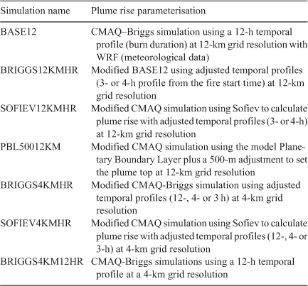
Model plume rise parameterisations
For the Rim Fire, the model was initialised using fire activity data (Sullivan et al. 2008) extracted from the BlueSky Framework using SMARTFIRE2 (Raffuse et al. 2009, 2012). For the Konza Prairie burns, we used field-specific information provided by Konza Prairie’s Biological Station research staff (Table 1). Parametrisation details for each plume rise method are listed in Table 2 (plume rise model parameterisation), Table 3 (algorithm configurations) and Table S3 (model equations). Specific plume rise parameterisations were chosen by their computational cost to implement in an AQM, ease of implementation and availability of parametrisation variables calculated by CMAQ. A major criticism of the standard CMAQ-Briggs PIH calculated on a 12-km grid (hereafter BASE12) is that it is based on experimental data from non-fire plumes (i.e. stack point sources). Another critique is that the buoyancy flux calculation may be inappropriate for large fires (Sofiev et al. 2012; Zhou et al. 2018). To assess these criticisms, we evaluated the CMAQ BASE12 model sensitivity to alternative PIH algorithms, model grid spacing and temporal profiles.
|

|
Model plume rise sensitivities
To evaluate the BASE12 PIH algorithm sensitivity, we tested two models (Table 2, Table S3). The first model was an empirical energy balance parameterisation (like convective cloud formulations) designed for fires (Sofiev et al. 2012), which is implemented at 12- and 4-km grids (hereafter SOFIEV12KMHR and SOFIEV4KMHR). Sofiev is designed to use Fire Radiative Power (FRP); when available, we used the satellite-based measurements, and when not available, it was derived (FRPcalc = heat flux × 0.1 × area burned) using the model heat flux and area burned, assuming that radiative energy was 10% of the total fire heat energy (Wooster et al. 2005; Val Martin et al. 2012). The alternative model was underpinned by a physical rationale based on fire smoke’s general tendency to pool under stable layers (Kahn et al. 2007; Val Martin et al. 2010). This formulation assumes that a smoke plume will reach the PBL and not rise above that layer. The PBL is not a static parameter; therefore, we added 500 m to the PBL maximum value in the model for each hour simulated. This better represented the maximum PIH potential just reaching above the PBL, based on the hourly time-averaged thickness of the model layer used (hereafter PBL50012KM). See section S6 (Sofiev algorithm explanation) and Table S3 (energy balance equations).
Model plume rise comparisons
To evaluate the BASE12 spatial profile sensitivity, a grid spacing of 12 km was compared with the Briggs algorithm at 4 km (hereafter BRIGGS4KMHR); the only difference was the meteorological inputs used at those respective grid resolutions. To evaluate the BASE12 temporal profile sensitivity, as suggested by Zhou et al. (2018), we adjusted the temporal profiles from the national-scale modelling standard 12-h profile (0600–1800 Local Standard Time) to a 3- or 4-h profile (from fire start time) on the 12-km grid (hereafter BRIGGS12KMHR).
Results
Observations
Burn site meteorological conditions and fuels
Table 1 summarises plume rise information for both the 2013 Rim wildfire and 2017 Konza Prairie prescribed fire. Burns 1 and 2 of the Rim Fire (Fig. 1) occurred on 21 and 24 August 2013, respectively, during drought conditions of warm temperatures with low relative humidity (RH < 10%). These conditions caused the fires to spread quickly in winds of 3–10 m s−1 (Peterson et al. 2015). The burned area was greater for Burn 2, but the daily fire spread rate for Burn 1 (503 ha h−1) was double that of Burn 2 (251 ha h−1). At Konza Prairie (Fig. 2), Burns 3 and 4 were conducted on 16 March, and Burn 5 occurred in mid-morning on 20 March (1600 Coordinated Universal Time (UTC)) through early afternoon (2200 UTC). Burns were conducted under the influence of an upper-level trough in a post-frontal air mass and a boundary layer range of 1–2 km by mid-afternoon (2100 UTC). Surface conditions contained a weakening high-pressure system (15 March: 1036.0 hPa; 20 March: 1010.5 hPa), southerly winds (2–5 m s−1) and moderate RH (>20%). The large-scale patterns of wind, temperature and pressure affecting eastern Kansas during each burn were consistent except for temperature and cloud cover. During the burns, the temperature ranged from –4° to 33°C, with low RH of <15%, and light wind speeds of <5.5 m s−1 (Whitehill et al. 2019). The vegetation composition was consistent among burns, with a fuel loading range of 530–630 g m−2 and an average burn rate of 32 ha h−1. Details on the meteorological conditions during the Rim Fire and the Konza Prairie prescribed burns are in Peterson et al. (2015) and Whitehill et al. (2019), respectively. The PBL comparison of the observations with model STL showed that the model performed better for the Konza Prairie prescribed grassland burns (mean bias (MB) of ±400 m)) than for the Rim wildfire (MB of +1000 m; see S3, Planetary boundary layer (PBL) analysis).
Remote sensing of plume heights
Wildfire (Rim Fire)
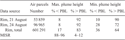
The 2013 California Rim Fire has been described as a massive wildfire, as the data here support. As of 2019, the Rim Fire was California’s fifth largest wildfire. This was also a heavily actioned fire, which was fully contained 9 weeks after the fire ignition. CALIOP plume detrainment data are shown in Figs 3–5 and Table 4. Fig. 3 shows one of several CALIPSO curtains (see Fig. S1 for additional curtains and Fig. S2 for all tracks used), where smoke aerosol data were extracted to develop the daily smoke-plume detainment height products (Fig. 5). Data were extracted from nine CALIPSO curtains to develop the daily smoke evolution for 21 August 2013 (Fig. 5), and seven curtains were extracted for 24 August 2013. Smoke-filled air parcels were injected and detrained into and above the PBL throughout the day on both 21 and 24 August, with plume heights increasing as the afternoon RH decreased and temperatures increased (Fig. 5).
|
The maximum FRP was much higher on 21 August (3025 MW; Fig. 5, Table 4), compared with that on 24 August (max. 1734 MW). The plume was injected over 1 km higher on 21 August from ~1500 local time throughout the day. On all days of the Rim Fire, 83% of the smoke was injected and detrained above the PBL (Table 4); 21 and 24 August were particularly active, with 92% of the smoke detrained above the PBL. The Rim Fire was intense, with much more smoke lofted higher in the atmosphere than is typical. This result contrasts with the larger-scale Multi-angle Imaging SpectroRadiometer (MISR) plume-height analysis (Val Martin et al. 2010), which showed that most smoke (88–96%) remained in the PBL, highlighting the differences in extreme fires compared with ‘normal’ fires. As a result, the standard 12-h assumption was retained.
Prescribed fire (Konza Prairie burns)
The scanning MiniMPL measurements (Fig. 6, Fig. S5) provide evidence that the largest smoke concentrations during the Konza burns were in the advancing portions of the fire. The lidar retrievals showed that smoke from these prairie fires <500 ha tended to pool in the lower PBL (Fig. 7, Table 1), with 17% entering the free troposphere. A comparison of the maximum PIH with the associated maximum backscatter concentrations indicates a contrasting pattern to the standard vertical fire emissions profile, which suggests that some of the smoke reached a higher elevation, but most pooled lower in the PBL. For example, with nearly triple the burn rate, Burn 5 had plumes nearly two to four times higher than Burns 3 and 4 (Fig. 7). For the individual fields <200 ha, smoke generally reached the top of the highest observed layer within the PBL, with some individual plume cores penetrating the PBL. This finding verifies the capping potential of the PBL for prairie fires under these prevailing weather conditions.
The diurnal plume height and intensity from the Konza Prairie burns (Fig. 7) provides additional evidence that small fires (<500 ha) can penetrate the PBL, even if plumes are generated with short burn times (<1–4 h). Plume heights were measured at 600–4100 m, while the PBL range was 750–1270 m. These prescribed fires were consistent with other fires where the meteorological conditions constrained plume rise (e.g. capping inversion), but the burn rate played a lesser role (e.g. Burn 4 plume tops were, on average, 500 m higher than those of Burn 3, with a burn rate difference of only 32 ha h−1). The fuel loading for these fires showed no clear connection to PIH. For example, Burn 4 contained a fuel loading of 942 kg ha−1 (~17%) more than Burn 3, but the resulting plume tops remained relatively similar.
On 20 March 2017, several fields totalling 405 ha burned concurrently in a small area relative to the AQM grid spacing; for this reason, we treated these as one field, Burn 5 (Fig. S5). Burn 5 produced several plumes with distinct cores that were injected 2000–3000 m above the PBL. Plumes that penetrated the PBL continued to rise to higher stable layers (3190 m at 1500–1700 UTC, 3750 m at 1800–2000 UTC). Still, a significant amount of the smoke remained just above the PBL (1300 m), which is consistent with smoke detraining at multiple levels in the atmosphere. Compared with Burn 5, the backscatter intensity of Burns 3 and 4 demonstrated that, as expected, plumes with a lower vertical extent had higher pollution concentrations near the surface.
Model plume rise evaluation
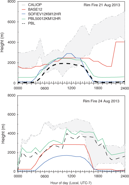
The plume rise evaluation was carried out on an hourly basis, for each model layer, and for each of the five burns we evaluated (Table 1). For the Rim Fire (Burns 1, 2), we used hourly averaged observational data from satellite-based retrievals from CALIOP (Fig. 8: maximum plume tops; Figs S3, S4: mean and minimum heights) to compare with each model formulation. For the Konza Prairie burns (Burns 3, 4, 5), we used hourly averaged ground-based retrievals from the MiniMPL (Figs 9–11).
|

|

|

|
Model with Briggs plume rise evaluation: wildfire (Rim Fire)
For the Rim Fire, the CMAQ-Briggs (BASE12) simulation overall demonstrated the ability to capture the mean PIH range observed (Fig. 8, lower end of the shaded area). The BASE12 simulation successfully captured plume ability from the Rim Fire to penetrate the PBL. The model–observations analysis with BASE12 consisted of an MB of less than ±5–20% compared with the alternative methods. The base simulation compared well with the 3000–5000-m mean plume height value range reported in Peterson et al. (2015). Compared with the observed and other PIH algorithms, BASE12 contained an inherent low bias of 1000 m during the day and a corresponding inherent high bias at night. The night-time plume height appeared to be mostly sporadic and only sometimes within the range of measurements. Similarly, Sofiev et al. (2013) stated that night-time plume height could not be substantiated because of the limited number of observations. These findings suggest that a high bias in particulate matter with a diameter smaller than 2.5 μm (PM2.5), as discussed in Wilkins et al. (2018), could have been skewed by a night-time high bias in PM2.5 and not an overall daily model PM2.5 bias for wildfires.
Model with sensitivities plume rise evaluation: wildfire (Rim Fire)
Comparing the BASE12 run with the SOFIEV12KM12HR method provides additional evidence that BASE12 may underpredict PIH during the daytime for big spread events (12 068 ha day−1) and overpredict PIH for moderate-spread events (6033 ha day−1). The physical rationale method (PBL50012KM) determined that, during the day, PIH showed similar heights to CMAQ-Briggs, when the plume was constrained within the PBL (24 August). For times that the plume was not constrained within the PBL, the accuracy was limited by the height of the PBL. Our simulations did not couple meteorology and fire feedbacks as a system; therefore, we did not expect to capture fire emissions impacts to the PBL locally. This could include, but not be limited to, the impacts from fire heat fluxes directly related to the fire and potential smoke radiative impacts on the PBL (e.g. Kochanski et al. 2019). If the system is not coupled, then this rationale may not be reasonable, because this method relies on plumes not escaping the PBL (e.g. Burn 2).
Model with Briggs plume rise evaluation: prescribed fire (Konza Prairie)
For the prescribed burns (Konza Prairie; Figs 9–11), the BASE12 simulation indicated an overall low PIH bias of 600–2000 m. According to the algorithm differences, the PBL50012KM performed better for the prescribed grassland burns than for the forested wildfire cases (Rim Fire). This difference suggests that the smaller grassland fires (<500 ha) had less impact on the boundary layer physics and contained fewer plumes that escaped the PBL (10–50%). Our results for PBL50012KM are consistent with conclusions from previous studies that when smoke is injected into the free troposphere, it tends to accumulate within atmospheric layers of relative stability aloft (Kahn et al. 2007; Val Martin et al. 2010).
Model with sensitivities plume rise evaluation: prescribed fire (Konza Prairie)
The Sofiev formulation most closely matched these observations. Therefore, we compared the performance of the Sofiev method with the CMAQ-Briggs (BASE12) method. This comparison provided more evidence that the BASE12 model is biased low (Burn 4: BASE12 MB –215.5 m, Sofiev MB –449.2; Burn 5: BASE12 MB –2975.1 m, Sofiev MB –3586.2 m). Lowering the grid spacing from 12 to 4 km provided little improvement in PIH estimates, only slightly increasing the error and bias. This small increase was likely because the meteorological input did not have many differences between the simulations (see S3, Planetary boundary layer (PBL) analysis).
Lastly, using the updated temporal profile, 3–4 h compared with 12 h, the simulation switched the overall PIH estimation bias from negative to positive (e.g. for Burn 3, BASE12 MB –272.4 m; BRIGGS4KM MB 174.8 m). Furthermore, the model’s ability to simulate the overall maximum PIH improved by 200–1000 m. The difference in model performance for estimating PIH for Burns 3 and 4, compared with Burn 5, was because of model design and stability layers. However, CMAQ-Briggs is not designed to capture sharp rising plumes from small fires and rapid changes in the PBL, which typically cap vertical motion.
Model to model plume rise: comparisons and bias
Each model formulation (Table 2) was compared individually with the BASE12 simulation for the maximum PIH, the change in plume top compared with BASE12, and the percentage of plume change above PBL (Fig. 12). All simulations of plume top heights remained below 5000 m for the Rim wildfires and below 2000 m for the prescribed grassland burns at Konza. For the Rim Fire plume heights, a model-to-model comparison showed a 1500–2500-m high bias for both moderate and high-intensity burn days. For the prescribed grassland burns, there was a 50–1000-m low bias across all cases. For the wildfire cases, the base case placed >60% of the plume above the boundary layer, while the other simulation placed 30–55% of the plume above the PBL. For grassland prescribed fires <500 ha, the base case placed <10% of the plume above the PBL, while the alternative model formulations placed 10–50% of the plume above the boundary layer, depending on area burned (e.g. Burn 5) and meteorological situation (e.g. Burn 4). The PBL50012KM simulation placed 50% of the plume above the PBL owing to the way the model was formulated. Therefore, after removing the PBL50012KM simulation, the actual average indicated that, for small fires, 10–35% of the smoke reached above the PBL.

|
Model to observation plume height: comparisons and bias
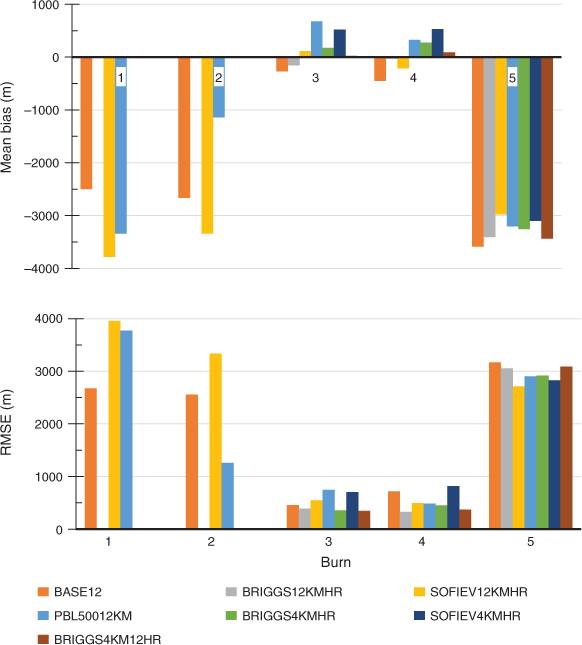
We evaluated the model bias against model formulation changes in plume rise algorithm, grid spacing and temporal allocation (Fig. 13). Overall, the BASE12 model had a consistent low bias of 10–3500 m for the Rim Fire burns. For estimating PIH, the standard base case model performed better (MB –2200 m, RMSE 3000 m) than all alternatives (MB –3500 m, RMSE 3500 m).
|
However, the base case model typically provided PIH estimates with the largest errors and bias for the Konza Prairie prescribed grassland burns. For fires <80 ha, BASE12 with 3–4-h implementation performed best. The model parameterised with Sofiev performed the best for all fires <500 ha, but by a relatively small margin (<400 m). The base model showed the most improvement when changing the temporal allocation (20–1000 m). There was negligible difference between the grid resolution choices (<300 m) owing to the model vertical grid sizes (20 to +500 m, increasing with height). A change lower than 500 m would not be significant computationally unless that model layer was near the PBL. More importantly, an error larger than 500 m could have placed smoke in the incorrect model vertical layer, leading to increased uncertainty in downwind transport (e.g. Burn 5).
Discussion
Improving model performance due to plume rise
The vertical extent of a wildland fire smoke plume is determined by its classification, detection and the fire inventory and modelling system. How a fire is classified or input into a model will determine how, or even if, a plume rise algorithm will be applied to a given fire. Generally, in most AQMs (e.g. CMAQ), only one numerical method is used to simulate plume rise for wildfires and prescribed fires. In some cases, smaller fires will not have adequate plume rise associated with their emissions (Zhou et al. 2018). With a limited sample size of fires, our results suggest that there are benefits to model performance by treating a fire event smoke plume rise with multiple formulations selected based on the event’s size, duration and type (wild or prescribed fire).
Night-time v. daytime plume rise
For large wildland fires, night-time v. daytime plume rise proved to be an area of concern (Sofiev et al. 2013). The night-time high bias in BASE12-estimated plume height might have been due to missing night-time fire characteristics (e.g. model physics, meteorology, intensity, detection). The Burn 2 simulation in the Rim Fire revealed a higher plume height bias during the daytime and a low night-time bias comparable with Sofiev’s method (potentially due to the heat flux value from BlueSky near zero). Furthermore, the heat flux input from the BlueSky framework, although loosely correlated with satellite-derived FRP, tends to underestimate injection height (Kahn et al. 2007; Val Martin et al. 2010, 2012). This may occur if (i) satellite pixels of the order of 1 km2 are only partly filled with a fire (Giglio et al. 2006); (ii) there is overlying smoke opacity (Kahn et al. 2008); or (iii) fire elements have non-unit emissivity, such as smouldering fractions (Val Martin et al. 2018). The suggested solution has been for modellers to multiply heat flux by a factor of 5 or more to match true plume buoyancy (Kahn et al. 2007; Ichoku and Ellison 2014). However, applying this adjustment here did not improve either simulation.
Another concern is that lingering smoke may be captured by observations but missed or ventilated out in model simulations. A full analysis of night-time plume rise for this study was not possible, because no fire observations were taken at night. Another difference between observation and models related to large wildland fires concerned the area burned. For example, plumes from Burns 1 and 2 produced significantly different average observed plume heights (4000–6000-m differences), but model simulations remained similar, in the range of 2000–3000 m. To improve the validation method for modelling, the use of the Soja et al. (2009, 2012) satellite-based method was helpful, because the plume tops derived were within 500–1000 m of those Peterson et al. (2015) and Saide et al. (2015) reported from the same fire.
Temporal allocation – burn duration
For the Konza Prairie small prescribed grassland fires (<500 ha), selecting the proper temporal allocation of emissions and heat fluxes was even more critical than the actual algorithm. For the Rim Fire or larger fires (>5000 to 10 000 ha per day) that do not follow the typical diurnal cycle within an AQMs’ temporal profile, we suggest that it can be better to obtain hourly burned area from, e.g. Geostationary Operational Environmental Satellite (GOES), to estimate fire emissions. Model performance here improved with temporal allocation based on hourly observations but there is potential for greater improvement with the use of a proper treatment of sub-hourly fluctuations. When emissions were allocated based on size of fire and active burning phase, model performance improved significantly (+1000 m). Moreover, there was a connection between model plume heights and stability layers, consistent with earlier studies (e.g. Val Martin et al. 2018). Smoke pooled in stability layers. The stability layer in which a plume would be capped was determined by the strength of that stability layer compared with the energy or lift of an individual plume or buoyancy, a measure of stability calculated as buoyancy frequency. Burn 5 exhibits evidence for the importance of these layers, where plumes that penetrated the PBL continued vertically until reaching the next stable layer at ~3000 m.
Evaluating ways to improve the performance of contemporary AQMs should focus on providing numerically efficient algorithm choices and readily available supplementary data streams. To advance our understanding of smoke dispersion events, the model user should be allowed to select (i) plume rise algorithms based on fire type, and (ii) the time constraints and emission allocation windows. Based on this study, we suggest the following modelling improvements: (i) provide the option to use 4–6 h emissions allocation windows based on the fuel loading and field size, instead of 11 h from the detection time; (ii) if the fire start time is unknown, use the time of fire detection and place the time profile before and after the detection hour (e.g. for a fire detected at 1100 UTC, time profile would be 0900–1300 UTC); (iii) provide for the use of region-specific information such as weather, fuels and burn practices, because these results were highly reflective of the Flint Hills environment and associated fuels (grassland fields) of the Konza Prairie prescribed burn; (iv) allow for variable burn rates, because we found that the optimum estimates for intense to mildly intense fire spread rates were 20–35 ha h−1 for the Flint Hills region, in contrast to 250–500 ha h−1 for the Rim Fire.
Conclusions
Smoke plume injection height (PIH) is an important predictor of how smoke is transported and dispersed downwind of a wildland fire. Most air quality models rely on plume rise methods to determine the vertical allocation of emissions. In this study, we compared several methods with observed PIH. We used the CMAQ modelling system to investigate the impacts of model grid spacing, emissions temporal profile and three plume rise algorithms for five burn events (two wildfire and three prescribed).
Although approaches more advanced than the Briggs algorithm offer the potential to incorporate complex features of wildland fires, our results indicate that the Briggs algorithm performed comparably when provided improved inputs (MB of less than ±5–20% and RMSE lower than 1000 m compared with the alternatives). Our results indicate that the standard model formulation for plume rise has a high bias for large fires (MB range of 1000 to 3000 m). This high bias could be due to a high night-time bias, since the model had a pervasive low daytime bias. Predictions of PIH rely on correctly determining the PBL height. For prescribed grassland burns, the maximum PIH using all approaches was largely underpredicted. However, the bias and mean error, MB of 200 to 600 m and RMSE of 600 to 2000 m, were improved with a more resolved temporal profile (3 to 4 h compared with 12 h). Lastly, the assumption that a rising smoke plume will tend to rest near an STL is valid, but the onus is on the model’s ability to accurately capture those layers. For the large wildfire case (Rim Fire), Briggs placed >60% of the plume above the boundary layer, compared with 83% from observations and 30–55% from alternative models. For the Konza Prairie grassland prescribed fires <500 ha, the Briggs model placed <10% of the plume above the PBL, compared with 17% from observations and 10–35% from alternatives. Thus, the Briggs model performs better if not comparably for wildfires compared with the alternatives while for prescribed fires, Briggs requires adjustments to improve performance.
Based on these findings, we suggest the following modifications to the current air quality modelling system:
Compute plume rise for small fires (<500 ha). Many current models simply inject smoke from small fires into the boundary layer or the lowest model layer.
Assume a temporal profile that more closely matches the active burn period of a prescribed fire. Many models currently assume 12 or 24 h, but this tends to dilute the emissions and heat intensity of these fires.
Assume a fire-specific temporal profile, and if information is not available, apply one of two selectable options:
Take the detection time and generate a temporal profile (e.g. if fire is detected by MODIS or GOES-16/17 at 1100 UTC, time profile applied if using 4 h will be 0900–1300 UTC for the burn).
Use the burn rate or the regional average estimate of area burned (e.g. 35 ha h−1 for the Konza Prairie prescribed burn).
Information on wild and prescribed fire is limited. Therefore, a lack of data persists as an inherent limitation of our study, which only considered the use of a small sample size of fires. But the resulting smoke emissions and impacts are substantial and clear enough to extrapolate relevant findings for future recommendations. Given the findings of this study, we suggest providing a temporal allocation tailored to the types of fires presented. To help with this matter, we urge and suggest that forest agencies, fire land managers and others collect information or create a survey of burn practices by region, season and type of biomass, as indicated in Section 7 of the US EPA National Emissions Inventory documentation (US EPA 2018). Fire plume rise modelling can be improved with the incorporation of space-based retrievals (Soja et al. 2012; Val Martin et al. 2018; Sokolik et al. 2019), databases for plume heights that are not typically modelled (e.g. intense pyrocumulonimbus: Lareau and Clements 2016; Peterson et al. 2017; Wilkins et al. 2020), ground-based measurements (Clements et al. 2018) and fuel consumption rate assessments (van Leeuwen et al. 2014). We recommend that future research explore the potential benefits of a hybrid approach combining multiple algorithms that can be used interchangeably based on conditions encountered by the model. For example, Wilkins et al. (2020) demonstrated a potential for increase in local ozone by 10–80 ppbv downwind of major biomass-burning sources. Plume rise algorithms are not limited to those presented here; in the future, we seek to investigate other methodologies, e.g. the 1-D model of Freitas et al. (2007), in order to evaluate them against observations. Lastly, we suggest an enhanced analysis of the impact of meteorological inputs on plume rise models, which could improve information available to prescribed burn decision-makers (e.g. burn windows, plume dispersion height and direction). These suggested improvements could help enable near-real time model predictions for fire modelling (Marsha and Larkin 2019; Shankar et al. 2019).
Conflicts of interest
The authors declare that they have no conflicts of interest.
Declaration of funding
This research did not receive any specific funding. We are greatly appreciative of NASA funding for the CALIPSO work from the CloudSat and CALIPSO Science Team under grant number NNX16AM30G.
Acknowledgements
The views expressed in this paper are those of the authors and do not necessarily reflect the views or policies of the US EPA. Mention of trade names or commercial products does not constitute an endorsement or recommendation for use. We thank Kansas State University, Nature Conservancy, Konza Prairie Biological Station staff, Micro Pulse LiDAR, part of Hexagon staff, Jacky Rosati-Rowe, Shawn Roselle, Brian Gullet, James Szykman and Russell Long (EPA Office of Research and Development), Andrew Habel (Jacobs Technology, Inc.). Special thanks to Homaira Sharif and Randa Boykin for their graphical assistance. We thank Kirk Baker for assisting with lidar daily operations and Patricia Loesche for editorial comments. Lastly, a special thanks and dedication to the life of Eliza Bradford.
References
Achtemeier GL, Goodrick SA, Liu YQ, Garcia-Menendez F, Hu YT, Odman MT (2011) Modeling smoke plume-rise and dispersion from southern United States prescribed burns with daysmoke. Atmosphere 2, 358–388.| Modeling smoke plume-rise and dispersion from southern United States prescribed burns with daysmoke.Crossref | GoogleScholarGoogle Scholar |
Al-Saadi J, Soja AJ, Pierce RB, Szykman J, Wiedinmyer C, Emmons L, Kondragunta S, Zhang X, Kittaka C, Schaack T, Bowman K (2008) Intercomparison of near-real-time biomass burning emissions estimates constrained by satellite fire data. Journal of Applied Remote Sensing 2, 021504.
| Intercomparison of near-real-time biomass burning emissions estimates constrained by satellite fire data.Crossref | GoogleScholarGoogle Scholar |
Andreae MO, Merlet P (2001) Emission of trace gases and aerosols from biomass burning. Global Biogeochemical Cycles 15, 955–966.
| Emission of trace gases and aerosols from biomass burning.Crossref | GoogleScholarGoogle Scholar |
Baker K, Woody M, Valin L, Szykman J, Yates E, Iraci L, Choi H, Soja A, Koplitz S, Zhou L (2018) Photochemical model evaluation of 2013 California wildfire air quality impacts using surface, aircraft, and satellite data. The Science of the Total Environment 637–638, 1137–1149.
| Photochemical model evaluation of 2013 California wildfire air quality impacts using surface, aircraft, and satellite data.Crossref | GoogleScholarGoogle Scholar | 29801207PubMed |
Baker K, Koplitz S, Foley KM, Hawkins A (2019) Characterizing grassland fire activity in the Flint Hills region and air quality using satellite and routine surface monitor data. The Science of the Total Environment 659, 1555–1566.
| Characterizing grassland fire activity in the Flint Hills region and air quality using satellite and routine surface monitor data.Crossref | GoogleScholarGoogle Scholar | 31096365PubMed |
Baldassarre G, Pozzoli L, Schmidt CC, Unal A, Kindap T, Menzel WP, Whitburn S, Coheur PF, Kavgaci A, Kaiser JW (2015) Using SEVIRI fire observations to drive smoke plumes in the CMAQ air quality model: a case study over Antalya in 2008. Atmospheric Chemistry and Physics 15, 8539–8558.
| Using SEVIRI fire observations to drive smoke plumes in the CMAQ air quality model: a case study over Antalya in 2008.Crossref | GoogleScholarGoogle Scholar |
Briggs GA (1975) Plume rise predictions. In ‘Lectures on air pollution and environmental impact analyses’. (Ed. Haugen, D.) pp. 59–111 (American Meteorological Society: Boston, MA, USA).
Charland AM, Clements CB (2013) Kinematic structure of a wildland fire plume observed by Doppler lidar. Journal of Geophysical Research, D, Atmospheres 118, 3200–3212.
| Kinematic structure of a wildland fire plume observed by Doppler lidar.Crossref | GoogleScholarGoogle Scholar |
Clements CB, Oliphant AJ (2014) The California State University mobile atmospheric profiling system: a facility for research and education in boundary layer meteorology. Bulletin of the American Meteorological Society 95, 1713–1724.
| The California State University mobile atmospheric profiling system: a facility for research and education in boundary layer meteorology.Crossref | GoogleScholarGoogle Scholar |
Clements CB, Potter BE, Zhong S (2006) In situ measurements of water vapor, heat and CO2 fluxes within a prescribed grass fire. International Journal of Wildland Fire 15, 299–306.
| In situ measurements of water vapor, heat and CO2 fluxes within a prescribed grass fire.Crossref | GoogleScholarGoogle Scholar |
Clements CB, Zhong S, Goodrick S, Li J, Bian X, Potter BE, Heilman WE, Charney JJ, Perna R, Jang M, Lee D, Patel M, Street S, Aumann G (2007) Observing the dynamics of wildland grass fires: FireFlux – a field validation experiment. Bulletin of the American Meteorological Society 88, 1369–1382.
| Observing the dynamics of wildland grass fires: FireFlux – a field validation experiment.Crossref | GoogleScholarGoogle Scholar |
Clements CB, Lareau NP, Seto D, Contezac J, Davis B, Teske C, Zajkowski TJ, Hudak AT, Bright BC, Dickinson MB, Butler BW, Jimenez D, Hiers JK (2016) Fire weather conditions and fire–atmosphere interactions observed during low-intensity prescribed fires – RxCADRE 2012. International Journal of Wildland Fire 25, 90–101.
| Fire weather conditions and fire–atmosphere interactions observed during low-intensity prescribed fires – RxCADRE 2012.Crossref | GoogleScholarGoogle Scholar |
Clements CB, Lareau NP, Kingsmill DE, Bowers CL, Camacho CP, Bagley R, Davis B (2018) The Rapid Deployments to Wildfires Experiment (RaDFIRE): observations from the fire zone. Bulletin of the American Meteorological Society 99, 2539–2559.
| The Rapid Deployments to Wildfires Experiment (RaDFIRE): observations from the fire zone.Crossref | GoogleScholarGoogle Scholar |
Colarco PR, Schoeberl MR, Doddridge BG, Marufu LT, Torres O, Welton EJ (2004) Transport of smoke from Canadian forest fires to the surface near Washington, DC: injection height, entrainment, and optical properties. Journal of Geophysical Research 109, D06203.
| Transport of smoke from Canadian forest fires to the surface near Washington, DC: injection height, entrainment, and optical properties.Crossref | GoogleScholarGoogle Scholar |
Fann N, Alman B, Broome RA, Morgan GG, Johnston FH, Pouliot G, Rappold AG (2018) The health impacts and economic value of wildland fire episodes in the US: 2008–2012. The Science of the Total Environment 610–611, 802–809.
| The health impacts and economic value of wildland fire episodes in the US: 2008–2012.Crossref | GoogleScholarGoogle Scholar | 28826118PubMed |
Freitas SR, Longo KM, Andreae MO (2006) Impact of including the plume rise of vegetation fires in numerical simulations of associated atmospheric pollutants. Geophysical Research Letters 33, L17808.
| Impact of including the plume rise of vegetation fires in numerical simulations of associated atmospheric pollutants.Crossref | GoogleScholarGoogle Scholar |
Freitas SR, Longo KM, Chatfield R, Latham D, Silva Dias MAF, Andreae MO, Prins E, Santos JC, Gielow R, Carvalho Jr JA (2007) Including the sub-grid scale plume rise of vegetation fires in low resolution atmospheric transport models. Atmospheric Chemistry and Physics 7, 3385–3398.
| Including the sub-grid scale plume rise of vegetation fires in low resolution atmospheric transport models.Crossref | GoogleScholarGoogle Scholar |
Gelaro R, McCarty W, Suárez MJ, et al. (2017) The Modern-Era Retrospective Analysis for Research and Applications, Version 2 (MERRA-2). Journal of Climate 30, 5419–5454.
| The Modern-Era Retrospective Analysis for Research and Applications, Version 2 (MERRA-2).Crossref | GoogleScholarGoogle Scholar | 32020988PubMed |
Giglio L, Descloitres J, Justice CO, Kaufman YJ (2003) An enhanced contextual fire detection algorithm for MODIS. Remote Sensing of Environment 87, 273–282.
| An enhanced contextual fire detection algorithm for MODIS.Crossref | GoogleScholarGoogle Scholar |
Giglio L, Van der Werf G, Randerson J, Collatz G, Kasibhatla P (2006) Global estimation of burned area using MODIS active fire observations. Atmospheric Chemistry and Physics 6, 957–974.
| Global estimation of burned area using MODIS active fire observations.Crossref | GoogleScholarGoogle Scholar |
Giglio L, Randerson JT, van der Werf GR, Kasibhatla PS, Collatz GJ, Morton DC, DeFries RS (2010) Assessing variability and long-term trends in burned area by merging multiple satellite fire products. Biogeosciences 7, 1171–1186.
| Assessing variability and long-term trends in burned area by merging multiple satellite fire products.Crossref | GoogleScholarGoogle Scholar |
Goodrick SL, Achtemeier GL, Larkin NK, Liu Y, Strand TM (2013) Modelling smoke transport from wildland fires: a review International Journal of Wildland Fire 22, 83–94.
| Modelling smoke transport from wildland fires: a reviewCrossref | GoogleScholarGoogle Scholar |
Gordon M, Makar PA, Staebler RM, Zhang J, Akingunola A, Gong W, Li S-M (2018) A comparison of plume rise algorithms to stack plume measurements in the Athabasca oil sands. Atmospheric Chemistry and Physics 18, 14695–14714.
| A comparison of plume rise algorithms to stack plume measurements in the Athabasca oil sands.Crossref | GoogleScholarGoogle Scholar |
Hyer EJ, Allen DJ, Kasischke ES (2007) Examining injection properties of boreal forest fires using surface and satellite measurements of CO transport. Journal of Geophysical Research 112, D18307.
| Examining injection properties of boreal forest fires using surface and satellite measurements of CO transport.Crossref | GoogleScholarGoogle Scholar |
Ichoku C, Ellison L (2014) Global top–down smoke-aerosol emissions estimation using satellite fire radiative power measurements. Atmospheric Chemistry and Physics 14, 6643–6667.
| Global top–down smoke-aerosol emissions estimation using satellite fire radiative power measurements.Crossref | GoogleScholarGoogle Scholar |
Ichoku C, Kahn R, Chin M (2012) Satellite contributions to the quantitative characterization of biomass burning for climate modelling. Atmospheric Research 111, 1–28.
| Satellite contributions to the quantitative characterization of biomass burning for climate modelling.Crossref | GoogleScholarGoogle Scholar |
Johnston FH, Henderson SB, Chen Y, Randerson JT, Marlier M, Defries RS, Kinney P, Bowman DM, Brauer M (2012) Estimated global mortality attributable to smoke from landscape fires. Environmental Health Perspectives 120, 695–701.
| Estimated global mortality attributable to smoke from landscape fires.Crossref | GoogleScholarGoogle Scholar | 22456494PubMed |
Kahn RA, Li WH, Moroney C, Diner DJ, Martonchik JV, Fishbein E (2007) Aerosol source plume physical characteristics from space-based multi angle imaging. Journal of Geophysical Research, D, Atmospheres 112, D11205.
| Aerosol source plume physical characteristics from space-based multi angle imaging.Crossref | GoogleScholarGoogle Scholar |
Kahn RA, Chen Y, Nelson DL, Leung FY, Li Q, Diner DJ, Logan JA (2008) Wildfire smoke injection heights: Two perspectives from space. Geophysical Research Letters 35, L04809.
| Wildfire smoke injection heights: Two perspectives from space.Crossref | GoogleScholarGoogle Scholar |
Kochanski AK, Mallia DV, Fearon MG, Mandel J, Souri AH, Brown T (2019) Modeling wildfire smoke feedback mechanisms using a coupled fire–atmosphere model with a radiatively active aerosol scheme. Journal of Geophysical Research, D, Atmospheres 124, 9099–9116.
| Modeling wildfire smoke feedback mechanisms using a coupled fire–atmosphere model with a radiatively active aerosol scheme.Crossref | GoogleScholarGoogle Scholar |
Kovalev VS, Newton J, Wold C, Hao WM (2005) Simple algorithm to determine the near-edge smoke boundaries with scanning lidar Applied Optics 44, 1761–1768.
| Simple algorithm to determine the near-edge smoke boundaries with scanning lidarCrossref | GoogleScholarGoogle Scholar |
Labonne M, Bréon F-M, Chevallier F (2007) Injection height of biomass burning aerosols as seen from a spaceborne lidar. Geophysical Research Letters 34, L11806.
| Injection height of biomass burning aerosols as seen from a spaceborne lidar.Crossref | GoogleScholarGoogle Scholar |
Lareau NP, Clements CB (2016) Environmental controls on pyrocumulus and pyrocumulonimbus initiation and development. Atmospheric Chemistry and Physics 16, 4005–4022.
| Environmental controls on pyrocumulus and pyrocumulonimbus initiation and development.Crossref | GoogleScholarGoogle Scholar |
Larkin NK, O’Neill SM, Solomon R, Raffuse S, Strand T, Sullivan DC, Ferguson SA (2009) The BlueSky smoke modeling framework. International Journal of Wildland Fire 18, 906–920.
| The BlueSky smoke modeling framework.Crossref | GoogleScholarGoogle Scholar |
Lelieveld J, Evans JS, Fnais M, Giannadaki D, Pozzer A (2015) The contribution of outdoor air pollution sources to premature mortality on a global scale. Nature 525, 367–371.
| The contribution of outdoor air pollution sources to premature mortality on a global scale.Crossref | GoogleScholarGoogle Scholar | 26381985PubMed |
Leung F-YT, Logan JA, Park R, Hyer E, Kasischke E, Streets D, Yurganov L (2007) Impacts of enhanced biomass burning in the boreal forests in 1998 on tropospheric chemistry and the sensitivity of model results to the injection height of emissions. Journal of Geophysical Research 112, D10313.
| Impacts of enhanced biomass burning in the boreal forests in 1998 on tropospheric chemistry and the sensitivity of model results to the injection height of emissions.Crossref | GoogleScholarGoogle Scholar |
Liu Y-Q, Goodrick S, Achtemeier G, Forbus K, Combs D (2013) Smoke plume height measurement of prescribed burns in the southeastern United States. International Journal of Wildland Fire 22, 130–147.
| Smoke plume height measurement of prescribed burns in the southeastern United States.Crossref | GoogleScholarGoogle Scholar |
Liu Y, Kochanski A, Baker KR, Mell W, Linn R, Paugam R, Mandel J, Fournier A, Jenkins MA, Goodrick S, Achtemeier G, Zhao F, Ottmar R, French NHF, Larkin N, Brown T, Hudak A, Dickinson M, Potter B, Clements C, Urbanski S, Prichard S, Watts A, McNamara D (2019) Fire behaviour and smoke modelling: model improvement and measurement needs for next-generation smoke research and forecasting systems. International Journal Wildland Fire 28, 570–588.
| Fire behaviour and smoke modelling: model improvement and measurement needs for next-generation smoke research and forecasting systems.Crossref | GoogleScholarGoogle Scholar |
Mallia DV, Kochanski AK, Urbanski SP, Lin JC (2018) Optimizing smoke and plume rise modeling approaches at local scales. Atmosphere 9, 166.
| Optimizing smoke and plume rise modeling approaches at local scales.Crossref | GoogleScholarGoogle Scholar |
Marsha A, Larkin NK (2019) A statistical model for predicting PM2.5 for the western United States Journal of the Air & Waste Management Association 69, 1215–1229.
| A statistical model for predicting PM2.5 for the western United StatesCrossref | GoogleScholarGoogle Scholar |
McCarthy N, McGowan H, Guyot A, Dowdy A (2018) MOBILE X-POL RADAR: A new tool for investigating pyroconvection and associated wildfire meteorology. Bulletin of the American Meteorological Society 99, 1177–1195.
| MOBILE X-POL RADAR: A new tool for investigating pyroconvection and associated wildfire meteorology.Crossref | GoogleScholarGoogle Scholar |
McKendry IG, van der Kampa D, Strawbridge KB, Christen A, Crawford B (2009) Simultaneous observations of boundary layer aerosol layers with CL31 ceilometer and 1064/532 nm lidar. Atmospheric Environment 43, 5847–5852.
| Simultaneous observations of boundary layer aerosol layers with CL31 ceilometer and 1064/532 nm lidar.Crossref | GoogleScholarGoogle Scholar |
McKendry IG, Gallagher J, Campuzano P, Bertram A, Strawbridge K, Leaitch R, Macdonald AM (2010) Ground-based remote sensing of an elevated forest fire aerosol layer. Atmospheric Chemistry and Physics 10, 11-921–11-930.
| Ground-based remote sensing of an elevated forest fire aerosol layer.Crossref | GoogleScholarGoogle Scholar |
McKenzie D, Raymond CL, Kellogg L-KB, Norheim RA, Andreu AG, Bayard AC, Kopper KE, Elman E (2007) Mapping fuels at multiple scales: landscape application of the Fuel Characteristic Classification System. Canadian Journal of Forest Research 37, 2421–2437.
| Mapping fuels at multiple scales: landscape application of the Fuel Characteristic Classification System.Crossref | GoogleScholarGoogle Scholar |
Mims SR, Kahn RA, Moroney CM, Gaitley BJ, Nelson DL, Garay MJ (2010) MISR stereo heights of grassland fire smoke plumes in Australia. IEEE Transactions on Geoscience and Remote Sensing 48, 25–35.
| MISR stereo heights of grassland fire smoke plumes in Australia.Crossref | GoogleScholarGoogle Scholar |
Münkel C, Eresmaa N, Räsänen J, Karppinen A (2007) Retrieval of mixing height and dust concentration with lidar ceilometers. Boundary-Layer Meteorology 124, 117–128.
| Retrieval of mixing height and dust concentration with lidar ceilometers.Crossref | GoogleScholarGoogle Scholar |
Omar AH, Winker DM, Vaughan MA, Hu Y, Trepte CR, Ferrare RA, Lee K-P, Hostetler CA, Kittaka C, Rogers RR, Kuehn RE, Liu Z (2009) The Calipso Automated Aerosol Classification and Lidar Ratio selection algorithm. Journal of Atmospheric and Oceanic Technology 26, 1994–2014.
| The Calipso Automated Aerosol Classification and Lidar Ratio selection algorithm.Crossref | GoogleScholarGoogle Scholar |
Ottmar RD, Sandberg DV, Riccardi CL, Prichard SJ (2007) An overview of the fuel characteristic classification system – quantifying, classifying, and creating fuelbeds for resource planning. Canadian Journal of Forest Research 37, 2383–2393.
| An overview of the fuel characteristic classification system – quantifying, classifying, and creating fuelbeds for resource planning.Crossref | GoogleScholarGoogle Scholar |
Paugam R, Wooster M, Freitas S, Val Martin M (2016) A review of approaches to estimate wildfire plume injection height within large-scale atmospheric chemical transport models. Atmospheric Chemistry and Physics 16, 907–925.
| A review of approaches to estimate wildfire plume injection height within large-scale atmospheric chemical transport models.Crossref | GoogleScholarGoogle Scholar |
Peterson DA, Hyer EJ, Campbell JR, Fromm MD, Hair JW, Butler CF, Fenn MA (2015) The 2013 Rim Fire: Implications for predicting extreme fire spread, pyroconvection, and smoke emissions. Bulletin of the American Meteorological Society 96, 229–247.
| The 2013 Rim Fire: Implications for predicting extreme fire spread, pyroconvection, and smoke emissions.Crossref | GoogleScholarGoogle Scholar |
Peterson DA, Hyer EJ, Campbell JR, Solbrig JE, Fromm MD (2017) A conceptual model for development of intense pyrocumulonimbus in western North America. Monthly Weather Review 145, 2235–2255.
| A conceptual model for development of intense pyrocumulonimbus in western North America.Crossref | GoogleScholarGoogle Scholar |
Peterson DA, Campbell J, Hyer E, Fromm M, Kablick G, Cossuth J, DeLand M (2018) Wildfire-driven thunderstorms cause a volcano-like stratospheric injection of smoke. NPJ Climate and Atmospheric Science 1, 30.
| Wildfire-driven thunderstorms cause a volcano-like stratospheric injection of smoke.Crossref | GoogleScholarGoogle Scholar |
Pierce RB, Al‐Saadi JA, Schaack T, et al. (2003) Regional Air Quality Modeling System (RAQMS) predictions of the tropospheric ozone budget over east Asia. Journal of Geophysical Research 108, 8825.
| Regional Air Quality Modeling System (RAQMS) predictions of the tropospheric ozone budget over east Asia.Crossref | GoogleScholarGoogle Scholar |
Pierce RB, Al‐Saadi J, Kittaka C, et al. (2009) Impacts of background ozone production on Houston and Dallas, Texas, air quality during the Second Texas Air Quality Study field mission. Journal of Geophysical Research - Atmospheres 114, D00F09.
| Impacts of background ozone production on Houston and Dallas, Texas, air quality during the Second Texas Air Quality Study field mission.Crossref | GoogleScholarGoogle Scholar |
Pouliot G, Pierce T, Benjey W, O’Neill SM, Ferguson SA (2005) Wildfire emission modeling: integrating BlueSky and SMOKE. In ‘14th Annual International Emission Inventory Conference’, 11–14 April 2005, Las Vegas, NV. (US Environmental Protection Agency: Research Triangle Park, NC) Available at http://www.epa.gov/ttn/chief/conference/ei14/session12/pouliot.pdf [Verified 25 August 2018].
Raffuse S, Wade K, Stone J, Sullivan D, Larkin N, Strand T, Solomon R (2009) Validation of modeled smoke plume injection heights using satellite data. In ‘Eighth Symposium on Fire and Forest Meteorology’, 12–15 October 2009, Kalispell, MT.
Raffuse SM, Craig KJ, Larkin NK, Strand TT, Sullivan DC, Wheeler NJM, Solomon R (2012) An evaluation of modeled plume injection height with satellite-derived observed plume height. Atmosphere 3, 103–123.
| An evaluation of modeled plume injection height with satellite-derived observed plume height.Crossref | GoogleScholarGoogle Scholar |
Rappold AG, Reyes J, Pouliot G, Cascio WE, Diaz-Sanchez D (2017) Community vulnerability to health impacts of wildland fire smoke exposure. Environmental Science & Technology 51, 6674–6682.
| Community vulnerability to health impacts of wildland fire smoke exposure.Crossref | GoogleScholarGoogle Scholar |
Rio C, Hourdin F, Chédin A (2010) Numerical simulation of tropospheric injection of biomass burning products by pyro-thermal plumes. Atmospheric Chemistry and Physics 10, 3463–3478.
| Numerical simulation of tropospheric injection of biomass burning products by pyro-thermal plumes.Crossref | GoogleScholarGoogle Scholar |
Saide PE, Peterson DA, da Silva A, Anderson B, Ziemba LD, Diskin G, Sachse GW, Hair JW, Butler CF, Fenn ME, Jimenez JL, Campuzano-Jost P, Perring AE, Schwarz JP, Markovic MZ, Russell P, Redemann J, Shinozuka Y, Streets DG, Yan F, Dibb JE, Yokelson RJ, Toon OB, Hyer E, Carmichael GR (2015) Revealing important nocturnal and day-to-day variations in fire smoke emissions through a multiplatform inversion. Geophysical Research Letters 42, 3609–3618.
| Revealing important nocturnal and day-to-day variations in fire smoke emissions through a multiplatform inversion.Crossref | GoogleScholarGoogle Scholar |
Shankar U, McKenzie D, Prestemon JP, Baek BH, Omary M, Yang D, Xiu A, Talgo K, Vizuete W (2019) Evaluating wildfire emissions projection methods in comparisons of simulated and observed air quality. Atmospheric Chemistry and Physics 19, 15157–15181.
| Evaluating wildfire emissions projection methods in comparisons of simulated and observed air quality.Crossref | GoogleScholarGoogle Scholar |
Sofiev M, Ermakova T, Vankevich R (2012) Evaluation of the smoke-injection height from wildland fires using remote-sensing data. Atmospheric Chemistry and Physics 12, 1995–2006.
| Evaluation of the smoke-injection height from wildland fires using remote-sensing data.Crossref | GoogleScholarGoogle Scholar |
Sofiev M, Vankevich R, Ermakova T, Hakkarainen J (2013) Global mapping of maximum emission heights and resulting vertical profiles of wildfire emissions. Atmospheric Chemistry and Physics 13, 7039–7052.
| Global mapping of maximum emission heights and resulting vertical profiles of wildfire emissions.Crossref | GoogleScholarGoogle Scholar |
Soja AJ, Al-Saadi JA, Giglio L, Randall D, Kittaka C, Pouliot GA, Kordzi JJ, Raffuse SM, Pace TG, Pierce T, Moore T, Roy B, Pierce B, Szykman JJ (2009) Assessing satellite-based fire data for use in the National Emissions Inventory. Journal of Applied Remote Sensing 3, 031504.
| Assessing satellite-based fire data for use in the National Emissions Inventory.Crossref | GoogleScholarGoogle Scholar |
Soja A, Fairlie T, Westberg D, Pouliot G (2012) Biomass burning plume injection height using CALIOP, MODIS and the NASA Langley Trajectory Model. 2012 US EPA International Emission Inventory Conference. Available at https://www3.epa.gov/ttnchie1/conference/ei20/session7/asoja.pdf [Verified 19 March 2021]
Sokolik IN, Soja AJ, DeMott PJ, Winker D (2019) Progress and challenges in quantifying wildfire smoke emissions, their properties, transport, and atmospheric impacts. Journal of Geophysical Research, D, Atmospheres 124, 13005–13025.
| Progress and challenges in quantifying wildfire smoke emissions, their properties, transport, and atmospheric impacts.Crossref | GoogleScholarGoogle Scholar |
Spinhirne JD (1993) Micro pulse lidar. IEEE Transactions on Geoscience and Remote Sensing 31, 48–55.
| Micro pulse lidar.Crossref | GoogleScholarGoogle Scholar |
Spinhirne JD, Rall JAR, Scott VS (1995) Compact eye-safe lidar systems. The Review of Laser Engineering 23, 112–118.
| Compact eye-safe lidar systems.Crossref | GoogleScholarGoogle Scholar |
Sullivan DC, Raffuse SM, Pryden DA, Craig KJ, Reid SB, Wheeler NJM, Chinkin LR, Larkin NK, Solomon R, Strand T (2008) Development and applications of systems for modeling emissions and smoke from fires: The BlueSky Smoke Modeling Framework and SMARTFIRE. Presented at the 17th International Emissions Inventory Conference led by the Environmental Protection Agency, Portland, OR, USA, 5 June 2008.
Thomas JL, Polashenski CM, Soja AJ, Marelle L, Casey KA, Choi HD, Raut J-C, Wiedinmyer C, Emmons LK, Fast JD, Pelon J, Law KS, Flanner MG, Dibb JE (2017) Quantifying black carbon deposition over the Greenland ice sheet from forest fires in Canada. Geophysical Research Letters 44, 7965–7974.
| Quantifying black carbon deposition over the Greenland ice sheet from forest fires in Canada.Crossref | GoogleScholarGoogle Scholar |
Tosca M, Randerson J, Zender C, Nelson D, Diner D, Logan J (2011) Dynamics of fire plumes and smoke clouds associated with peat and deforestation fires in Indonesia. Journal of Geophysical Research, D, Atmospheres 116, D08207.
| Dynamics of fire plumes and smoke clouds associated with peat and deforestation fires in Indonesia.Crossref | GoogleScholarGoogle Scholar |
Tsaknakis G, Papayannis A, Kokkalis P, Amiridis V, Kambezidis HD, Mamouri RE, Georgoussis G, Avdikos G (2011) Inter-comparison of lidar and ceilometer retrievals for aerosol and Planetary Boundary Layer profiling over Athens, Greece. Atmospheric Measurement Techniques 4, 1261–1273.
| Inter-comparison of lidar and ceilometer retrievals for aerosol and Planetary Boundary Layer profiling over Athens, Greece.Crossref | GoogleScholarGoogle Scholar |
US Environmental Protection Agency (US EPA) (2018) 2014 National Emissions Inventory, Version 2 Technical Support Document. Available at https://www.epa.gov/sites/production/files/2018-07/documents/nei2014v2_tsd_05jul2018.pdf [Verified 19 March 2021]
Val Martin M, Logan JA, Kahn RA, Leung FY, Nelson DL, Diner DJ (2010) Smoke injection heights from fires in North America: Analysis of 5 years of satellite observations. Atmospheric Chemistry and Physics 10, 1491–1510.
| Smoke injection heights from fires in North America: Analysis of 5 years of satellite observations.Crossref | GoogleScholarGoogle Scholar |
Val Martin M, Kahn RA, Logan JA, Paugam R, Wooster M, Ichoku C (2012) Space-based observational constraints for 1-D fire smoke plume-rise models. Journal of Geophysical Research, D, Atmospheres 117, D22204.
| Space-based observational constraints for 1-D fire smoke plume-rise models.Crossref | GoogleScholarGoogle Scholar |
Val Martin M, Kahn RA, Tosca MG (2018) A global analysis of wildfire smoke injection heights derived from space-based multi-angle imaging. Remote Sensing 10, 1609.
| A global analysis of wildfire smoke injection heights derived from space-based multi-angle imaging.Crossref | GoogleScholarGoogle Scholar |
van der Werf GR, Randerson JT, Giglio L, Collatz GJ, Mu M, Kasibhatla PS, Morton DC, DeFries RS, Jin Y, van Leeuwen TT (2010) Global fire emissions and the contribution of deforestation, savanna, forest, agricultural, and peat fires (1997–2009). Atmospheric Chemistry and Physics 10, 11707–11735.
| Global fire emissions and the contribution of deforestation, savanna, forest, agricultural, and peat fires (1997–2009).Crossref | GoogleScholarGoogle Scholar |
van Leeuwen TT, van derWerf GR, Hoffmann AA, Detmers RG, Rücker G, French NHF, Archibald S, Carvalho JA, Cook GD, de Groot WJ, Hély C, Kasischke ES, Kloster S, McCarty JL, Pettinari ML, Savadogo P, Alvarado EC, Boschetti L, Manuri S, Meyer CP, Siegert F, Trollope LA, Trollope WSW (2014) Biomass burning fuel consumption rates: a field measurement database. Biogeosciences 11, 7305–7329.
| Biomass burning fuel consumption rates: a field measurement database.Crossref | GoogleScholarGoogle Scholar |
Walter C, Freitas SR, Kottmeier C, Kraut I, Rieger D, Vogel H, Vogel B (2016) The importance of plume rise on the concentrations and atmospheric impacts of biomass burning aerosol Atmospheric Chemistry and Physics 16, 9201–9219.
| The importance of plume rise on the concentrations and atmospheric impacts of biomass burning aerosolCrossref | GoogleScholarGoogle Scholar |
Welton EJ, Campbell JR (2002) Notes and correspondence: Micropulse lidar signals: uncertainty analysis. Journal of Atmospheric and Oceanic Technology 19, 2089–2094.
| Notes and correspondence: Micropulse lidar signals: uncertainty analysis.Crossref | GoogleScholarGoogle Scholar |
Westphal DL, Toon OB (1991) Simulations of microphysical, radiative, and dynamical processes in continental-scale forest smoke plume. Journal of Geophysical Research 96, 22379–22400.
| Simulations of microphysical, radiative, and dynamical processes in continental-scale forest smoke plume.Crossref | GoogleScholarGoogle Scholar |
Whitehill AR, George I, Long R, Baker KR, Landis M (2019) Volatile organic compound emissions from prescribed burning in Tallgrass Prairie ecosystems. Atmosphere 10, 464.
| Volatile organic compound emissions from prescribed burning in Tallgrass Prairie ecosystems.Crossref | GoogleScholarGoogle Scholar |
Wilkins JL, Pouliot G, Foley K, Appel W, Pierce T (2018) The impact of US wildland fires on ozone and particulate matter: a comparison of measurements and CMAQ model predictions from 2008 to 2012. International Journal of Wildland Fire 27, 684–698.
| The impact of US wildland fires on ozone and particulate matter: a comparison of measurements and CMAQ model predictions from 2008 to 2012.Crossref | GoogleScholarGoogle Scholar |
Wilkins JL, de Foy B, Thompson AM, Peterson DA, Hyer EJ, Graves C, Fishman J, Morris GA (2020) Evaluation of stratospheric intrusions and biomass burning plumes on the vertical distribution of tropospheric ozone over the Midwestern US. Journal of Geophysical Research: Atmospheres 125, e2020JD032454
| Evaluation of stratospheric intrusions and biomass burning plumes on the vertical distribution of tropospheric ozone over the Midwestern US.Crossref | GoogleScholarGoogle Scholar |
Winker D, Vaughan MA, Omar A, Hu Y, Powell KA, Liu Z, Hunt WH, Young SA (2009) Overview of the CALIPSO mission and CALIOP data processing algorithms. Journal of Atmospheric and Oceanic Technology 26, 2310–2323.
| Overview of the CALIPSO mission and CALIOP data processing algorithms.Crossref | GoogleScholarGoogle Scholar |
Wooster MJ, Roberts G, Perry GLW, Kaufman YJ (2005) Retrieval of biomass combustion rates and totals from fire radiative power observations: FRP derivation and calibration relationships between biomass consumption and fire radiative energy release. Journal of Geophysical Research, D, Atmospheres 110, D24311.
| Retrieval of biomass combustion rates and totals from fire radiative power observations: FRP derivation and calibration relationships between biomass consumption and fire radiative energy release.Crossref | GoogleScholarGoogle Scholar |
Wotawa G, Trainer M (2000) The influence of Canadian Forest fires on pollutant concentrations in the United States. Science 288, 324–328.
| The influence of Canadian Forest fires on pollutant concentrations in the United States.Crossref | GoogleScholarGoogle Scholar | 10764643PubMed |
Zhou L, Baker KR, Napelenok SL, Pouliot G, Elleman R, O’Neill SM, Urbanski SP, Wong DC (2018) Modeling crop residue burning experiments to evaluate smoke emissions and plume transport. The Science of the Total Environment 627, 523–533.
| Modeling crop residue burning experiments to evaluate smoke emissions and plume transport.Crossref | GoogleScholarGoogle Scholar | 29426175PubMed |