

Experimental study of the burning characteristics of dead forest fuels
A. Sahila A , H. Boutchiche A , D. X. Viegas B , L. Reis B , C. Pinto B and N. Zekri A *
A Université des Sciences et de la Technologie d’Oran, LEPM BP 1505 El Mnaouer Oran, Algeria.
B Univ Coimbra, ADAI, Department of Mechanical Engineering, Rua Luís Reis Santos, Pólo II, 3030‐788 Coimbra, Portugal.
International Journal of Wildland Fire 32(4) 593-609 https://doi.org/10.1071/WF22088
Submitted: 9 June 2022 Accepted: 4 January 2023 Published: 3 February 2023
© 2023 The Author(s) (or their employer(s)). Published by CSIRO Publishing on behalf of IAWF. This is an open access article distributed under the Creative Commons Attribution-NonCommercial-NoDerivatives 4.0 International License (CC BY-NC-ND)
Abstract
Background: A deeper physical understanding of flame behaviour is necessary to make more reliable predictions about forest fire dynamics.
Aims: To study the container size effect on the combustion characteristics of herbaceous fuels.
Methods: Dead samples were put in cylindrical containers of different sizes, and were ignited at the lowest circumference of the basket in the absence of wind.
Key results: In the growth phase, there is an anomalously fast relaxation of the fuel mass accompanied by a super-diffusion of the emitted gas species, whereas in the decay phase, there is a stretched exponential relaxation and the gas species sub-diffuse through the porous fuel. The crossover between these two anomalous processes occurs when the flame is fully developed. Thomas’s correlation between flame height and fuel bed size, and the two-third power law dependence of the normalised flame height on the Froude number, fit the experimental data well. The flame height variation with burning rate exhibits a hysteresis cycle, implying the existence of memory effects on flame formation.
Conclusions: The observed relaxation regimes and hysteresis cycle seem to drive fire dynamics and behaviour.
Implications: Further investigation of the influence of the fuel geometry and porosity on these properties is necessary.
Keywords: air velocity and temperature profiles, anomalous diffusion, anomalous relaxation, burning rate, flame height, forest fires, hysteresis cycle, turbulent diffusion flame.
Introduction
In the Mediterranean basin, the increasing intensity of forest fires represents a major concern because it seriously disturbs the safeguarding of natural resources, and endangers the ecosystem by affecting the flora and fauna (Pausas et al. 2008; Vilén and Fernandes 2011). Therefore, developing plans that allow firefighters and wildland managers to more effectively control fire spread – and help them to make better decisions on which civilians living in the surroundings depend – is essential. These management plans must be guided by reliable predictions of the fire’s evolution and its thermal impact. To guarantee such rigorous predictions of the complex dynamic behaviour of fire, a deeper understanding and a more accurate estimation of the combustion characteristics (e.g. heat release rate, flame height, temperature, and upward velocity of the induced air) and their correlations are necessary. A large number of experimental works were devoted to examining the behaviour of these parameters in the case of pool fires (Zabetakis and Burgess 1961; Tarifa 1967; Kung and Stavrianidis 1982; Babrauskas 1983; Koseki and Yumoto 1988; Koseki 1989; Klassen and Gore 1994; Chatris et al. 2001), fire whirls (Martin et al. 1976; Lei et al. 2011; Pinto et al. 2017) and natural fires (Thomas 1963; Dupuy et al. 2003; Weise et al. 2005; Sun et al. 2006). Despite all these efforts, more quantitative experimental research is needed to further develop our understanding and optimise the existing numerical and theoretical fire spreading models (see Manzello 2020 and references therein). For instance, some statistical models do not include the physical phenomena governing the combustion process and heat transfer, like percolation (Beer and Enting 1990) and cellular automata (Almeida and Macau 2011). Furthermore, many semi-physical models (like the Small-World Network model; Zekri et al. 2005; Hamamousse et al. 2021) and physical models (Weber 1991; Grishin 1997; Morvan et al. 2009) consider the source’s heat flux either constant during its flaming combustion (residence time) or use a simple Arrhenius law. In addition, even if the heat source term in the Rothermel model is directly related to a reaction velocity (Andrews 2018), it is taken as time-independent. However, the heat released by the burning item was found in earlier works to evolve in three phases: growth; fully developed; and decay (Dupuy et al. 2003; Weise et al. 2005; Sun et al. 2006; Pinto et al. 2017). Among the few works accounting for more realistic heat flux, Vermesi et al. (2016) considered a transient increasing incident flux and proposed a quadratic correlation between the ignition time of the receiving fuel and this flux. Thus, the introduction of a mathematical function that describes accurately the time evolution of the burning rate is crucial for predicting forest fire spread.
This article reports on our experimental study of the burning characteristics of dead straw, representing an herbaceous fuel that can be found in rural or forested areas, in which the turbulent diffusion flame is subjected only to buoyancy forces. Samples of straw were put in cylindrical baskets of different sizes and burned to study the effect of the container diameter on the temporal behaviour of fire. Such cylindrical containers may be representative of single fuel bed items in fire spread modelling. For instance, Adou et al. (2010) considered items of cylindrical shapes to simulate wildfire spread by using the so-called Small-World-Network model. We analysed the time evolution of the burning fuel’s mass within the typical phases of fire development. Novel mathematical tools were used to investigate dynamic relaxation processes that have not previously been reported in fire science literature. Moreover, the temporal evolution of the flame height, temperature, and air-induced velocity were investigated for different container diameters. This allowed for testing of the empirical formulas developed for other fuel types, such as the exponential increase of the mass loss flux with the container diameter (Zabetakis and Burgess 1961; Babrauskas 1983), Thomas correlation for the normalised flame height with the basket size (Thomas 1963), and the power law dependence of the flame height on the Froude number for such a dead forest fuel (Zukoski 1986; Quintiere and Grove 1998; Finney and McAllister 2011; Heskestad 2016).
Experimental setup
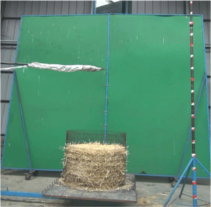
The experiments described in this paper were performed in the Forest Fire Research Laboratory in Lousã, Portugal. They were carried out in a large closed hall with a height of 13 m from the ground to the ceiling, in the absence of air movement inside the laboratory. To study the effect of the container diameter on the burning characteristics of the fuel, straw samples were put in cylindrical containers (baskets) of different sizes, made of a metallic grid, and open on the top (see Fig. 1). These samples had the same initial height (hf = 0.5 m), load ( = Mf/Af = 7.96 kg/m2, Af = π
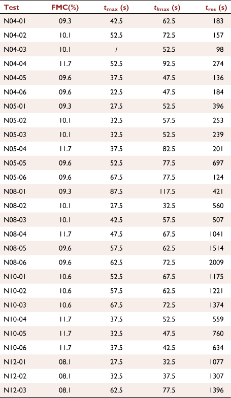
 /4 being the container’s base area), and bulk density (ρf = Mf/Vf = 15.942 kg/m3, with a measured relative uncertainty of 5%, Vf = Af × hf being the volume of the fuel) on a dry basis. The fuel load and bulk density were kept constant by increasing the initial fuel mass Mf and the container diameter dc to keep the initial ratio Mf/Af constant. The volumetric mass density of the particle ρp was 1585 ± 46 kg/m3 (Adapa et al. 2009). Up to six experiments were realised for each basket diameter to ensure the repeatability of tests. Before each experiment, the moisture content of the vegetation was determined by using a moisture analyser A&D MX-50 with a resolution of 0.01%, and the relative humidity of air and ambient temperature were measured by a thermo-hygrometer. The parameters of the tests are given in Table 1, in which each test is referred to by the letter ‘N’, followed by the diameter of the container in dm and a digit indicating the sequence of the test for the given configuration.
|
|
Two K-type thermocouples (nickel–chromium/nickel–aluminium, metallic shielded, with a diameter of 0.5 mm) were used: the first one was put in the centre of the container’s bottom to measure the temperature of the lowest vegetation layer and the second one was 1 m above the fuel surface to determine the flame temperature at this height. An S-Pitot tube was placed at the same distance (1 m) to enable the measurement of the air velocity induced by the flame.
The samples were ignited by a gas burner from the perimeter of the container’s bottom under free-burning conditions. During combustion, the fuel mass decreased over time and its different values were measured using a digital balance (A&D Weighing, HW-100KGL) (10 g resolution) with a frequency of 1 Hz. RSKey v.1.40 software (https://weighing.andonline.com/support/software-downloads/winct) was used to record these values of mass in an Excel file on a laptop. The balance was kept far from the container by using a platform with a lever so that it would not be affected by the heat released by the flame during combustion. Each experiment was recorded by an optical video camera (Sony FDR-AX53) and a digital camera (Canon EOS 550D). The videos were segmented into images by using Free Video to JPG Converter software to measure the flame heights during combustion, and the vertical bar placed near the container allowed a scaling for the flame height obtained in the images to their real values. Although the vertical scale provided by this bar could induce an error of parallax (because it was not in the same plane as the flame’s plane of symmetry), the basket itself could be used in the photos as a vertical scale as well because it was in the flame’s symmetry plane.
Theoretical concepts
In this section, we will briefly discuss the concepts of anomalous relaxation and diffusion that characterise combustion dynamics. Among the numerous non-dimensional equations describing mass fires, those expressing the conservations of mass, momentum, energy, and chemical species in Williams (1969) represent diffusion equations (see the first four equations listed in table 1 of this reference). Diffusion and relaxation are equivalent processes (Metzler and Klafter 2000; Bouchaud 2008). The first process corresponds to a spatiotemporal behaviour of particles in a disturbed system caused by a gradient of concentration, temperature etc., and the second one corresponds to the time evolution of a system from an initial equilibrium state towards a new steady state, after being submitted to an external force.
In the case of small disturbances, the relaxation process is described by a relaxation function ϕ(t) obeying the following differential equation:
The boundary conditions of ϕ are ϕ(t = 0) = 1 and ϕ(t = ∞) = 0 (Stanislavski and Weron 2010). The conservation equations listed in Williams (1969) account only for normal diffusion. In this case, the equivalent relaxation process is described by Eqn 1 with a(t) = 1/τ (constant), and the relaxation function, solution of Eqn 1, is exponentially decreasing with time:

where τ is the relaxation time. In normal diffusion, the particles follow a Brownian motion where the mean square displacement (MSD) is given by <Δx2> = 2dDt (d being the spatial dimension and D the diffusion coefficient). However, in most cases, it is a well-known fact that heterogeneous (complex) systems do not exhibit the above simple exponential relaxation described by Eqn 2. These anomalous relaxation processes are often described by the Kohlrausch–Williams–Watts (KWW) stretched exponential law (Kohlrausch 1854; Williams and Watts 1970):

For β = 1, the normal (exponential) relaxation function Eqn 2 is recovered. If the relaxation process is described by the law Eqn 3 with β > 1, the system exhibits a compressed (squeezed) exponential relaxation. Such non-exponential relaxation phenomena are related to anomalous diffusion processes (Metzler and Klafter 2000; Bouchaud 2008). Indeed, a complex (disordered) medium can severely affect the laws of Brownian motion, which renders the temporal evolution of the Mean Square Deviation of displacement non-linear, <Δx2> ~ tα with α ≠ 1 a real positive number (Metzler and Klafter 2000; Morgado et al. 2002). Here, sub-diffusion (α < 1) and super-diffusion (α > 1) can be distinguished (see Oliveira et al. 2019 for a review). For instance, in the case of wildfires, a sub-diffusion corresponds to an anomalously slow fire propagation induced by the existence of a broad distribution of waiting/ignition times (trapping times) necessary to ignite the nearest neighbour fuels (Sahila et al. 2021). On the other hand, the diffusion of particles in a turbulent flow leads to super-diffusion as demonstrated in the pioneering work of Richardson, interpreted in terms of a non-Fickian process with a scale-dependent diffusion coefficient (Richardson 1926; Bouchaud and Georges 1990; Bourgoin 2015).
Results and discussion
Mass change
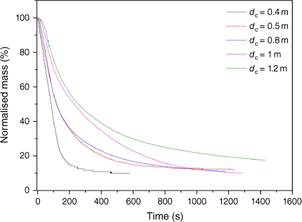
The result of one typical set of experiments for different container sizes are shown in Fig. 2, where the normalised values of the mass Mf/M0 (M0 being the initial mass of the fuel) are plotted as a function of time. As shown in Fig. 2, the fuel’s mass decreases towards an asymptotic minimal value Mfmin for all container sizes. Drysdale (2011) proposed the following equation to describe this tendency:
where K(T) obeys the Arrhenius law K(T) ∝ exp(−EA/RT). EA is the activation energy (J/mol) and R the universal gas constant (8.314 J/K mol). This formula is simplistic because it accounts only for the water evaporation accompanied by volatiles emission during the thermal degradation of the fuel, and does not take into consideration other complex mechanisms involved in this process, such as the scission and formation of molecules and the moisture absorption potential from the surroundings (David 1975). Eqn 4 also describes a relaxation process since the differential Eqn 4 is similar to Eqn 1, where K(T) may depend on time. Instead of Mf, the following relaxation function can be considered:
This function verifies the boundary conditions; ϕ(t = 0) = 1 and ϕ(t = ∞) = 0. It is exponentially decreasing with time (of the form Eqn 2) if K = 1/τ does not depend on temperature (exponential relaxation). If the fuel bed combustion inducing the mass decay yields a varying temperature, an anomalous relaxation is expected to occur. As discussed above, such a process is in general well described by the KWW empirical law given by Eqn 3 (Bouchaud 2008). To verify its existence and determine the exponent β and the relaxation time τ, it is more convenient to use the quantity A(t) instead of ϕ(t):
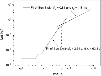
The parameters  and τ are thus deduced from the linear fit of the function A(t) plotted in logarithmic scales, as shown in Fig. 3, which corresponds to a given value of dc. The trend observed in this figure appears for all containers’ diameters. An excellent-fitting correlation coefficient (R2 > 0.99) is observed for all test configurations, with fitting errors smaller than 1%. The curve A(t) shows the existence of a crossover time tx separating two distinct relaxation regimes. For short times t < tx (growth phase), a fitting parameter β > 1 is obtained corresponding to a ‘super-relaxation’. Indeed, in the growth phase, the presence of oxygen and pyrolysis gas allows its rapid spread, accompanied by a super-diffusion of the gas particles through the fuel bed lateral and top surfaces. For sufficiently long times t ≫ tx (decay phase), an exponent β < 1 is obtained corresponding to an anomalously slow relaxation. Indeed, in the decay phase, the whole sample surface is already ignited and the combustion occurs mainly in the bulk, where gas/heat diffusion through the fuel particles is slower (sub-diffusion) compared with that at the surface. This sub-diffusion of the emitted gases corresponds to a mean square displacement exponent α < 1 (see Theoretical concepts section), and may be accompanied by an anomalously slow heat conduction (deviation from Fourier law). Indeed, Li and Wang (2003) demonstrated the existence of a quantitative relation between the thermal conductivity κ and the diffusion exponent α for 1D systems: κ = cLγ (L being the system size) with γ = 2 − 2/α. For α = 1, κ becomes size-independent, and we recover the normal heat conduction process. Around tx, a crossover between an anomalously fast relaxation process (growth phase) and an anomalously slow one (decay phase) occurs. This crossover time is determined from the intersection of the two fitted lines, as shown in Fig. 3.
|
|
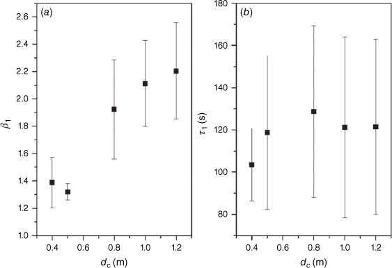
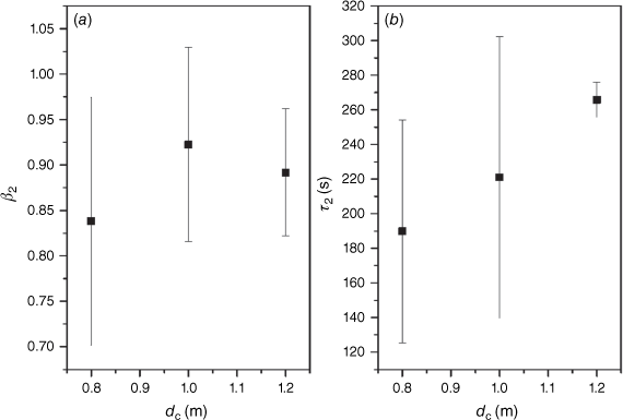
The fitted parameters β and τ in the short- and long-time regimes are plotted in Figs 4 and 5 respectively as a function of the basket diameter. Their values and errors were obtained from six experiments for each diameter. The results show that the exponent β1 is greater than one in the short-time regime (t < tx) for all experiments (see Fig. 4), suggesting that the relaxation process is anomalously fast regardless of the container size. The relaxation time τ1 shows large fluctuations and seems to be independent of the basket diameter. For long times (t ≫ tx), the results in Fig. 5a show that β2 < 1 for all tests, indicating an anomalously slow relaxation regardless of the container’s diameter. For small diameters (dc ≤ 0.5 m, M0 ≤ 1.56 kg), this relaxation process is not observed and is not shown in this figure. The second relaxation time τ2 also presents large fluctuations and seems uncorrelated with dc in Fig. 5b.
|
|
The mass loss rate is a measure of the rate at which the fuel is consumed, and is a key element to understand the combustion dynamics. It is defined as:
The mass loss rate is deduced from the balance data, and its averaged values are estimated at regular intervals (5 s). Note that the heat release rate  = Hf
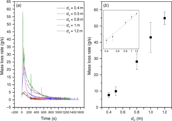
= Hf (in kW) is proportional to the burning rate (the low heat of combustion Hf = 11.7 kJ/g obtained by Pinto et al. (2017) is considered here). The study of the mass loss rate behaviour is then equivalent to that of the heat release rate. The results illustrated in Fig. 6a show the same non-monotonic temporal trend of the mass loss rate regardless of the container diameter. The increase in the burning rate corresponds to the growth phase (super-relaxation observed in Fig. 3), whereas its decrease corresponds to the anomalously slow relaxation occurring in the decay phase. The maximum mass loss rate
  corresponds to the crossover between these two anomalous processes. This maximum mass loss rate increases with dc (see Fig. 6b), as found in the literature for various fuels (Dupuy et al. 2003; Sun et al. 2006) and fire conditions (Martin et al. 1976; Lei et al. 2011; Pinto et al. 2017). It seems to exhibit a power law behaviour with a good fitting exponent around 2 (R² = 0.99), as shown in the inset of Fig. 6b presented in logarithmic scale. This means that each element of the fuel bed surface has the same rate of gas emission in the fully developed phase. When considering an average burning rate value instead of the maximum one
  , a power law correlation is also obtained, but with an exponent smaller than 2. This can be explained by the fact that in the growth and decay phases, only a part of the fuel bed surface is involved in gas emission. The power law exponent can thus be interpreted as an effective dimension D of the fuel bed area involved in gas emission. This effective dimension is around D = 2 when considering the maximum burning rate, and it is close to zero (D → 0) at the beginning or end of the flaming combustion (the flames are localised in small zones of the fuel bed surface). Therefore, it is obvious that averaging the mass loss rate over a given burning duration decreases the effective dimension as this duration increases, with a minimum dimension when considering the entire residence time of the flame. Averaging the burning rate (or equivalently the heat release rate) may mix configurations of merging and less-merging flames (Finney and McAllister 2011), and has a crucial impact on fire spread modelling in the sense that it may lead to false spreading predictions. For instance, an averaging over the residence time of the flame yields a mean heat release rate that can be smaller than the ignition heat flux threshold of the surrounding fuels (Sabi et al. 2021), leading to a non-spreading fire, although the total released energy may be sufficient to ignite these neighbouring items. Because the heat release rate of the burning fuel varies non-linearly with time (Fig. 6a), the only situation where its averaging provides the right spreading predictions occurs when the energy released by the burning item corresponds to the critical energy necessary for igniting the neighbouring items. This energy threshold is given by
  , where qeff is the effective heat flux received by the item and tign is the time to ignition.
|
 vs dc. The inset shows the data on a logarithmic scale.
The time tmax required for the burning rate to reach its maximum value corresponds to the crossover time tx (Fig. 3), and seems to depend only slightly on diameter (within relatively large statistical errors). It ranges between 30 and 90 s for all experiments (Table 1). The duration of the growth phase of the flame may depend on the fuel bed’s initial height, compactness, and bulk density, which are constant for all experiments in this study. Dupuy et al. (2003) proposed an empirical relation to fit the curve  shown in Fig. 6a:
However, this relation is not related to any underlying physical mechanisms such as the dynamic processes discussed above. In the present work, the time-dependent burning rate can be deduced from the expression of the KWW relaxation function Eqns 3 and 5:
with  a constant that depends on the relaxation properties of the fuel and can be interpreted as the mean mass loss rate multiplied by the stretched exponent β. The parameters τ and β appearing in Eqn 9 have the values of (τ1, β1) in the growth phase, and (τ2, β2) in the decay phase. The growth phase of many fires was characterised by a power law increase of the heat release rate
  (kW) with time (
 = α′tp), where p is an exponent that is often found equal to 2, and α′ is the fire growth rate parameter expressed in kW/s2 (Alpert 2016). Note that in Eqn 9, the exponential term becomes nearly constant because the maximum growth duration tmax is always much smaller than the relaxation time τ1 (see Table 1 and Fig. 4b). Thus, the power law growth behaviour observed in different situations (Heskestad 1972; Nelson 1987; Holborn et al. 2004; Alpert 2016) is recovered. The power law exponent (β1 − 1) is constant for large diameters but is much smaller than 2.
The mass loss flux  =
=  /(πD2/4) was widely used for liquid hydrocarbon pool fires, and is proportional to the heat release rate per unit area as discussed above. Zabetakis and Burgess (1961) suggested that, for diameters greater than 0.2 m,
  scales with dc as:

where η and δ are the absorption–extinction coefficient (m−1) and the dimensionless beam length corrector of the flame respectively,  being the mass loss flux for an infinite diameter. Eqn 10 is the spatial analogue of the relaxation function defined by Eqn 2, and the characteristic diameter
  = 1/ηδ is the spatial analogue of the relaxation time. For sufficiently large diameters dc ≫
  , the maximum mass loss flux becomes independent of the container diameter. For liquid pool fires, this equation is valid only for large diameters (dc ≥ 0.2 m) where the combustion is dominated by radiative heat transfer (Babrauskas 1983), the characteristic diameter being
  ≈ 1 m. Babrauskas used the above relation to determine the resulting parameters (
 , η, δ) for some cryogenics, alcohols, simple organic fuels, petroleum products, and solids such as polymethyl-methacrylate, as shown in Table 1 of Babrauskas (1983). It also fits the experimental data for heptane pool fires (Tarifa 1967; Kung and Stavrianidis 1982; Koseki and Yumoto 1988; Koseki 1989; Klassen and Gore 1994; Lei et al. 2011). The most updated review of the burning rate data for pool fires can be found in Viegas et al. (2018). In the present work, contrary to pool fires, the containers have a cylindrical shape with an open lateral surface. Because the vegetation was ignited from the lowest perimeter, volatile gases are emitted during the growth phase from the lateral area of the container and its top surface. Thus, the total area (lateral and top surfaces) should be taken into account for the estimation of
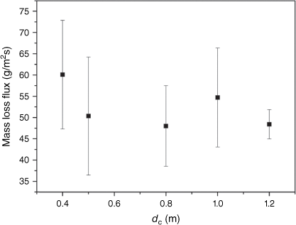
  . However, when the flame is fully developed and the fuel’s burning rate is maximum, the gases are emitted mainly from the top surface. Therefore,
  is defined here as
  /Af. The maximum mass loss flux appears independent of the container diameter within statistical errors, as illustrated in Fig. 7. The saturation regime occurs for diameters greater than 0.4 m (
 < 0.4 m in this study) according to Eqn 10. Moreover, the predominant burning mode that occurs for very large diameters (dc ≥
  ) is radiative and optically thick (Babrauskas 1983).
|
 versus dc.
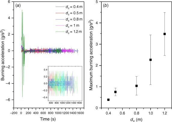
The ‘burning acceleration’ of the fuel  (g/s2) defined as the temporal derivative of the mass loss rate may be a key aspect of fire hazard that is poorly studied. The effect of the container size on
  was already investigated in the case of hydrocarbon pool fires (Chatris et al. 2001), but to the best of our knowledge, it was never studied for forest-type fuels. In Fig. 8a, the temporal evolution curves of
  are illustrated for different diameters of the basket. In the last phase of burning shown in the inset of Fig. 8a, the burning acceleration
  becomes a quasi-periodic function whose amplitudes (around 0.4 g/s) surprisingly seem not affected by the container size. From the analysis of the flame height images, it appears that this quasi-periodic alternation of acceleration and deceleration of the mass loss corresponds either to the last stage of flaming combustion (near the end of the decay phase) or to smouldering combustion. In the first burning phase, large accelerations/decelerations are observed corresponding to the fast-flaming combustion (super-relaxation behaviour observed previously). As expected, the maximum burning acceleration increases with dc (Fig. 8b).
|
 vs dc.
Flame height
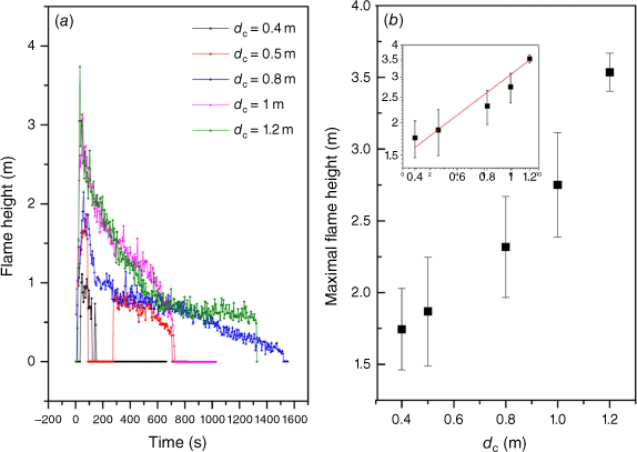
The analysis of the flame heights obtained from the recorded videos (visible images) showed that their temporal behaviour is characterised by the three abovementioned phases: growth, fully developed, and decay. In the first phase, after igniting the perimeter of the lowest layer of the vegetation, the flame spreads vertically very rapidly along the lateral surface, and a consistent flame begins to form accompanied by a horizontal spread of the flames (which merge) through the upper surface of the fuel bed with a continuous increase of the flame height until it attains its peak (after a time tlmax). Then, the fully developed phase with a constant flame height occurs. Afterward, a relatively long period of continuous decrease of the flame height takes place until its extinction (the emitted flammable gases are not sufficient to sustain the flame), where hot glowing embers are formed. The results plotted in Fig. 9a show a typical curve of the flame height’s temporal evolution for a fixed container diameter dc = 1 m for three experiments, where the different phases are illustrated. Photos representing various phases of flame development are presented in Fig. 9b.

|
The time evolution of the flame height l is illustrated in Fig. 10a for different container sizes (one typical set of experiments is presented). In this figure, the flame height trend and its duration (residence time) seem to change clearly as the container’s diameter varies. As illustrated in Figs 6a and 10a, it appears that the maximum mass loss rate of the burning fuel  is always reached earlier than the maximum flame height lmax (Table 1). Sun et al. (2006) suggested a linear dependence of this time shift Δt = tlmax − tmax on the fuel moisture content. Even for a completely dried fuel (FMC = 0%), a temporal delay would still exist because of the time necessary for gas to diffuse through the porous fuel before contributing to the flame. From Table 1, it seems that Δt is slightly affected by the container diameter, because Δt = (23 ± 8) s for dc = 0.4 m, but it is (8 ± 5) s for dc = 1.2 m. A further systematic study of Δt as a function of the fuel bed thickness and moisture content is mandatory to check this dependence.
|
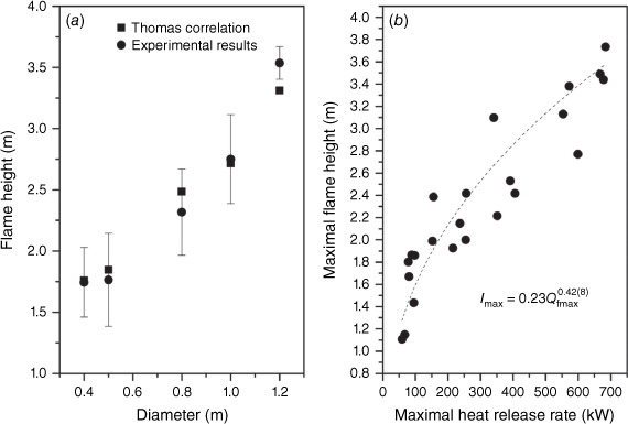
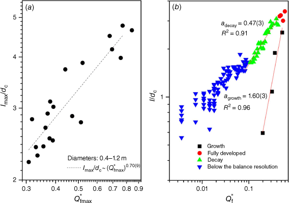
The maximum flame height increases clearly with the container’s size, although with large error bars as illustrated in Fig. 10b. In the inset of this figure (presented in logarithmic scales), lmax fits well a power law dependence on dc (R2 > 0.9), with an exponent of 0.7 ± 0.1. In the case of wood crib fires, Thomas (1963) suggested the following correlation involving the maximum flame height and the container size dc:
where g (m/s2) is the gravity acceleration and ρa (kg/m3) is the air density. This correlation also provides the best fit with experimental data for heptane and hexane pool fires (Bubbico et al. 2016). Recall that from Fig. 7, the maximum mass loss flux  (kg/m2s) is constant within errors. Thus, the power law dependence of lmax on dc observed in the inset of Fig. 10b corresponds to Eqn 11, because the exponent deduced from this equation (0.695) is in agreement with the fitted exponent in the inset of Fig. 10b (0.7 ± 0.1). This agreement is also observed within errors if we compare the maximum flame heights deduced from Thomas correlation (Eqn 11), where the experimental values of
  (Fig. 7) are used, with those obtained from the images (Fig. 11a).
|
 .
.Eqn 11 also shows a power law dependence of lmax on the maximum heat release rate  , which is proportional to
  (see discussion above), the exponent being 0.61. However, although a power law behaviour (lmax =
  ) is well fitted in Fig. 11b (with R2 = 0.9), the exponent (a = 0.42 ± 0.08) seems to correspond unexpectedly to the two-fifth power law exponent instead of 0.61. The two-fifth power law exponent was observed for pool fires (Steward 1970; McCaffrey 1979; Cox and Chitty 1980; Zukoski et al. 1981) and several forest fuels like Pinus pinaster needles and Excelsior (Dupuy et al. 2003), chaparral fuels (Sun et al. 2006) and shrubs (Pinto et al. 2017). The fitting parameters obtained in Fig. 11b are compared with the literature in Table 2. According to eqn 4.33 of Drysdale (2011), a two-fifth exponent corresponds to a flame height independent of the container size, which is not the case here (see Fig. 10b). This apparent discrepancy can be explained by the dependence of both the maximum heat release rate (
 ) and flame height on the container diameter from Figs 6b and 10b (
 ~
~  and lmax ~
  ). Thus, the exponent (0.42 ± 0.08) deduced from the power law fit in Fig. 11b corresponds to 0.35 (lmax ~ (
 )0.7/2) and not to the two-fifth exponent observed in the literature. The mathematical scaling laws governing fire behaviour have been non-dimensionalised, and the relevant dimensionless π-groups have been identified to relate the full scale to model experiments (Williams 1969; Emori and Saito 1983; Quintiere 2020). In fact, Thomas correlation (Eqn 11) relates for crib fires the dimensionless term
  , which expresses the ratio of the fuel flow to gas advection (π10 group in table 1 of Quintiere 2020), to the normalised flame height lmax/dc. Using the expression
  = Hf
= Hf , this term is also the dimensionless heat release rate
  and corresponds to the square root of the Froude number expressing the ratio of the initial momentum to the buoyancy (or π2 group in table 2 of Williams 1969, and π23 of Emori and Saito 1983). Zukoski (1975) introduced a modified dimensionless heat release rate
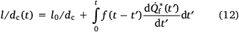
 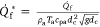 (Ta and cpa being the temperature and specific heat of ambient air). In Fig. 12a, the normalised maximum flame height (lmax/dc) is presented in logarithmic scale as a function of
  (according to the above definition of Zukoski). A power law fit yields an exponent of 0.70 ± 0.09 with a correlation coefficient (R2 ~ 0.8), which is now compatible with the exponent 0.61 appearing in Eqn 11, and may correspond also to the two-third power exponent obtained in the literature. Three regions have been identified to describe the different flame behaviours, ranging from the buoyancy-driven diffusion flames (lmax/dc < 1) where
  < 0.2 (with lmax/dc ~
  2) to jet fires (lmax/dc > 100), where the flame height becomes constant (lmax/dc ~
  0) for a very large Froude number (
 > 100). In this case, the flow is controlled only by momentum (Zukoski 1986; Drysdale 2011). The intermediate region (
 ) corresponds to buoyancy-controlled plume fires, where the normalised flame height is power law increasing with the dimensionless heat release rate
  . Two regimes can be distinguished in the buoyancy plume fires region: one with a power exponent of 2/5, where the flame height is size independent (1 <
  < 10), and the other with a power exponent of 2/3, where the flame height is size dependent (0.2 <
  < 1). The results presented in Fig. 12a correspond to the second regime (0.4 ≤
  ≤ 1), and the fitted two-third power law exponent is consistent with the literature (Thomas 1963; Zukoski 1986; Quintiere and Grove 1998; Drysdale 2011; Finney and McAllister 2011).

|
 ).
).
|
 in logarithmic scale (a) by varying dc at tmax and (b) in the course of time for dc = 1 m.
Now let us examine these correlations over time by fixing dc. Pinto et al. (2017) found a power law correlation between the flame height and burning rate  . Instead of using these parameters, it may be more convenient to use the above-discussed dimensionless parameters (l/dc = f(
 )). The advantage of using these normalised parameters (which do not affect the trend because dc is constant) is that they allow distinguishing the different scaling regimes discussed above. In Fig. 12b, the normalised flame height variation with
  (by varying time) is presented for an arbitrarily chosen diameter. All the phases of flaming combustion (growth, fully developed, and decay) are distinguished in this figure. The time evolution of normalised flame height and heat release rate is not univocal, because the curve l/dc = f(
 ) obtained when the flame height is increasing does not coincide with the one obtained when it is decreasing. The fact that the same input
  can have two positive outputs l/dc suggests the existence of a hysteresis loop. This phenomenon can be expected from the non-monotonic (and asymmetric) evolution with time of the mass loss rate and flame height (Figs 6a, 10a), where the decrease is much slower than the increase. This hysteresis may be attributed to:
a temporal lag between the burning rate and the flame height, corresponding to gas diffusion time and moisture content;
the two different relaxation processes observed in the growth and decay phases;
a memory effect due to the contribution of the rate of gas emission to the flame height since the beginning of the combustion. To the best of our knowledge, this effect has never been investigated in wildland fires. The flame height formation is expected to obey the linear response theory where the effect (l/dc) depends on the entire history of the cause (
 ) as:
) as:
where l0 is the initial flame height and f(t) is the response function of the flame height. For an extensive discussion of linear response theory, see appendix 1.1 of Kremer and Schonhals (2003). Therefore, since the rate of increase of the burning rate (super-relaxation: β > 1) in the growth phase is much larger than the rate of its decrease (sub-relaxation: β < 1) in the decay phase (Figs 3, 4a, 5a), from Eqn 12 the normalised flame height l/dc(t) in the decay phase is larger than that in the growth phase for the same heat release rate  .
.
Fig. 12b is presented on a logarithmic scale, where both growth and decay phases show distinct power law behaviours. Note that both in the growth phase (squares) and decay phase (up triangles), the heat release rate is 0.1 <  < 1, and includes the first and second regions of buoyancy-driven flow (Quintiere and Grove 1998; Finney and McAllister 2011). The linear fit provides the power exponent ai and the intercept bi (the index i denotes the growth and decay phases of flame development):

These parameters may depend on the fuel type, load, wind intensity, etc. The exponent ai is much larger in the growth phase compared with the decay phase in Fig. 12b. For instance, the growth phase (filled squares) characterised by the super-diffusion of gas molecules (see ‘Mass change’ section) yields a power exponent agrowth = 1.60 ± 0.03 (R2 = 0.96). This exponent is smaller than 2 because the flow changes from the first region  ~ 0.1 where l/dc ~
  2 to the intermediate region, with l/dc ~
  2/3 occurring in the fully developed phase of the flame (
 ~ 1). The errors are due to the crossover between these two regions. The decay phase (filled-up triangles) characterised by sub-diffusion of gas yields an exponent adecay = 0.47 ± 0.03 (R2 = 0.91) smaller than the two-third power exponent obtained in the fully developed phase. This may be due to the memory effect, where the flame height remains large because of the contribution of the heat release rate history. The last phase (down triangles) is not considered because it corresponds to burning rates smaller than 10 g/s, which is below the balance resolution, and shows very large flame height fluctuations. The dimensionless heat release rate is much smaller than 0.1, and the flow is most probably in the first region with isolated flames, even though the normalised flame height may be greater than 1.
Because the growth phase is very rapid, there are very few points that render the fit for this phase very inaccurate for some experiments. Therefore, we kept only the values of adecay and bdecay for different container sizes. Data summarised in Table 3 suggest that these exponents are not significantly affected by the basket diameter. The exponents for small diameters (0.4 and 0.5 m) were not presented in this table because all the decay phase occurs for a range of burning rates smaller than 10 g/s (below the balance resolution), which renders the correlation very bad (R2 ≅ 0.6 at best and nearly equal to 0.3 for some experiments).
|
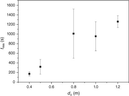
As illustrated in Fig. 13, the residence time of the flame tres increases with dc for small diameters because the available combustible mass M0 increases, whereas it seems to saturate for larger diameters. This saturation may be explained by the subsistence of small localised flames during the last stage of the decay phase, which contributes to making the burning duration longer and renders tres more or less constant within uncertainties. The large fluctuations in the observed residence time (Table 1) depend on the experimental conditions (relative humidity, ambient temperature, etc.). It is worth noting that the residence time tres is not a key parameter in fire spread modelling, as discussed above. Thus, the time within which the heat release rate of the burning vegetation is greater than the critical heat flux for ignition is a more efficient parameter.
|
Temperature and air velocity profiles
Temperature profiles
The time evolution of temperature for both the lower thermocouple (located at the bottom of the basket) and the upper one (located 1 m above the fuel surface) is presented. No corrections to account for heat transfer between the thermocouple and the environment were made to the measured temperature values because it is very difficult to perform such corrections for the thermocouple measurements due to radiation losses during the flame evolution, as explained below (see ‘Upper thermocouple’ section).
Lower thermocouple
The temporal behaviour of the lowest vegetation layer temperature is characterised at least by five stages, as shown in Fig. 14. Because the initial ignition occurs at the perimeter of the basket, the fuel located around the lower thermocouple (at the centre of the basket’s bottom) receives a heat transfer mainly by thermal conduction. Therefore, before the heat reaches the lower thermocouple, this latter remains at ambient temperature during the necessary time for heat diffusion. The container diameter then enhances the duration of this first stage, which fluctuates from one configuration of the fuel particles to another. When the heat reaches the thermocouple, the temperature rises until it reaches the boiling temperature of the water contained in the surrounding fuels. Then a liquid-gas phase transition occurs during a time corresponding to the heat latency (quasi-constant temperature). The heat required to evaporate the mass of water Mw contained in the surrounding particles is given by Q = Mw × Lv, where Lv is the latent heat of vaporisation. From Fig. 14, it seems that the time required for water vaporisation (Mw) increases with dc (larger plateaus). Because the heat of vaporisation Q is expected to be constant with dc (Mw is independent of dc), the heat flux  = Q/t received by these fuel particles decreases by increasing dc. Indeed, the incident heat flux
  induced by the flames at the perimeter is composed of two parts: one contributes to heating the medium (∝mcpdT/dt) and the other one is transferred radially by conduction, radiation and even convection to the nearest neighbour particles. Thus, the heat flux transferred to the container centre (at the thermocouple position) decreases with the diameter. The latency phase observed in Fig. 14 is followed by an ignition phase where the fuel temperature increases abruptly leading to smouldering combustion, the amount of oxygen in the bulk not being sufficient to initiate flaming combustion.
|
Upper thermocouple
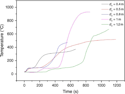
The flame temperature is measured each second by a thermocouple located at 1 m above the fuel surface. Its averaged values, estimated at regular intervals of 5 s, are illustrated in Fig. 15 for different diameters (a typical set of experiments is considered). Before analysing this figure, let’s recall that the flame structure is subdivided into three regions: (1) the lowest region (continuous zone), where the temperature is highest and is constant; (2) the intermittent region (the upper part of the flame), where the temperature decreases inversely with height; and (3) the plume region (above the flame), where smoke temperature decreases as a power law with height (McCaffrey 1979; Babrauskas 2006). The temperature trend shown in Fig. 15a is similar to that of the flame height and burning rate, i.e. it increases in the growth phase towards a maximum temperature, then decreases asymptotically towards ambient temperature. It is worth noting that the thermocouple is located at a fixed vertical distance (1 m) from the fuel surface (see Fig. 1). Therefore, its position relative to the flame tip is varying as the flame height varies. Because of this, the thermocouple measures the temperature at different positions in the flame structure (continuous, intermittent, and plume regions). Indeed, in the first stage of the growth phase (l < 1 m), the thermocouple measures the smoke temperature (plume region), whereas in the fully developed phase (maximum flame height), the thermocouple measures the temperature at the lowest accessible position in the flame (either in the continuous region for large dc or in the intermittent region for small dc), where it is maximum. In particular, for small diameters, the maximal measured temperature does not coincide with the maximum (absolute) flame temperature because the thermocouple is in the intermittent zone (lmax ![]() 1 m, see Fig. 10a). Afterwards, as the flame height is decreasing over time, the thermocouple measures flame temperatures in the intermittent region (l < 1 m), then smoke temperatures in the plume region (l < 1 m).
1 m, see Fig. 10a). Afterwards, as the flame height is decreasing over time, the thermocouple measures flame temperatures in the intermittent region (l < 1 m), then smoke temperatures in the plume region (l < 1 m).
|
As mentioned above, temperature corrections due to radiation losses of the thermocouple cannot be considered because the relative position of the thermocouple in the flame varies with time. In the continuous region, the thermocouple is always surrounded by flames (no radiative losses), whereas in the intermittent zone, it is intermittently inside the flames. Finally, in the plume region, its relative position above the flame tip is increasing. Due to these errors, we assume that the absolute value of the measured temperatures is not accurate; nevertheless, the temporal variation of the temperature indicates a pattern that is consistent with the expected trend (higher temperature values for lower relative positions and vice versa).
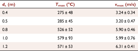
The maximum flame temperatures Tmax for the basket’s diameters considered are summarised in Table 4. The results suggest that Tmax is nearly constant (within statistical errors) for dc ≤ 0.5 m, even if the thermocouple is in the intermittent zone (lmax ![]() 1 m). This is due to the nearly constant position of the thermocouple relative to the flame height (the maximum flame height being nearly constant, as shown in Fig. 10b). For larger diameters where lmax ≫ 1 m, the maximum flame temperature appears constant within errors, although the maximum flame height continues increasing with dc (see Fig. 10b). This confirms the above discussion where the thermocouple position is in the continuous zone according to the definition of McCaffrey (1979).
1 m). This is due to the nearly constant position of the thermocouple relative to the flame height (the maximum flame height being nearly constant, as shown in Fig. 10b). For larger diameters where lmax ≫ 1 m, the maximum flame temperature appears constant within errors, although the maximum flame height continues increasing with dc (see Fig. 10b). This confirms the above discussion where the thermocouple position is in the continuous zone according to the definition of McCaffrey (1979).
|
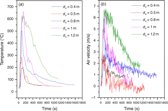
Air velocity profiles
The temporal behaviour of the air velocity induced by the flame measured at 1 m above the fuel’s surface follows the same phases of fire development as illustrated in Fig. 15b. The upward velocity increases when the flame is growing until it attains a maximum magnitude corresponding to the fully developed phase of the flame. Then, a slowing down of the vertical motion of the gas species occurs in the decay phase and remains non-null for some period after the flame extinction. Therefore, the air-flow velocity depends on the vertical position in the flame, which indicates a decrease in the convection heat transfer with the vertical position in the flame. In Table 4, the maximum air velocity dependence on dc shows a different behaviour compared with the initial maximum gas velocity at the boundary between solid and gas phases. Indeed, the initial maximum gas velocity, which is proportional to  according to Eqn 4.2 of Drysdale (2011), is expected to be independent of the basket diameter because the mass loss flux
  is constant, as found in Fig. 7. The gas particles are accelerated in the continuous region where the very high temperatures allow them to overcome gravitation (Cox and Chitty 1980). Thus, the observed high velocity for large diameters (dc ≥ 1 m) is due to the position of the Pitot tube close to the continuous zone, whereas it is near the highest part of the intermittent zone for small diameters (dc ≤ 0.5 m).
Conclusion
Our experimental study of the combustion characteristics of dead straw was realised by burning this fuel in cylindrical baskets of different diameters. The vegetation was ignited from the bottom, and the resulting turbulent diffusion flame was subjected only to buoyancy forces. Time evolution of the burning fuel’s mass loss revealed the existence of an anomalous relaxation process described by the empirical KWW-law. In the growth phase, there was a super-relaxation of the fuel mass accompanied by a super-diffusion of the emitted gas species, whereas in the decay phase, there was an anomalously slow relaxation, and the gas species sub-diffused through the porous fuel. The crossover period between these two anomalous processes corresponds to the fully developed phase where the flame height and the burning rate are maximal. The correlation between the flame height and the fuel container diameter seems to be very well fitted by Thomas’s equation. A power law correlation between the normalised flame height and the Froude number yields a power exponent of 0.70 ± 0.09, which corresponds to the two-third exponent obtained for the buoyancy-driven turbulent flames. The normalised flame height dependence on the heat release rate over time seems to exhibit a hysteresis cycle, implying that the flame height depends on the entire history of the burning rate. This phenomenon can be due to the temporal lag between the flame height and burning rate, and to the two different relaxation processes observed in the growth and decay phases. Further analysis is realised for the behaviour of temperature at the bottom of the fuel bed and over its surface, as well as air velocity at different positions of the flame structure. Further investigations are needed to complete this study. In particular, the relaxation properties of the fuel bed may depend on its geometry and porosity. Moreover, the dynamic behaviours analysed in this paper for dead fuels may be significantly different for live vegetation. Indeed, Darwish et al. (2021) found that the heat transfer from live spruce needles to the adjacent unburned fuel particles is enhanced by micro-explosion-induced ejection of vapours leading to forced convection and increasing the heat release rate. The Froude number may thus be shifted to higher values where the two-fifth power law exponent may occur. On the other hand, the presence of water vapour in the hot volatile jet may slow down the vertical flame spread, leading to a reduced relaxation dynamic. The competition between these two effects may be interesting to investigate.
Nomenclature
Greek symbols
Superscripts
Subscripts
Data availability
The data that support this study are available in the article.
Conflicts of interest
The authors declare no conflicts of interest.
Declaration of funding
The work reported in this article was carried out under the scope of projects McFire (PCIF/MPG/0108/2017), Imfire (PCIF/SSI/0151/2018), SmokeStorm (PCIF/MPG/0147/2019), and SafeFire (PCIF/SSO/0163/2019), and supported by the Portuguese National Science Foundation and European Union’s Horizon 2020 Research and Innovation Programme under grant agreement No. 101003890, FirEUrisk – Developing a Holistic, Risk-Wise Strategy for European Wildfire Management.
Author contributions
Conceptualisation: A. Sahila, N. Zekri and D. X. Viegas; Data curation: A. Sahila, H. Boutchiche, L. Reis and C. Pinto; Formal analysis: A. Sahila, N. Zekri and D.X. Viegas; Methodology: A. Sahila, N. Zekri, H. Boutchiche and D.X. Viegas; Experimental test: A. Sahila, H. Boutchiche, L. Reis and C. Pinto; Supervision: N. Zekri and D.X Viegas; Writing original draft: A. Sahila and N. Zekri; Writing (review & editing): A. Sahila, N. Zekri, D.X. Viegas, H. Boutchiche, L. Reis and C. Pinto.
Acknowledgements
A. Sahila and H. Boutchiche thank the European community for supporting their visit to Coimbra University under the Erasmus framework, where a part of this work was realised. This work was supported by the DGRSDT Algeria (#W1030400).
References
Adapa P, Tabila L, Schoenau G (2009) Compaction characteristics of barley, canola, oat and wheat straw. Biosystemsengineering 104, 335–344.| Compaction characteristics of barley, canola, oat and wheat straw.Crossref | GoogleScholarGoogle Scholar |
Adou JK, Billaud Y, Brou DA, Clerc JP, Consalvi JL, Fuentes A, Kaiss A, Nmira F, Porterie B, Zekri L, Zekri N (2010) Simulating wildfire patterns using a small-world network model. Ecological Modelling 221, 1463–1471.
| Simulating wildfire patterns using a small-world network model.Crossref | GoogleScholarGoogle Scholar |
Almeida RM, Macau EEN (2011) Stochastic cellular automata model for wildland fire spread dynamics. Journal of Physics: Conference Series 285, 012038
| Stochastic cellular automata model for wildland fire spread dynamics.Crossref | GoogleScholarGoogle Scholar |
Alpert RL (2016) Ceiling jet flows. In ‘SFPE Handbook of Fire Protection Engineering’. (Eds MJ Hurley, D Gottuk, JR Hall, K Harada, E Kuligowski, M Puchovsky, J Torero, JM Watts, C Wieczorek) pp. 429–454. (Springer: New York, USA)
Andrews PL (2018) The Rothermel surface fire spread model and associated developments: a comprehensive explanation. General Technical Report RMRSGTR-371. USDA Forest Service, Rocky Mountain Research Station, Fort Collins, CO, USA
Babrauskas V (1983) Estimating large pool fire burning rates. Fire Technology 19, 251–261.
| Estimating large pool fire burning rates.Crossref | GoogleScholarGoogle Scholar |
Babrauskas V (2006) ‘Temperatures in Flames and Fires.’ (Fire Science and Technology: Clarkdale, AZ, USA)
Beer T, Enting IG (1990) Fire spread and percolation modelling. Mathematical and Computer Modelling 13, 77–96.
| Fire spread and percolation modelling.Crossref | GoogleScholarGoogle Scholar |
Bouchaud JP (2008) Anomalous relaxation in complex systems: from stretched to compressed exponentials. In ‘Anomalous Transport: Foundations and Applications’. (Eds HR Klages, G Radons, IM Sokolov) (Wiley-VCH: Berlin, Germany)
| Crossref |
Bouchaud JP, Georges A (1990) Anomalous diffusion in disordered media: statistical mechanisms, models and physical applications. Physics Reports 195, 127–293.
| Anomalous diffusion in disordered media: statistical mechanisms, models and physical applications.Crossref | GoogleScholarGoogle Scholar |
Bourgoin M (2015) Turbulent pair dispersion as a ballistic cascade phenomenology. Journal of Fluid Mechanics 772, 678–704.
| Turbulent pair dispersion as a ballistic cascade phenomenology.Crossref | GoogleScholarGoogle Scholar |
Bubbico R, Dusserre G, Mazzarotta B (2016) Calculation of the flame size from burning liquid pools. Chemical Engineering Transactions 53, 67–72.
| Calculation of the flame size from burning liquid pools.Crossref | GoogleScholarGoogle Scholar |
Chatris JM, Quintela J, Folch J, Planas E, Arnaldos J, Casal J (2001) Experimental study of burning rate in hydrocarbon pool fires. Combustion and Flame 126, 1373–1383.
| Experimental study of burning rate in hydrocarbon pool fires.Crossref | GoogleScholarGoogle Scholar |
Cox G, Chitty R (1980) A study of the deterministic properties of unbounded fire plumes. Combustion and Flame 39, 191–209.
| A study of the deterministic properties of unbounded fire plumes.Crossref | GoogleScholarGoogle Scholar |
Darwish A, Abubaker AM, Salaimeh A, Akafuah NK, Finney M, Forthofer JM, Saito K (2021) Ignition and burning mechanisms of live spruce needles. Fuel 304, 121371
| Ignition and burning mechanisms of live spruce needles.Crossref | GoogleScholarGoogle Scholar |
David C (1975) Thermal degradation of polymers. In ‘Comprehensive Chemical Kinetics’. (Eds CH Bamford, FH Tipper) pp. 1–173. (Elsevier: Amsterdam, Netherlands)
| Crossref |
Drysdale D (Ed.) (2011) ‘An Introduction to Fire Dynamics.’ (A John Wiley & Sons: New York, USA)
Dupuy JL, Maréchal J, Morvan D (2003) Fires from a cylindrical forest fuel burner: combustion dynamics and flame properties. Combustion and Flame 135, 65–76.
| Fires from a cylindrical forest fuel burner: combustion dynamics and flame properties.Crossref | GoogleScholarGoogle Scholar |
Emori RI, Saito K (1983) A study of scaling laws in pool and crib fires. Combustion Science and Technology 31, 217–231.
| A study of scaling laws in pool and crib fires.Crossref | GoogleScholarGoogle Scholar |
Finney MA, McAllister SS (2011) A review of fire interactions and mass fires. Journal of Combustion 2011, 548328
| A review of fire interactions and mass fires.Crossref | GoogleScholarGoogle Scholar |
Grishin AM (1997) ‘Mathematical Modeling of Forest Fires and New Methods of Fighting Them.’ (Publishing House of Tomsk State University: Tomsk, Russia)
Hamamousse N, Kaiss A, Giroud F, Bozabalian N, Clerc J-P, Zekri N (2021) Small World Network Model validation. Case study of Suartone Historical Fire in Corsica. Combustion Science and Technology 194, 3374–3389.
| Small World Network Model validation. Case study of Suartone Historical Fire in Corsica.Crossref | GoogleScholarGoogle Scholar |
Heskestad G (1972) ‘Similarity Relations for the Initial Convective Flow Generated by Fire’. ASME Paper No. 72-WA/HT-17. (American Society of Mechanical Engineers: New York, USA)
Heskestad G (2016) Fire Plumes, Flame Height and Air Entrainment. In ‘SFPE Handbook of Fire Protection Engineering’. (Eds MJ Hurley, D Gottuk, JR Hall, K Harada, E Kuligowski, M Puchovsky, J Torero, JM Watts, C Wieczorek) pp. 396–428. (Springer: New York, USA)
| Crossref |
Holborn PG, Nolan PF, Golt J (2004) An analysis of fire sizes, fire growth rates and times between events using data from fire investigations. Fire Safety Journal 39, 481–524.
| An analysis of fire sizes, fire growth rates and times between events using data from fire investigations.Crossref | GoogleScholarGoogle Scholar |
Klassen ME, Gore JP (1994) Structure and radiation properties of pool fires. Report GCR, 94-651. National Institute of Standards and Technology, Gaithersburg, MD, USA
Kohlrausch R (1854) Theorie des elektrischen Rückstandes in der Leidener Flasche. Annalen der Physik 167, 179–214.
| Theorie des elektrischen Rückstandes in der Leidener Flasche.Crossref | GoogleScholarGoogle Scholar | [In German]
Koseki H (1989) Combustion properties of large liquid pool fires. Fire Technology 25, 241–255.
| Combustion properties of large liquid pool fires.Crossref | GoogleScholarGoogle Scholar |
Koseki H, Yumoto T (1988) Air entrainment and thermal radiation from heptane pool fires. Fire Technology 24, 33–47.
| Air entrainment and thermal radiation from heptane pool fires.Crossref | GoogleScholarGoogle Scholar |
Kremer F, Schonhals A (Eds) (2003) ‘Broadband Dielectric Spectroscopy.’ (Springer-Verlag: Berlin, Germany)
| Crossref |
Kung HC, Stavrianidis P (1982) Buoyant plumes of large-scale pool fires. Symposium (International) on Combustion 19, 905–912.
| Buoyant plumes of large-scale pool fires.Crossref | GoogleScholarGoogle Scholar |
Lei J, Liu N, Zhang L, Chen H, Shu L, Chen P, Deng Z, Zhu J, Satoh K, De Ris JL (2011) Experimental research on combustion dynamics of medium-scale fire whirl. Proceedings of the Combustion Institute 33, 2407–2415.
| Experimental research on combustion dynamics of medium-scale fire whirl.Crossref | GoogleScholarGoogle Scholar |
Li B, Wang J (2003) Anomalous heat conduction and anomalous diffusion in one-dimensional systems. Physical Review Letters 91, 044301
| Anomalous heat conduction and anomalous diffusion in one-dimensional systems.Crossref | GoogleScholarGoogle Scholar |
Manzello SL (2020) ‘Encyclopedia of Wildfires and Wildland–Urban interface (WUI) Fires.’ (Springer Nature: Cham, Switzerland)
| Crossref |
Martin RE, Pendleton DW, Burgess W (1976) Effect of fire whirlwind formation on solid fuel burning rates. Fire Technology 12, 33–40.
| Effect of fire whirlwind formation on solid fuel burning rates.Crossref | GoogleScholarGoogle Scholar |
McCaffrey BJ (1979) Purely buoyant diffusion flames: some experimental results. National Bureau of Standards Interagency/Internal Report (NBSIR) 79-1910, 20234. Center for Fire Research, National Engineering Laboratory, National Bureau of Standards, Washington, DC, USA
Metzler R, Klafter J (2000) The random walk’s guide to anomalous diffusion: a fractional dynamics approach. Physics Reports 339, 1–77.
| The random walk’s guide to anomalous diffusion: a fractional dynamics approach.Crossref | GoogleScholarGoogle Scholar |
Morgado R, Oliveira FA, Batrouni GG, Hansen A (2002) Relation between anomalous and normal diffusion in systems with memory. Physical Review Letters 89, 100601
| Relation between anomalous and normal diffusion in systems with memory.Crossref | GoogleScholarGoogle Scholar |
Morvan D, Méradji S, Accary G (2009) Physical modelling of fire spread in grasslands. Fire Safety Journal 44, 50–61.
| Physical modelling of fire spread in grasslands.Crossref | GoogleScholarGoogle Scholar |
Nelson HE (1987) An engineering analysis of the early stages of fire development – the fire at the Du Pont Plaza hotel and casino – December 31, 1986. National Bureau of Standards Interagency/Internal Report (NBSIR) 87-3560. (US National Institute of Standards and Technology: Gaithersburg, MD, USA)
| Crossref |
Oliveira FA, Ferreira RMS, Lapas LC, Vainstein MH (2019) Anomalous diffusion: a basic mechanism for the evolution of inhomogeneous systems. Frontiers in Physics 7, 18
| Anomalous diffusion: a basic mechanism for the evolution of inhomogeneous systems.Crossref | GoogleScholarGoogle Scholar |
Pausas JG, Llovet J, Rodrigo A, Vallejo R (2008) Are wildfires a disaster in the Mediterranean basin? – A review. International Journal of Wildland Fire 17, 713–723.
| Are wildfires a disaster in the Mediterranean basin? – A review.Crossref | GoogleScholarGoogle Scholar |
Pinto C, Viegas D, Almeida M, Raposo J (2017) Fire whirls in forest fires: an experimental analysis. Fire Safety Journal 87, 37–48.
| Fire whirls in forest fires: an experimental analysis.Crossref | GoogleScholarGoogle Scholar |
Quintiere JG (2020) Scaling realistic fire scenarios. Progress in Scale Modeling, an International Journal 1, 1
| Scaling realistic fire scenarios.Crossref | GoogleScholarGoogle Scholar |
Quintiere JG, Grove BS (1998) A unified analysis for fire plumes. Symposium (International) on Combustion 27, 2757–2766.
| A unified analysis for fire plumes.Crossref | GoogleScholarGoogle Scholar |
Richardson LF (1926) Atmospheric diffusion shown on a distance-neighbour graph. Proceedings of the Royal Society A: Mathematical, Physical and Engineering Sciences 110, 709–737.
| Atmospheric diffusion shown on a distance-neighbour graph.Crossref | GoogleScholarGoogle Scholar |
Sabi FZ, Terrah SM, Mosbah O, Dilem A, Hamamousse N, Sahila A, Harrouz O, Boutchiche H, Chaib F, Zekri N, Kaiss A, Clerc JP, Giroud F, Viegas DX (2021) Ignition/non-ignition phase transition: a new critical heat flux estimation method. Fire Safety Journal 119, 103257
| Ignition/non-ignition phase transition: a new critical heat flux estimation method.Crossref | GoogleScholarGoogle Scholar |
Sahila A, Zekri N, Clerc JP, Kaiss A, Sahraoui S (2021) Fractal analysis of wildfire pattern dynamics using a Small World Network model. Physica A: Statistical Mechanics and its Applications 583, 126300
| Fractal analysis of wildfire pattern dynamics using a Small World Network model.Crossref | GoogleScholarGoogle Scholar |
Stanislavski A, Weron K (2010) Fractional calculus tools applied to study the nonexponential relaxation in dielectrics. In ‘Handbook of Fractional Calculus with Applications. Vol. 4: Applications in Physics, Part A’ (Ed. E Tarasov) pp. 53–70. (De Gruyter: Berlin, Germany)
Steward FR (1970) Prediction of the height of turbulent diffusion buoyant flames. Combustion Science and Technology 2, 203–212.
| Prediction of the height of turbulent diffusion buoyant flames.Crossref | GoogleScholarGoogle Scholar |
Sun L, Zhou X, Mahalingam S, Weise DR (2006) Comparison of burning characteristics of live and dead chaparral fuels. Combustion and Flame 144, 349–359.
| Comparison of burning characteristics of live and dead chaparral fuels.Crossref | GoogleScholarGoogle Scholar |
Tarifa CS (1967) ‘Open Fires; Transport and Combustion of Firebrands.’ (Instituto Nacional de Tecnica Aerospacial Esteban Teradas: Torrejón de Ardoz, Spain)
Thomas PH (1963) The size of flames from natural fires. Symposium (International) on Combustion 9, 844–859.
| The size of flames from natural fires.Crossref | GoogleScholarGoogle Scholar |
Vermesi I, Roenner N, Pironi P, Hadden RM, Rein G (2016) Pyrolysis and ignition of a polymer by transient irradiation. Combustion and Flame 163, 31–41.
| Pyrolysis and ignition of a polymer by transient irradiation.Crossref | GoogleScholarGoogle Scholar |
Viegas DX, Pinto C, Raposo J (2018) Burning Rate. In ‘Encyclopedia of Wildfires and Wildland–Urban Interface (WUI) Fires’. (Ed. S Manzello) (Springer Nature: Cham, Switzerland)
| Crossref |
Vilén T, Fernandes PM (2011) Forest fires in Mediterranean countries: CO2 emissions and mitigation possibilities through prescribed burning. Environmental Management 48, 558–567.
| Forest fires in Mediterranean countries: CO2 emissions and mitigation possibilities through prescribed burning.Crossref | GoogleScholarGoogle Scholar |
Weber RO (1991) Modelling fire spread through fuel beds. Progress in Energy and Combustion Science 17, 67–82.
| Modelling fire spread through fuel beds.Crossref | GoogleScholarGoogle Scholar |
Weise DR, Fletcher T, Smith S, Mahalingam S, Zhou X, Sun L (2005) Correlation of mass loss rate and flame height for live fuels. In ‘Proceedings of the Sixth Symposium, Fire and Forest Meteorology, 27 October 2005, Canmore, AB, Canada’. Available at https://ams.confex.com/ams/6FireJoint/webprogram/Paper97600.html
Williams FA (1969) Scaling mass fires. In ‘Research Abstracts and Reviews. Vol. 11’. (Eds National Academy of Sciences and National Research Council) (The National Academies Press: Washington, DC, USA)
| Crossref |
Williams G, Watts DC (1970) Non-symmetrical dielectric relaxation behaviour arising from a simple empirical decay function. Transactions of the Faraday Society 66, 80–85.
| Non-symmetrical dielectric relaxation behaviour arising from a simple empirical decay function.Crossref | GoogleScholarGoogle Scholar |
Zabetakis MG, Burgess DS (1961) Research on the hazards associated with the production and handling of liquid hydrogen. Report BM-RI-5707. Bureau of Mines, Washington, DC, USA
| Crossref |
Zekri N, Porterie B, Clerc JP, Loraud JC (2005) Propagation in a two-dimensional weighted local small-world network. Physical Review E 71, 046121
| Propagation in a two-dimensional weighted local small-world network.Crossref | GoogleScholarGoogle Scholar |
Zukoski EE (1975) Convective flows associated with room fires. Semi Annual Progress Report. National Science Foundation Grant No. GI 31892 X1. Institute of Technology, Pasadena, CA, USA
Zukoski EE (1986) Fluid dynamic aspects of room fires. Fire Safety Science 1, 1–30.
| Fluid dynamic aspects of room fires.Crossref | GoogleScholarGoogle Scholar |
Zukoski EE, Kubota T, Cetegen B (1981) Entrainment in fire plumes. Fire Safety Journal 3, 107–121.
| Entrainment in fire plumes.Crossref | GoogleScholarGoogle Scholar |