

An escape route planning model based on wildfire prediction information and travel rate of firefighters
Junhao Sheng A , Xingdong Li A * , Xinyu Wang A , Yangwei Wang A , Sanping Li A , Dandan Li A , Shufa Sun B and Lijun Zhao C D
A
B
C
D
Abstract
When firefighters evacuate from wildfires, escape routes are crucial safety measures, providing pre-defined pathways to a safety zone. Their key evaluation criterion is the time it takes for firefighters to travel along the planned escape routes.
While shorter travel times can help firefighters reach safety zones faster, this may expose them to the threat of wildfires. Therefore, the safety of the routes must be considered.
We introduced a new evaluation indicator called the safety index by predicting the growth trend of wildfires. We then proposed a comprehensive evaluation cost function as an escape route planning model, which includes two factors: (1) travel time; and (2) safety of the escape route. The relationship between the two factors is dynamically adjusted through real time factor. The safety window within real time factor provides ideal safety margins between firefighters and wildfires, ensuring the overall safety of escape routes.
Compared with other models, the escape routes planned by the final improved model not only effectively avoid wildfires, but also provide relatively short travel time and reliable safety.
This study ensures sufficient safety margins for firefighters escaping in wildfire environments.
The escape route model described in this study offers a broader perspective on the study of escape route planning.
Keywords: escape route, evacuation, firefighter safety, LANDFIRE, least-cost path modelling, topography, travel rates, wildland fire decision support system.
Introduction
Wildland fires are a serious natural disaster that poses significant threats to both human lives and property (Zhong et al. 2003; Chowdhury and Hassan 2015), and it is crucial to ensure firefighter safety in such dangerous environments. One important safety measure is the establishment of escape routes (National Wildfire Coordinating Group 2016). It serves as pre-defined paths for firefighters to move from their current location to a safety zone during a wildfire (Gleason 1991; Ziegler 2007). The safety zones are locations where the threatened firefighters may find adequate refuge from the danger (Gleason 1991). To ensure the safety and the travel time of escape routes, the escape routes should meet the minimum resistance and risk requirements between the location of the firefighters and the safety zone as much as possible (Dennison et al. 2014; Campbell et al. 2017a). In order to meet the above requirements, it is necessary to study the impact of outdoor landscape conditions and wildfire conditions on firefighters. Therefore, firefighters should have a keen understanding of the surrounding environment. However, the escape process is often hindered by various factors, such as insufficient knowledge of the environment and conditions (Alexander and Thomas 2004), lack of experience (McLennan et al. 2006), and loss of situational awareness (Taynor et al. 1990). Until today, there has been a certain amount of research on the relationship between landscape conditions and the travel rate of firefighters (Davey et al. 1994; Campbell et al. 2017b), as well as established tools and methods for predicting and modelling fire behaviour (e.g. Finney 2004; Finney 2006; Andrews 2014). These provide a good foundation for planning escape routes. However, few studies have comprehensively explored the relationship between two evaluation criteria (escape efficiency and escape safety) and the planning of escape routes.
Previous studies have focused on the influence of slope on travel rate, with some classic models being proposed. For example, Butler et al. (2000) examined the relationship between slope and travel rate using data from two fires with significant firefighter fatalities, while other researchers have developed slope-based travel rate prediction models (e.g. Tobler 1993; Norman 2004). These have found applications in reconstructing historical migration routes (Kantner 2004) and simulating urban natural disaster evacuation (Wood and Schmidtlein 2012). Alexander et al. (2005) conducted experiments on different landscape conditions and firefighter load states, and analysed their impact on travel rates. Recent studies have utilised advanced equipment and rigorous scientific methods to further investigate the relationship between slope and travel rate. For example, Campbell et al. (2019a) employed GPS trajectory databases and LIDAR data to develop percentile models for predicting travel rates based on slope. Sullivan et al. (2020) also proposed three predictive models for slope-travel rate among firefighters in different speeds and states, considering factors such as weight-bearing and age. Campbell et al. (2017b) utilised LIDAR to measure landscape conditions, including slope, vegetation density, and roughness, and quantitatively analysed their relationship with firefighters’ travel rate using a linear mixed effect model.
However, few studies have discussed the impact of the safety of escape routes on their planning. Campbell et al.(2019b) proposed a new concept, Escape Route Index (ERI), which is a new measurement method for evaluating and plotting the escape capability of different areas. Drawing ERI maps before wildfires can help firefighters identify locations with larger exit capacity in advance and reduce the risk of being engulfed by wildfires. Wen et al. (2016) selected terrain undulation and forest density as resistance factors, combined with factors such as fire distribution and wind conditions in wildfires, to construct a wildfire escape path model. But such escape routes cannot be reflected in intuitive travel time. Fryer et al. (2013) developed a theoretical model for predicting spatial evacuation triggers using fire spread and travel rates, but the escape route provided in the model and the escape location for firefighters (starting point) are fixed. There is currently limited research combining the escape route planning of firefighters with wildfire and its growth trajectory. But the prediction technology of wildfire behaviour has provided a good foundation. So far, many models have been proposed to predict the behaviour of wildfires. The existing models are mainly divided into three categories: (1) physical models (e.g. Linn et al. 2002; Mell et al. 2007); (2) empirical models (e.g. Sullivan 2009); (3) and semi-physical and semi-empirical models. Among these, the semi-physical model and semi-empirical model are obtained through ignition experiments based on the physical model and empirical model (e.g. Chen et al. 2022).
To ensure the stability and safety of the escape route in front of wildfires, we also need to consider the impact of wildfire location and its growth trajectory on the escape route. However, there is a lack of understanding of the threat level of the growth trajectory of wildfires to firefighters, which will further affect the safety of escape routes. Therefore, the goal of this study is to establish a suitable comprehensive evaluation cost function as an escape route planning model for real time planning of a safe and fast escape route for firefighters under the threat of wildfire. Therefore, this study proposes: (1) a new evaluation index to explain the threat level of wildfires to different regions, and improve the safety of the route; (2) the real time factor to adaptively adjust the relationship between travel time and safety of escape routes, and ensure both fast and safe evacuation routes in the planning process; and (3) a safety window to ensure the relationship between firefighters and wildfires throughout the entire evacuation process.
Materials and methods
Study area and data download
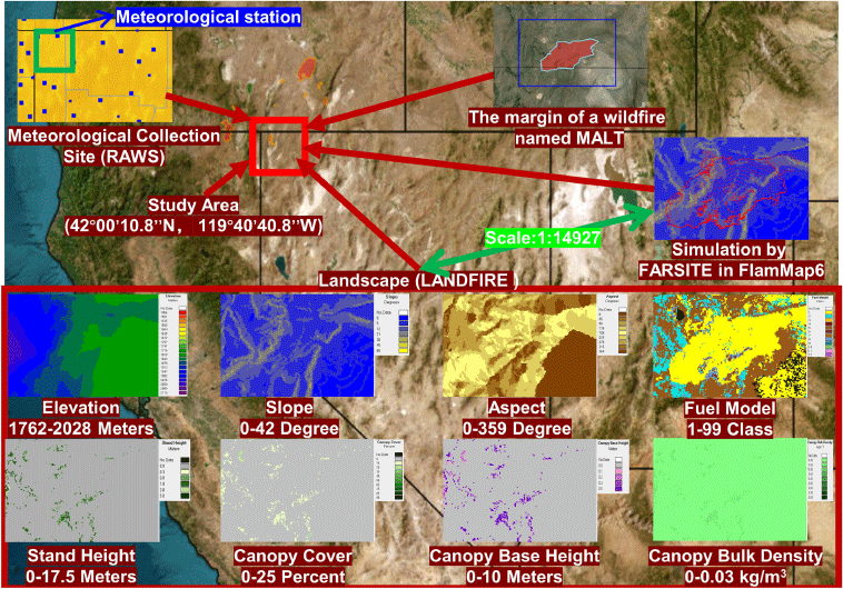
To implement a planning model for escape routes in space, this study selected the Shelton National Antelope Reserve as the research area, located on the border between Nevada and Oregon in the United States (42°00′10.8″N, 119°40′40.8″W) (Fig. 1). The landscape data of the study area are downloaded from LANDFIRE (Rollins 2009), which include elevation, slope, aspect, and fuel model. They have different feature values and their values are reflected by pixels in Fig. 1. The size of the entire landscape file is 159 × 98 grids. The resolution of each grid is 30 m. Considering that the training and testing of the model do not require such a large amount of space, we have locally cropped the above data and conducted subsequent research. There are three reasons for choosing this area: (1) implementing an escape route planning model on an actual spatial scale; (2) the area has rich landscape conditions such as elevation, slope, aspect, and fuel model (Fig. 1); and (3) on 23 July 2014, a fire (named MALT) occurred in the study area, with a burning area of approximately 1087 acres.
Location and information about the study area. The study area has an elevation range of 1762–2028 m, aspect range of 0°–42°, slope range of 0°–359°, fuel model range of 1–99 class, canopy cover range of 0–25%, stand height range of 0–17.5 m, canopy base height range of 0–10 m, and canopy bulk density range of 0–0.03 kg/m3. The scale is 1: 14927.
Generation of predicted wildfire information
The predicted wildfire data were generated using FARSITE in Flammap6 (Finney 2006). The input data for FlamMap6 includes landscape files in the form of GIS grid pixels, meteorological files in the form of data streams and ignition point files. Table 1 shows the information of various input data used to simulate wildfire behaviour. There are meteorological stations in the area. The MALT fire weather were selected as the meteorological data to drive the FARSITE. They were downloaded from the RAWS from 25 August 2010 to 31 August 2010. To obtain more simulation data to test our method, we set up many ignition points in the area before the historical fire occurred, and also simulated the real fire MALT. Finally, the above data were used to predict the future trend of wildfires. Each predicted time frame is 60 min. The areas exceeding 60 min are set to 60.001 min. The reason for setting a 60 min time frame is that the total travel time of the escape routes are within 60 min in this study, so the predicted wildfire information exceeding 60 min is meaningless. Of course, if the escape routes exceed 60 min, the time frame for predicting wildfires can still be extended. However, at this point, it is best to update the actual location of the wildfire and new prediction information midway to ensure the good performance of the model.
| Variable type | Variable name | Unit | Min | Max | Source | |
|---|---|---|---|---|---|---|
| Landscape condition variables | Elevation | Metres | 1762 | 2028 | LANDFIRE | |
| Slope | Degrees | 0 | 42 | |||
| Aspect | Degrees | 0 | 359 | |||
| Fuel model | Class | 1 | 99 | |||
| Canopy cover | Percent | 0 | 25 | |||
| Stand height | Metres | 0 | 17.5 | |||
| Canopy base height | Metres | 0 | 10 | |||
| Canopy bulk density | kg/m3 | 0 | 0.03 | |||
| Climatic factors | Temperature | Fahrenheit | 43 | 83 | RAWS | |
| Relative humidity | Percent | 12 | 77 | |||
| Wind speed | mph | 0 | 23 | |||
| Wind direction | Degrees | 6 | 354 | |||
| Precipitation | mm | 0 | 0 | |||
| Combustible factor variables | Fuel moisture | Percent | 1 | 90 | ||
| Fire point | Coordinates | MTBS | ||||
| Rate correction | Constant | CUSTOMISE |
Traditional method
The original escape route planning method primarily focused on the shortest total travel time (Ttotal, the time for the firefighters to move from their current position to the safety zone) without considering the situation of wildfires. It used predictive travel rate models based on landscape conditions and employed the Dijkstra algorithm (Dijkstra 1959) to generate minimum cost escape routes. This method only used Ttotal as the evaluation criterion, assuming that the shortest total travel time represented the best escape route. The calculation method is as follows:
According to Eqns 1–3 and Fig. 2, n is the current node, which is the current location of the escape personnel; n + 1 is the candidate node around n, which is the escape area that firefighters can choose in the next step; Tman(n, n + 1) is defined as the travel time function, which is the travel time of firefighters from n to the corresponding n + 1; tman(n + 1) is the travel time of firefighters moving forward in the corresponding n + 1; tman(n) is the travel time of firefighters moving forward in n; L is the actual distance of the grid of 30 m; and v is the predicted speed of firefighters in the corresponding area (Eqn 4).
Possible directions for firefighters to move forward at position n. The black arrow lines represent the horizontal or vertical neighbourhood, and the white arrow lines represent the diagonal neighbourhood.

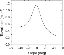
For the purpose of this study, the predicted travel rate model used in this study is based on the slope-travel rate function proposed by Campbell et al. (2019a) (Lorentz 5th percentile) (Fig. 3 and Eqn 4):
where v is predicted velocity in m s−1; θ is slope in degrees; a, b, c, d, and e are constants with the values −1.53, 14.04, 36.81, 0.32, and −0.0027, respectively.
Design of safety index
However, this approach only uses Ttotal as the sole evaluation criterion, and overlooks the location and growth trend of wildfires, which may pose significant risks to firefighters. To address this issue, this study proposes an improvement strategy by introducing a new evaluation function called the Safety index (S). The goal is to form a new comprehensive evaluation function that incorporates both travel time and safety considerations. S represents the difference in the threat of wildfires to two regions. It is calculated based on the predicted time when the wildfire reaches each region. The calculation method of S and the first improved comprehensive evaluation function are:
Eqn 5 is the calculation method for the first improved comprehensive evaluation function model; A and B are the weight coefficients of the travel time function and the safety index function, respectively; Tfire(n) is the predicted time when the wildfire reaches n; and Tfire(n + 1) is the predicted time when the wildfire reaches n + 1;
If S(n, n + 1) is negative, then Tfire(n) < Tfire(n + 1). It indicates that the time for wildfire to spread to region n is shorter than that of region n + 1, indicating region n + 1 is safer. Conversely, when S(n, n + 1) is positive, then Tfire(n) > Tfire(n + 1). It means that the time for wildfire to spread to region n is longer than that of region n + 1, indicating that region n + 1 is more dangerous.
Design of real time factor
Adding S will ensure a certain level of safety in the escape route while also ensuring a shorter Ttotal. However, when planning escape routes, the requirements for safety should not be fixed. Each route selection should be based on the relationship between firefighters and the wildfire. In response to this issue, this study introduces a new parameter, the real time factor (R). Its function is to adjust the proportion of safety index in the entire comprehensive evaluation function. For the design of R, we introduced R1 and R2 for testing (Eqns 7 and 8). It is worth noting that both R1 and R2 can be used as independent R. The functions of R1 and R2 are (Fig. 4):
where R1 is the first real time factor designed; R2 is the second real time factor designed; Tfire is the predicted time when a wildfire arrives at a designated location; Tman is the travel time of firefighters from the starting point to the designated location; X is the Margin of Safety (MOS) (Beighley 1995); and MOS is defined as the difference between the time it takes a fire to reach a given location (Tfire) and the time it takes firefighters to reach that same location (Tman). Ri(n + 1)is the real time factor at the corresponding n + 1 position; Eqn 10 is the calculation method for the comprehensive evaluation function model with added R.
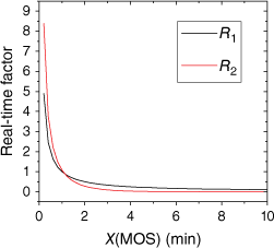
According to Eqns 7, 8 and Fig. 4, the results of R1 and R2 are related to X(MOS). This indicates that the R adjusts the role of the safety index function based on the proximity of the firefighters to the wildfire. And the proximity is MOS in this article. When MOS is small, indicating that firefighters are close to the wildfire, R is assigned a larger value, making the safety index function play a greater role and prioritising areas away from wildfires. Conversely, when the MOS is large, indicating that firefighters are far away from the wildfire, R is assigned a smaller value, making the safety index function play a smaller role and prioritising areas that are easier to travel.
Design of safety window
To provide more flexibility in the relationship between travel time and safety, a safety window (SW) is introduced. The SW acts as a threshold, distinguishing between potential danger times and safety moments. When MOS is less than the SW, it is regarded as a potential danger time, causing R to increase rapidly and allowing S to play a greater role. In contrast, when the MOS is greater than the SW, it is regarded as a safety moment, causing R to decrease rapidly and allowing S to play a smaller role.
The size of SW is manually set and depends on the safety requirements of firefighters for the route. By incorporating the SW, the impact of R is enhanced, allowing for a more nuanced and adaptable approach to escape route planning. The design of R with added SW is shown in Eqns 11 and 12. The R function diagrams for different SW values are (Fig. 5):
where R1-SW and R2-SW are two real time factors optimised by adding SW. Eqn 13 is the calculation method for the comprehensive evaluation function model with added RSW, which will also be used as the final improved model. Ri-SW(n + 1) represents the real-time factor corresponding to region n + 1.
The change of R1 and R2 with different SW value and MOS value. MOS is Margin of Safety. R1–5 indicates that the rea time factor type used is R1, and the value of SW is 5 min.
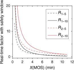
According to Fig. 5, the larger the value of SW, the larger the overall function value of R1-SW and R2-SW. This means that when facing the same situation of MOS, the larger the SW value, the greater the value of Ri-SW. So the role of the safety index is relatively greater.
According to the final model (Eqn 13) and the first improved model (Eqn 5), it can be seen that the two function models combine the travel time function and the safety index function. The travel time function aims for a smaller travel times, allowing firefighters to reach the safety zone faster. The safety index function aims for a smaller value, indicating a safer escape route that ensures the well-being of firefighters. Therefore, the smaller the comprehensive evaluation cost function, the better the result of the escape route.
Results
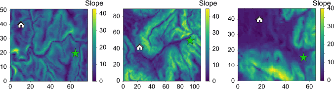
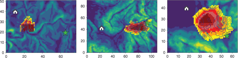
Fig. 6 illustrates the necessary icon information in the image results. Fig. 7 describes the slope parameters of three local areas within the entire study area, and sets and marks the starting point (current location of the escape personnel) and ending point (location of the safety zone) within the three areas. In the simulations, the starting points (the current position of firefighters) are determined randomly near the fire area. The ending points are determined randomly from the area with lower elevation and far from the fire, which is also called the safety zone. The slope range of the three areas is 1–45. Fig. 8 also depicts different wildfire locations and their predicted trends. Each predicted time frame is 60 min. The predicted wildfire spread information for different time periods is distinguished by using different colours. The depiction of escape routes is also divided into the same time periods. The escape route points of different colours represent the routes that firefighters walk during different time periods.
Slope parameters of three study areas (with starting and ending points). The green pentagram represents the starting point (location of the escape personnel), and the white house represents the ending point (location of the safety zone).
Slope parameters of three study areas (with starting point, ending point, current fire location, and predicted results). Maroon represents the part of the current wildfire that is burning; firebrick represents the result of wildfire prediction from 0 to 12 min; indian red represents the result of wildfire prediction for 12–24 min; red represents the results of wildfire prediction for 24–36 min; orange represents the result of wildfire prediction for 36–45 min; and yellow represents the result of wildfire prediction for 48–60 min.
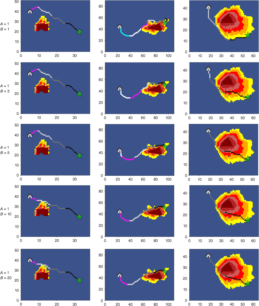
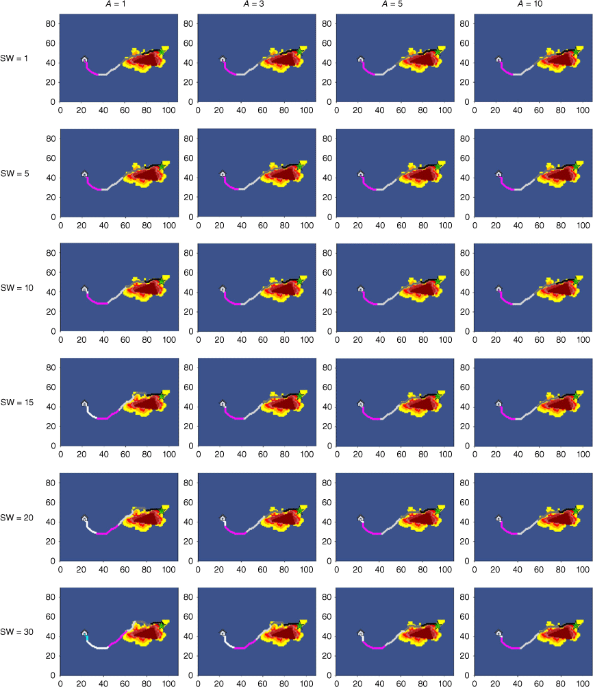
During the training process with the first improved model (Eqn 5), the escape routes generated by testing each group of A and B within the research areas are in Fig. 9. Record Ttotal, Local Minimum MOS (MOSLocal min) and Local Average MOS (MOSLocal avg) under each group of parameter tests are in Fig. 10. (MOSLocal min: The minimum value of MOS for all planned escape route points within the wildfire prediction area. The smaller the MOSLocal min, the worse the escape route, indicating the presence of route points closer to wildfires. MOSLocal avg is the average value of the sum of MOS for all planned escape route points within the wildfire prediction area. The smaller the MOSLocal avg, the closer the overall escape route is to the wildfire, indicating that such an escape route is more unstable.
Partial results of the escape route using the first improved model with different value of A and B.
The results of (a) Total travel time (Ttotal), (b) Local average Margin of Safety (MOSLocal avg) and (c) Local minimum Margin of Safety (MOSLocal min) with changes in A and B in different study areas.
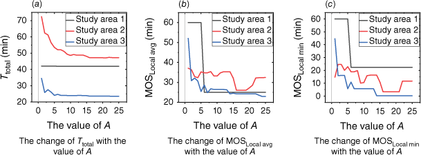
According to Figs 9 and 10, it is evident that the adjustment of the weight coefficient A and B has a significant impact on the planning of escape routes. When A = 1 and B = 1, the escape routes of the three study areas are all planned around the edge of wildfire prediction information, indicating that the safety index plays a greater role at this time and the planning of escape routes prioritise safety over travel time. Therefore, in the subsequent experimental discussion, the default value of B is 1, and only the value of A is adjusted to enhance the effect of the travel time function. When the value of A is relatively small (A = 1.3), although the escape routes are a large Ttotal, they provide sufficiently high MOS. Such high MOS are achieved by sacrificing Ttotal, but it can still meet the needs of firefighters to evacuate from wildfires. A = 1 and A = 3 are used as the parameters for the first improved model. As the value of A increases, all three evaluation indicators decrease. This is because the role of the travel time function in the comprehensive evaluation function is gradually increasing, making the routes more focused on shorter distances. When the value of A is too large (A > 10), Ttotal hardly changes, indicating that the influence of the safety index function is almost ineffective, and the travel time function plays a dominant role. At this point, the MOSLocal min are usually too small, which means firefighters do not have enough MOS to prevent sudden changes in wildfires. The changes in the routes in Fig. 9 are consistent with the above analysis. As the value of A increases, the escape route is shortened by approaching the predicted wildfire area.
In testing the subsequent final model (Eqn 13), the above A and B parameter conditions and study areas need to be used as the basis. First, we excluded obvious adverse situations when A > 10. Second, in the results of study area 1, escape routes are rarely planned in the predicted wildfire information, and the safety index function is calculated based on the predicted wildfire information. This situation limits the effectiveness of the safety index and is not conducive to subsequent discussions. Therefore, only partial A < 10 and study areas 2, 3 were selected as prerequisites. Finally, results of escape routes using the final model are in Figs 11 and 12. Results of three evaluation indicators are in Fig. 13.
Escape route results with different safety windows and weight coefficient A in the same real time factor R2 and study area 2.
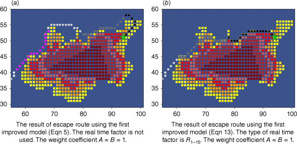
The local comparison graph of the escape routes results between (a) the model with added real time factor and (b) the model without real time factor under the same conditions of study area 2 and the same weight coefficient A = B = 1.
The results of three evaluation indicators of Total travel time (Ttotal), Local average Margin of Safety (MOSLocal avg) and Local minimum Margin of Safety (MOSLocal min) under different conditions (different types of real time factors, different sizes of safety windows, different study areas, and different sizes of parameters A) for (a–c) study area 2 and (d–f) study area 3.
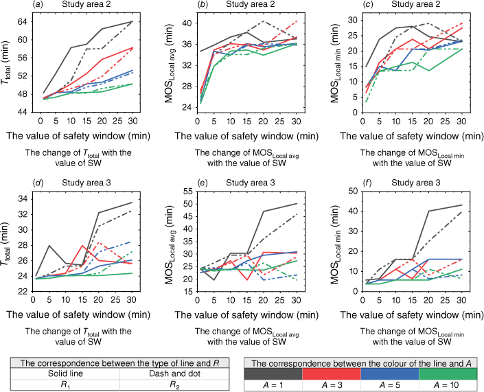
According to Figs 11–13, when comparing escape routes with and without R under the same weight coefficient combination (Fig. 12), the inclusion of R generally leads to better Ttotal. Additionally, smaller values of the SW result in shorter Ttotal and smaller MOSLocal min. This is because the safety index will play a more appropriate role based on the real-time MOS with the addition of R. This helps eliminate unnecessary routes and shorten the Ttotal. The results of MOSLocal avg are generally at high values, indicating that the average safety level of the escape routes is satisfactory. However, there may be some instability in the MOSLocal min, particularly when the value of A is large. When the value of A is small, the MOSLocal min has a good effect, which will correspondingly meet the set SW. However, when SW = 20, 30 min, the MOSLocal min may occasionally fall below the set SW. This instability can be attributed to a large safety window set up and firefighters being relatively close to the fire, making it challenging to meet high safety standards in route selection. As the value of A increases (when A = 3, 5, 10), the MOSLocal min becomes more unstable. While the R has a positive impact on the safety of the escape routes, this impact is also related to the corresponding A and B. When the value of A is large, the travel time function plays a more significant role than the safety index function. As a result, the influence of the R is relatively smaller compared to the travel time function, making it difficult to fully meet the requirements of the SW. Therefore, the larger the value of A, the more likely it is to lead to unstable effects. To ensure that the R has a better impact, it is often not necessary for the A to be too large. This allows for excellent results under various SW settings.
According to Fig. 13 and above analysis, when A = 3, 5, and 10 or when SW = 1 and 5, there are some cases where MOSLocal min is generally small. When SW = 20 and 30, the Ttotal is generally longer. When A = 1 and SW = 10, 15, the escape route not only ensures a relatively short Ttotal, but also provides a relatively reliable MOS. So this article takes A = 1 and SW = 10, 15 as the parameters for the final improved model.
To verify the effectiveness of the escape route algorithm proposed in this article, we compared the traditional method (Eqn 1), the first improved model method (Eqn 5), and the final improved model method (Eqn 13). The main parameter conditions of the methods are known from the above discussion and are in Table 2:
This study conducted simulation experiments under different conditions (including different local research areas, wildfire locations and their predicted information, the starting point of firefighters, and the location of safety zones). Specifically, it reconstructed a new scenario for validation: experimental conditions 1–4 were based on the study area 2 and 3 to continue testing, but the starting and ending points were reset; and experimental conditions 5, 6 are to create a new study area 4, fire information, starting point, and ending point. After testing, Tables 3–5 shows the comparison of Ttotal, MOSLocal avg and MOSLocal min of different methods under different experimental conditions. Fig. 14 shows a comparison of the escape route results for case 5.
| Method 1 | Method 2 | Method 3 | Method 4 | Method 5 | Method 6 | ||
|---|---|---|---|---|---|---|---|
| Case 1 | 53.52 | 57.07 | 54.49 | 54.90 | 54.87 | 54.08 | |
| Case 2 | 17.67 | 30.64 | 19.99 | 19.62 | 20.40 | 18.80 | |
| Case 3 | 46.82 | 72.43 | 61.21 | 59.03 | 57.97 | 50.25 | |
| Case 4 | 23.51 | 34.50 | 27.61 | 25.43 | 25.31 | 25.30 | |
| Case 5 | 34.19 | 43.74 | 39.44 | 39.44 | 36.77 | 34.96 | |
| Case 6 | 34.19 | 41.04 | 39.09 | 40.63 | 38.08 | 35.24 |
| Method 1 | Method 2 | Method 3 | Method 4 | Method 5 | Method 6 | ||
|---|---|---|---|---|---|---|---|
| Case 1 | 14.98 | 46.90 | 24.97 | 34.91 | 26.48 | 31.80 | |
| Case 2 | 21.06 | 52.01 | 31.57 | 30.58 | 31.48 | 26.58 | |
| Case 3 | 25.64 | 37.07 | 32.89 | 38.24 | 38.44 | 36.11 | |
| Case 4 | 22.94 | 52.04 | 32.14 | 30.33 | 29.67 | 29.55 | |
| Case 5 | 22.72 | 44.85 | 34.69 | 34.69 | 33.03 | 31.05 | |
| Case 6 | 26.74 | 0 | 32.77 | 53.09 | 36.00 | 32.39 |
| Method 1 | Method 2 | Method 3 | Method 4 | Method 5 | Method 6 | ||
|---|---|---|---|---|---|---|---|
| Case 1 | 2.10 | 45.52 | 15.44 | 29.76 | 19.66 | 22.78 | |
| Case 2 | 1.08 | 46.81 | 21.81 | 21.81 | 21.81 | 16.70 | |
| Case 3 | 3.51 | 14.70 | 24.63 | 28.09 | 27.88 | 20.73 | |
| Case 4 | 0.30 | 44.63 | 16.07 | 15.94 | 16.12 | 16.13 | |
| Case 5 | 5.30 | 35.68 | 23.21 | 23.21 | 26.07 | 21.61 | |
| Case 6 | 3.02 | 0 | 26.41 | 50.24 | 27.42 | 19.31 |
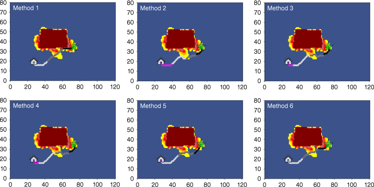
It can be seen that Method 1 has the shortest Ttotal but a very small MOSLocal min. This poses a significant threat to the firefighters, making this escape route unreasonable. However, the other methods may have slightly longer Ttotal, but they provide a better MOSLocal min, ensuring a certain level of safety for the firefighters throughout the entire escape route. Comparing Method 2 with Method 5, it can be seen that Method 5 achieves a shorter Ttotal while still meeting the set SW, thereby improving the overall performance. When compared with Method 3, Method 5 maintains a similar or even shorter Ttotal while obtaining a better MOSLocal min. Similarly, when compared with Method 4, Method 5 generally achieves a shorter Ttotal. Finally, when compared to Method 6, Method 5 may perform slightly worse, but it offers stability under various SW conditions, making it suitable for more demanding scenarios.
Overall, the results indicate that Method 5 provides a balance between travel time and safety, offering a reasonable escape route for different experimental conditions. (note: we simulated a real fire situation named MALT and further validated Method 5 based on this, and still obtained relatively safe and fast escape route results. (see Appendix 1 for details.)
Discussion
One significant finding is the inclusion of the safety index as an additional evaluation indicator for escape route planning in this study. This indicator increases the consideration of the potential threat posed by wildfires to firefighters, rather than just focusing on the total travel time of escape routes. The safety index helps to mitigate the potential harm caused by wildfires along the entire escape route. The results indicate that changes in weight coefficients and R can both affect the role of safety index and subsequently affect the selection of escape routes. Although determining the optimal weight coefficient or R to obtain the optimal escape route is complex, appropriate parameter conditions can produce relatively good results in terms of travel time and safety.
According to Figs 9 and 10, the results of the three groups of escape routes exhibit similar trends, but the changes in parameters A and B have varying degrees of impact on these results. In the first group, it was observed that despite changes in the value of A, the Ttotal remained around 40 min. However, the potential risks to the firefighters varied significantly. This can be attributed to the relatively stable slope of the study area and the distance between firefighters and the wildfire. As a result, there are multiple areas that offer fast passage for the firefighters, leading to similar total travel times but different routes. The inclusion of a safety index allows for better avoidance of wildfire areas and facilitates reaching safe areas. The results of the second and third groups are noticeably influenced by changes in the A and B. This can be attributed to the starting point of the escape personnel being closer to the wildfire, which inevitably impacts the selection of escape routes based on the safety index. Although the trends in the results are similar, there are specific differences. In the second group, Ttotal gradually stabilises when the value of A is 10. While in the third group, Ttotal stabilises when the value of A is 5. According to Fig. 8, these differences are partly due to the fact that in the same 60 min prediction time, the third group of wildfires propagated faster and more widely, resulting in the calculated safety index function of the third group being usually smaller than that of the second group. Consequently, the impact of the safety index in the overall comprehensive evaluation function is smaller for the third group, making the travel time function fully play a high role when its weight coefficient A = 5. In summary, achieving relatively better results requires slight variations in the values of weight coefficients depending on the research situation.
Fig. 13 shows the results of the final model (Eqn 13) with added R1-SW or R2-SW in this study. Overall, they all contribute positively to planning escape routes. Although they differ in form, they exhibit similarities in the overall trend between Ttotal and MOSLocal min. However, under the same weight coefficient and SW, the result of adding R2-SW ensures that MOSLocal min meets the set SW while making Ttotal better than the result of adding R1-SW. This difference can be attributed to the trend of the two functional models. According to Fig. 5, when both models consider the same time t and t > SW, the R2 < R1. So R2 makes the role of safety index smaller. So when choosing a route, travel time will be given more priority than safety factors. As a result, The Ttotal of R2 is faster than that of R1. Considering the different effect of different R and the above results, it can be concluded that the R2 is superior because it provides relatively short travel time escape routes while ensuring the set SW conditions. In this regard, the results of R1-SW are slightly less favourable.
One limitation of this study is that it focuses on relatively simple landscape conditions and uses a travel rate model that is only related to slope. The purpose of the study is to ensure a short Ttotal while maintaining a certain level of safety in escape routes. Therefore, we made the relatively simple choice mentioned above, but this limited its applicability in a variety of environments. However, there have been numerous studies on the impact of various landscape conditions on predicting travel rates (Campbell et al. 2017b). In more complex environments, more rigorous predictive travel rate models can be used to construct the travel time function. Although this may affect the size of the travel time function and the results of escape routes, it does not invalidate the use of R, S, and the new comprehensive evaluation function concepts.
It is important to note that The predicted travel rate model used in this study is based on the slope-travel rate function proposed by Campbell et al. (Lorentz 5th percentile). It was chosen because it performed well in Campbell’s research and closely matched the existing travel rate function. This model is part of a series of travel rate models proposed by Campbell to predict travel rate percentiles ranging from 1 to 99, accounting for the variability in travel rate between fast and slow movement. If firefighters were to change their own speed during the escape process using different travel rate percentile models, it would affect the travel time function and ultimately impact the planning of the entire escape route. Additionally, Sullivan et al. (2020) collected travel rate data for firefighters and generated three predicted travel rate models. These models represent low, medium, and high travel rates for firefighters. This suggests that when dealing with different populations or different situations within the same population, it is important to use appropriate predictive travel rate models to plan escape routes accordingly. However, it is beyond the scope of this analysis to study the impact of different travel rates on escape routes using predictive travel rate models with varying speeds.
One advantage of the model used in this study is that it incorporates an adjustable SW as it sets a minimum level of MOS between firefighters and the wildfire along the entire escape route. This enhances the stability and reliability of the escape route’s safety. The size of the SW can be adjusted based on the actual needs of wildfire escape. However, determining the optimal size of the SW is challenging in real-world wildfire situations. While we aim to ensure a shorter Ttotal, we also want to maximise the MOS along the entire escape route. Currently, the size of the SW can be chosen based on meteorological factors. If the meteorological conditions are relatively stable, the predicted results of the wildfire behaviour will be more accurate. In such cases, a relatively small SW can be selected for escape route planning. However, if the meteorological conditions are unstable, the predicted results of the wildfire behaviour may have significant deviations. In such cases, a relatively large SW can be chosen to provide firefighters with more reaction time.
A key assumption made in this study is that the fire trends occur based on the predicted fire behaviour at the current moment. In reality, however, the fire behaviour is likely to undergo sudden changes due to weather conditions as firefighters move along the escape route. These changes may differ from the predicted results. To address this, it is necessary to constantly update the locations of new wildfires and predict the corresponding wildfire behaviour in real time. This real time updating of wildfire information can significantly improve the accuracy of the escape route. Future work can focus on collecting real-time environmental factors prone to sudden changes, such as wind speed and direction, to enable real-time prediction of wildfire behaviour.
Conclusions
In this study, we focused on developing a geospatial model for optimising escape routes in the face of wildfires. The function was to provide firefighters with a fast and safe route from their current position to a designated safety zone. Previous studies have primarily considered the shortest Ttotal as the main criterion for evaluating escape routes. However, we incorporated the potential threat posed by wildfires and their growth trends into our model, thereby enhancing the safety of the escape routes. The core of our model is a comprehensive evaluation function that takes into account two main indicators: (1) travel time; and (2) safety. These indicators are derived from landscape and meteorological data of the study area, as well as predicted travel rate and wildfire behaviour models. By using R to dynamically adjust the relationship between travel time and safety, our model ensures that escape routes remain timely and reasonable. In addition, the model in this article maintains a running time of less than 15 s from loading landscape and wildfire information to outputting the results of the escape route. This can meet the needs of firefighters during their real time evacuation process. Overall, this study provides a decision support tool based on real-time wildfire and meteorological conditions for the escape of personnel facing wildfires.
We introduced two novel concepts related to the safety of escape routes: (1) we developed a safety index that compares differences in threat levels posed by wildfires in different regions based on prediction data; (2) we incorporated a real time factor to enable dynamic adjustments between the travel time function and the safety exponential function during the route planning process. This ensures the reasonableness of the escape route. We also introduced the concept of a safe window, which represents an ideal margin of safety. Throughout the entire escape route, the distance between firefighters and the wildfire should remain outside of this predetermined safe window, thereby ensuring route stability. These are crucial in the decision-making process for safety planning of firefighters in real-time wildfire situations.
While our work has provided valuable insights into optimising escape routes, there is still ample room for future research. For instance, utilising a higher resolution for landscape imagery and wildfire information can enhance the precision of evacuation route outcomes. However, this inevitably impacts the model’s running efficiency, necessitating further discussion and trade-offs between the model’s running efficiency and the accuracy of its results. Additionally, updating wildfire behaviour in real-time and linking it with the real time updates of escape routes would be beneficial for enhancing the model’s effectiveness.
Acknowledgements
The authors thank the Northern Forest Fire Management Key Laboratory of the State Forestry and Grassland Bureau for providing the necessary devices for the experiment of this paper. The authors would also thank the editors and anonymous reviewers for their valuable suggestions to improve the quality of the manuscript.
References
Alexander ME, Thomas DA (2004) Forecasting wildland fire behavior: Aids, guides, and knowledge-based protocols. Fire Management Today 64, 21-33.
| Google Scholar |
Alexander ME, Baxter GJ, Dakin GR (2005) Travel rates of Alberta wildland firefighters using escape routes. In ‘Eighth International Wildland Fire Safety Summit’, 26–28 April 2005, Missoula, MT, USA. (Eds BW Butler, ME Alexander) pp. 1–11. (International Association of Wildland Fire: Missoula, MT, USA)
Andrews PL (2014) Current status and future needs of the BehavePlus Fire Modeling System. International Journal of Wildland Fire 23, 21-33.
| Crossref | Google Scholar |
Beighley M (1995) Beyond the safety zone: creating a margin of safety. Fire Management Notes 55, 22-24.
| Google Scholar |
Butler BW, Cohen JD, Putnam T, Bartlette RA, Bradshaw LS (2000) A method for evaluating the effectiveness of firefighter escape routes. In ‘4th International Wildland Fire Safety Summit’, 10–12 October 2000, Edmonton, AB, Canada. (Eds BW Butler, KS Shannon) pp. 42–53. (International Association of Wildland Fire: Missoula, MT, USA)
Campbell MJ, Dennison PE, Butler BW (2017a) Safe separation distance score: a new metric for evaluating wildland firefighter safety zones using LiDAR. International Journal of Geographical Information Science 31, 1448-1466.
| Crossref | Google Scholar |
Campbell MJ, Dennison PE, Butler BW (2017b) A LiDAR-based analysis of the effects of slope, vegetation density, and ground surface roughness on travel rates for wildland firefighter escape route mapping. International Journal of Wildland Fire 26, 884-895.
| Crossref | Google Scholar |
Campbell MJ, Dennison PE, Butler BW, Page WG (2019a) Using crowdsourced fitness tracker data to model the relationship between slope and travel rates. Applied Geography 106, 93-107.
| Crossref | Google Scholar |
Campbell MJ, Page WG, Dennison PE, Butler BW (2019b) Escape Route Index: A Spatially-Explicit Measure of Wildland Firefighter Egress Capacity. Fire 2, 40.
| Crossref | Google Scholar |
Chen A, Ding F, Zhou G, Zhou B (2022) Simulation Model of Forest Fire Spread Based on Swarm Intelligence. Journal of System Simulation 34, 1439.
| Crossref | Google Scholar |
Chowdhury EH, Hassan QK (2015) Development of a new daily-scale forest fire danger forecasting system using remote sensing data. Remote Sensing 7, 2431-2448.
| Crossref | Google Scholar |
Davey RC, Hayes M, Norman JM (1994) Running uphill: an experimental result and its applications. Journal of the Operational Research Society 45, 25-29.
| Crossref | Google Scholar |
Dennison PE, Fryer GK, Cova TJ (2014) Identification of firefighter safety zones using LiDAR. Environmental Modelling & Software 59, 91-97.
| Crossref | Google Scholar |
Dijkstra EW (1959) A note on two problems in connexion with graphs. Numerische Mathematik 1, 269-271.
| Crossref | Google Scholar |
Fryer GK, Dennison PE, Cova TJ (2013) Wildland firefighter entrapment avoidance: modelling evacuation triggers. International Journal of Wildland Fire 22, 883-893.
| Crossref | Google Scholar |
Gleason P (1991) LCES – a key to safety in the wildland fire environment. Fire Management Notes 52, 9.
| Google Scholar |
Linn R, Reisner J, Colman , Winterkamp J (2002) Studying wildfire behavior using FIRETEC. International Journal of Wildland Fire 11, 233-246.
| Crossref | Google Scholar |
McLennan J, Holgate AM, Omodei MM, Wearing AJ (2006) Decision Making Effectiveness in Wildfire Incident Management Teams. Journal of Contingencies and Crisis Management 14, 27-37.
| Crossref | Google Scholar |
Mell W, Jenkins MA, Gould J, Cheney P (2007) A physics-based approach to modelling grassland fires. International Journal of Wildland Fire 16, 1-22.
| Crossref | Google Scholar |
National Wildfire Coordinating Group (2016) Glossary A–Z. Available at http://www.nwcg.gov/glossary/a-z [verified 20 December 2016]
Norman JM (2004) Running uphill: energy needs and Naismith’s Rule. Journal of the Operational Research Society 55, 308-311.
| Crossref | Google Scholar |
Rollins MG (2009) LANDFIRE: a nationally consistent vegetation, wildland fire, and fuel assessment. International Journal of Wildland Fire 18, 235-249.
| Crossref | Google Scholar |
Sullivan AL (2009) Wildland surface fire spread modelling, 1990–2007. 2: Empirical and quasi-empirical models. International Journal of Wildland Fire 18, 369-386.
| Crossref | Google Scholar |
Sullivan PR, Campbell MJ, Dennison PE, Brewer SC, Butler BW (2020) Modeling Wildland Firefighter Travel Rates by Terrain Slope: Results from GPS-Tracking of Type 1 Crew Movement. Fire 3, 52.
| Crossref | Google Scholar |
Wen S, Zhang G, Wu X (2016) A decision-making study about multi-escaperoute network generating in forest fire. Journal of Central South University of Forestry & Technology 36, 62-65.
| Crossref | Google Scholar |
Wood NJ, Schmidtlein MC (2012) Anisotropic path modeling to assess pedestrian-evacuation potential from Cascadia-related tsunamis in the US Pacific Northwest. Natural Hazards 62, 275-300.
| Crossref | Google Scholar |
Zhong M, Fan W, Liu T, Li P (2003) Statistical analysis on current status of China forest fire safety. Fire Safety Journal 38, 257-269.
| Crossref | Google Scholar |
Ziegler JA (2007) The story behind an organizational list: a genealogy of wildland firefighters’ 10 standard fire orders. Communication Monographs 74, 415-442.
| Crossref | Google Scholar |
Appendix 1
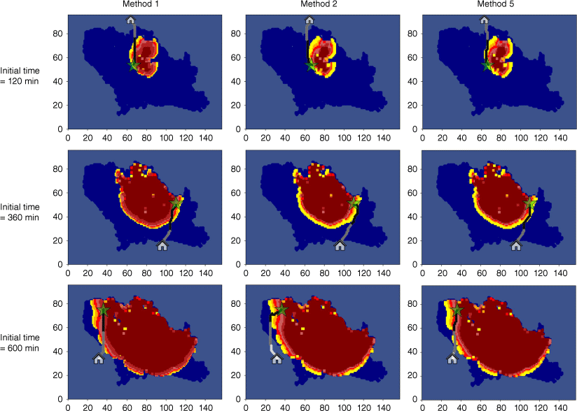
The real fire named MALT was simulated and used as a basis to validate the final improved model (Method 5) proposed in this paper again. The initial location of the fire was chosen at the 120th, 360th, and 600th minute of the fire. The starting point is set closer to the fire, and the endpoint is set outside the burned area of the entire fire. Compare and verify Method 5 with Methods 1 and 2 again, and the results of the escape route and corresponding evaluation indicators in Fig. A1 and Table A1:
| Initial time (min) | Ttotal | MOSLocal avg | MOSLocal min | |||||||
|---|---|---|---|---|---|---|---|---|---|---|
| Method 1 | Method 2 | Method 5 | Method 1 | Method 2 | Method 5 | Method 1 | Method 2 | Method 5 | ||
| 120 | 19.94 | 21.33 | 20.73 | 25.27 | 60 | 47.33 | 10.4 | 60 | 40.83 | |
| 360 | 19.45 | 22.13 | 20 | 22.73 | 45.97 | 39.72 | 6.97 | 39.74 | 32.58 | |
| 600 | 24.35 | 31.53 | 26.34 | 7.89 | 32.68 | 16.7 | −1.64 | 12.23 | 11.12 | |
Method 5 (the final improved model) has much higher security than Method 1 (the traditional method). When compared with Method 2 (the first improved model), it can effectively shorten the total travel time while ensuring a good margin of safety. This proves that planning an escape route can comprehensively and balance the time and safety of the route.