

Examining dispatching practices for Interagency Hotshot Crews to reduce seasonal travel distance and manage fatigue
Erin J. Belval A D , David E. Calkin B , Yu Wei A , Crystal S. Stonesifer B , Matthew P. Thompson C and Alex Masarie AA Department of Forest and Rangeland Stewardship, Warner College of Natural Resources, Colorado State University, Fort Collins, CO 80526, USA.
B USDA Forest Service, Rocky Mountain Research Station, 800 E Beckwith Avenue, Missoula, MT 59801, USA.
C USDA Forest Service, Rocky Mountain Research Station, 240 W Prospect Road, Fort Collins, CO 80526, USA.
D Corresponding author. Email: erin.belval@colostate.edu
International Journal of Wildland Fire 27(9) 569-580 https://doi.org/10.1071/WF17163
Submitted: 31 October 2017 Accepted: 27 June 2018 Published: 23 July 2018
Journal compilation © IAWF 2018 Open Access CC BY-NC-ND
Abstract
Interagency Hotshot Crews (IHCs) are a crucial firefighting suppression resource in the United States. These crews travel substantial distances each year and work long and arduous assignments that can cause accumulated fatigue. Current dispatching practices for these crews are supposed to send the closest resource while adhering to existing fatigue-management policies. In this research, we designed a simulation process that repeatedly implements an optimisation model to assign crews to suppression requests. This study examines the potential effects of using an optimisation approach to shorten seasonal crew travel distances and mitigate fatigue. We also examine the potential benefits of coordinating crew-dispatch decisions to meet multiple requests. Results indicate there is substantial room for improvement in reducing travel distances while still balancing crew fatigue; coordinating crew dispatching for multiple requests can increase the assignment efficiency, particularly when both fatigue mitigation and travel distances are jointly optimised. This research indicates implementing an optimisation model for dispatching IHCs is promising.
Additional keywords: fire fighters: management, fire management: modelling, fire suppression, safety.
Introduction
Dispatching wildland-fire-suppression resources in the United States is an important and complex task, particularly during periods of high fire activity. The existing dispatch system in the US is a complex web of disparate local, regional and national systems and resources – including people, crews, equipment, aircraft and supplies – that respond to demand across a range of jurisdictions. Certain fire-suppression resources available for national-level response are used for large fire-suppression needs and supplement resources in areas of the country experiencing extreme fire activity. The main goal of dispatching these resources is to efficiently send them to where they are needed most. However, issues such as minimising travel distance and mitigating fatigue can complicate dispatching efforts. In addition, during times of elevated resource scarcity, when there are not enough resources to respond to all requests from fire managers, prioritising assignments across fires plays a role in the dispatching decision process.
Here we focus on the dispatching of Type 1 Interagency Hotshot Crews (IHCs). ‘Type 1’ crews are the most highly trained firefighting crews. In a recent survey of US Forest Service fire managers, the field of respondents identified Type 1 crews as the single most important resource in both direct and indirect attack efforts; most respondents also identified Type 1 crews as scarce (Stonesifer et al. 2017). IHCs are a subset of these crews that are specifically designated as national resources and are governed by interagency standards (NIFC 2017a). With between 105 and 120 teams operating each summer, these highly trained crews respond to a high level of national-scale demand (NIFC 2016). Each crew comprises 18–22 firefighters based out of a single location. These crews travel around the country together, typically travelling in two to four ‘crew buggies’ that are equipped with most of the equipment they need. IHCs are highly sought after by the Incident Management Teams that manage large fires, and each year some IHC requests go unfilled due to limited supply.
Owing to high demand and limited supply, IHCs log an extensive number of work hours each season as they move around the country responding to requests during a fire season; many of those hours involve highly strenuous and mentally taxing activities, often in intense heat. Cuddy and Ruby (2011) describe how the combination of fatigue and heat can lead to elevated likelihood of heat exhaustion, in spite of increased levels of hydration. In a review of related literature, Aisbett et al. (2012) highlight that sleep restriction, heat and smoke affect physical and mental performance of fire responders, which places them at increased risk in a demanding work environment. Another important issue for IHCs is managing accumulated fatigue. Although fatigue from a typical single shift of IHC work can be mitigated through adequate rest and recovery, serious physical and mental health impacts can be attributed to accumulated or chronic fatigue, resulting from an extended period of physical or mental taxation combined with inadequate recovery periods (Missoula Technology and Development Center (MTDC) 2002). The MTDC found that chronic fatigue may perpetuate risk factors because fatigued workers may behave carelessly, tolerate greater errors or become inattentive. These are concerns for fire responders both working on the fireline and while in transit.
Policies do exist to mitigate both short-term and accumulated fatigue. For example, the 2-to-1 work-to-rest ratio is an important policy aimed at reducing the impacts of short-term fatigue. Policy dictates that personnel are provided a minimum of 1 h of sleep or rest for every 2 h of work each day, and that shifts exceeding 16 h should be rare (NWCG 2016). Another primary policy aimed at mitigating the effects of fatigue is the ‘14-day rule’ (NIFC 2017a); fire personnel may work for up to 14 days, but then must have at least a 2-day break. Certain exceptions to this are allowed, which may result in fire responders working up to 21 continuous days in unusual circumstances. Some regions of the country do implement ‘rotations’ for out-of-region assignments, which prioritise fire responders leaving on out-of-region assignments on a rotating basis (e.g. Rocky Mountain Coordinating Group 2017). If an out-of-region assignment occurs while a crew is at the top of the rotation, then that crew is sent on that assignment regardless of distance to the incident. Although this may help mitigate fatigue, it may also contribute to issues related to excessive travel. National dispatch protocol currently relies chiefly upon the 14-day rule and regional rotations to account for fatigue in dispatching decisions, with some effect from the 2-to-1 work-to-rest guidelines affecting short-term resource availability. Other considerations specifically aimed at mitigating accumulated fatigue are not currently part of official national-dispatching protocol.
IHCs travel significant distances; in 2016, IHCs drove nearly 5.2 × 10⁶ miles (~8.4 × 10⁶ km) (L. Money, pers. comm., 2017). IHCs, like many other firefighting crews, tend to prefer to drive to incidents. Because they are highly self-sufficient, IHCs generally bring all the equipment and supplies they need to each incident in their crew carriers (also called ‘buggies’ or ‘crummies’) so that they are ready to quickly perform a variety of fire-suppression tasks, and also so that they are able to support their own needs while camped out on the fire line.
The written policies guiding the dispatching of IHCs indicate that they should be dispatched according to the ‘closest forces and total mobility concepts’ (NIFC 2017b), i.e. the closest resource should be dispatched provided that this does not hinder the capacity to ‘move, position, and utilise established forces to meet existing and anticipated fire protection needs nationwide’ (NWCG 2018). Effectively implementing this policy, however, is a multiagency challenge, and different agencies and geographic regions have their own internal policies and procedures that complicate efficiency in dispatching. The US Forest Service recently included all employees involved in fire-suppression activities in a series of ‘Life First’ safety-engagement sessions (Tidwell 2016). Through this, fire responders and managers noted that excessive driving occurs more frequently than necessary, indicating that current dispatching practices may not be following the ‘closest resource’ policy. This is concerning for several reasons. First, any time fire responders are on the road they are exposed to travel hazards. Although the risk associated with driving may seem small, millions of miles add up to significant exposure; 17.6% of wildland fire response fatalities reported by NIFC from 2006 to 2016 were associated with vehicle accidents (NIFC 2017c). Second, travel is expensive, as it includes costs from vehicle use, salaries for time on the road, hotels and meals. Third, if crews are spending their time on the road, they are not spending time engaged in fire-suppression activities, potentially leading to missed suppression opportunities.
IHCs are designated as national resources, which means that the National Interagency Coordination Center (NICC) controls dispatch decisions for IHCs on assignment out of their home region. Further, during times of highest suppression resource demand (National Preparedness Levels 4 and 5), the National Multi-Agency Coordination (NMAC) group is formed at NICC to exert full control over all national resource assignments, including IHCs (NICC 2017a, chapter 2). NMAC decisions are informed through a variety of decision-support tools that project such things as forecasted fire-weather and associated potential fire behaviour; however, to our knowledge, no formal decision-support system exists to facilitate efficient resource assignments.
As there are a relatively small number of IHCs in comparison with other wildland firefighting resources and because of their strategic importance and high demand, these crews provide a test case to examine potential impacts related to implementation of specific dispatching policies. Many of the relevant past studies have focussed on seasonal suppression resource dispatching for standard initial response needs (e.g. Haight and Fried 2007; Ntaimo et al. 2012; Lee et al. 2013) at a scale of a single state or national forest. Other studies have focussed on optimally assigning local wildland fire suppression resources to fires for initial response needs; these models used fire characteristics, resource effectiveness characteristics, and resource location to dynamically build an initial response resource package for each fire (Wiitala 1999; Ntaimo et al. 2013; Wei et al. 2015a, 2015b). Wei et al. (2017) tested a mixed-integer program (MIP) model to study Colorado’s fire crew and engine movements between dispatch zones for four fire seasons. None of these past studies have focussed specifically on Type 1 IHCs or suppression-resource dispatching at the national scale, gaps that we attempt to fill here.
In light of the dispatch challenges for IHCs and the level of unnecessary-driving exposure faced by these fire responders, we built an optimisation model that assigns IHCs to requests while balancing travel and fatigue. A seasonal simulation program uses the optimisation model to test the effects of differing dispatch objectives. With this work we aim to explore the potential gains from developing an optimisation model to reduce seasonal IHC driving distance and promote balanced workloads while meeting the seasonal suppression demand. Although the optimisation model we developed is not complex, running this model based on historical data through seasonal simulations provides insight into the effects of different policies. Feedback from fire responders indicates that a simple model is more likely to be operationally adopted.
In our model, travel distance is calculated from the crew’s location to the fire incident according to Google Earth’s national atlas road-network layer. Accumulated fatigue is included in the model by calculating each crew’s total work hours from the preceding 21 days. Using historical data, we run the model to simulate how requests might have been filled over a fire season given different policy preferences; these simulated fire seasons allow us to examine the effect of differing policies on travel distance, trade-offs between travel distance and mitigating fatigue, and the benefits of coordinating crew dispatching across multiple requests.
Methods
Integer programming model formulation
During periods of low fire activity, crews are generally dispatched as requests come in. However, as fire activity increases and crews become scarce, requests may be held and prioritised by the Regional or NMAC groups and then filled simultaneously once or twice per day. Theoretically, holding requests and filling them simultaneously should increase overall efficiency because dispatching has the opportunity to coordinate the assignments of multiple crews to meet the demands for multiple incidents. The trade-off is a longer response time between a request submission and the assignment of a crew to that request. To reflect the possibility of holding requests and to test if such holding of requests increases efficiency of assignments, we assume each fire day can be divided into a sequence of ‘dispatching coordination time windows’ (DCTWs) varying from 1 min to 24 h. IHC requests in each DCTW are tallied using historical incident and dispatch data. Given the requests for crews submitted within each DCTW, we built an integer programming model to optimise the crew assignments to minimise total travel distances and incentivise choosing crews with a smaller workload from the preceding 21 days. This assignment model is run sequentially across DCTWs for a fire season.
The accumulated crew workload from the preceding 21 days is a proxy for accumulated fatigue that is included in the objective function to allow us to examine trade-offs between travel time and fatigue; incentivising the use of crews with less work in the recent past should distribute work more evenly between crews and mitigate fatigue among crews. We chose to use 21 days to match the longest assignment time possible based upon the 14-day rule. We did test other lengths of time (i.e. 14 days, 30 days and season-to-date) and found the implications of the model results to be mostly insensitive to this parameter, even though individual assignments did differ. Only the 21-day results are presented here for clarity and brevity; the other results are available from the authors on request.
The mathematical formulation of the optimisation model is below. The set of decision variables used in the optimisation model is Fc,i,t, which are binary variables used to track whether a crew c is dispatched to fill request i during a DCTW time t. Fc,i,t = 1 means the crew is dispatched to fill the request; otherwise Fc,i,t = 0.
A set of parameters will be exogenously determined before running the integer program (IP) model at each DCTW t. They include dc,i,t, distance from the current location of crew c to the incident associated with request i (or a function of distance to reflect travel time delay before crew c reaches incident i) in DCTW t; hc,t, hours crew c has worked in the 21 days before DCTW t; w, manager’s weight (preference) for a balanced workload across crews as compared with travel distance; ac,i,t = 1 if crew c is available for assignment to request i in DCTW t, 0 otherwise. This parameter is request-specific; for some DCTWs we find in preprocessing that a crew may be available to go to one request but not another (for example, if a crew is prepositioned and therefore would not be made available for travel to assignments outside of some predefined regions).
At each DCTW t the following IP model will be run to optimise the dispatching of available crews to the requests that occurred within the DCTW.
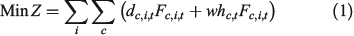


The objective function in Eqn 1 includes terms to minimise the distance a crew travels (dc,i,tFc,i,t; further distances correspond to larger penalties) and to incentivise using crews with fewer hours of work in the preceding 21 days (whc,tFc,i,t). Constraint 2 ensures crews are only sent to requests if they are available for dispatch to that request. Constraint 3 requires one crew be sent to each request. Constraint 4 ensures that each crew can only be sent on a single assignment.
Seasonal simulation model
The integer programing model is embedded in a seasonal simulation model that steps sequentially through all the DCTWs in a fire season. Fig. 1 shows how the simulation is structured. We test varying the length of DCTW in which crew dispatch actions to incidents are simultaneously coordinated and optimised. For each set of requests the program:

|
-
Retrieves each request’s information; specifically, the date of the request and location of the incident.
-
Determines which crews are available and their location (e.g. if they are on season, available and not assigned to another incident or if they are assigned to a preposition request).
-
Calculates travel distance between each crew and the incident using the Google road-network layer.
-
Calculates the total hours each crew worked over the preceding 21 days.
-
Runs the dispatch optimisation model and records the model-selected crew that fills each request.
-
Updates crew availability information based upon filled requests.
The simulation tracks the seasonal travel distances, the hours of work, the total cost of travel and the potential lives lost to travel for each crew (these calculations are discussed in more detail below). We can then compare the travel costs and crew work times of the simulated seasons with optimised assignments to the historical travel costs and work times (estimating costs and times from actual assignments using our model parameters). In addition, we can also examine seasonal workload-to-travel ratios for individual crews to identify spatial and temporal patterns.
Historical request, assignment and availability data used for parameterisation
To parameterise the simulation model, we used requests, assignments and crew availability records from the Resource Ordering and Status System (ROSS) dispatch program (all IHC requests theoretically go through ROSS). Other studies have shown ROSS to be a valuable source of information for examining dispatching and assignments for fire responders and equipment (e.g. Calkin et al. 2014; Belval et al. 2017; Lyon et al. 2017). We only examined filled requests for IHCs; this model is not meant to be used to prioritise which requests should be filled, but rather to fill those already determined to be a priority. Although California has many crews that are qualified as Type 1 crews, several of those crews are not qualified specifically as IHCs; thus, we did not include them in the model, nor did we include the requests that they filled. Some crews were qualified as Type 1 IHCs in some of the years but not others; if they were not qualified for a certain year, they were listed as unavailable for that year. Most IHCs are seasonally employed and are available during the active fire season. Therefore, we only examined requests from 2013 to 2015 that occurred between 1 April and 1 November, a period of time that has historically encompassed the primary fire seasons that tend to occur in each region of the country, and when most seasonal suppression resources and firefighting contracts are on line. We were also able to use the archived crew status data to determine when their seasons started, when their seasons ended, and if there were any periods of extended unavailability during the season.
The ROSS dataset, although a good record of the crews’ assignments, is missing several pieces of information needed by the model. For example, crews can move from one incident directly to another, or they can go from their home base to an incident and then directly back to their home base. The distinction between those two different crew travel paths is not always indicated in ROSS records. We adopt a heuristic to distinguish between the two types of travel. We assume if a crew’s most recent assignment is more than 2 days ago, the crew returned to their home base; otherwise, we assume that the crew was sent directly from incident to incident. This heuristic is consistent with current practice (L. Money, pers. comm., 2017) and allows us to compare travel distances between historical assignments and simulated assignments from the model runs. The distance from each crew’s location to each incident was calculated using an adapted version of Dijkstra’s algorithm (Bertsimas and Tsitsiklis 1997) based on Google Earth’s national atlas road-network layer. This algorithm may be biased towards overestimating travel distances, particularly for short distances, because of a requirement that resources always travel by a highway. Thus, we also calculated the travel distance ‘as-the-crow-flies’ using the Haversine formula (Sinnott 1984). We then ran the model using both sets of distances to see what the effect of the distance calculation was on the final travel distances and costs. As expected, the Haversine distances gave smaller total distances and costs. However, both of the sets of distances showed the same trends. We present the results using Dijkstra’s algorithm in this study as it better reflects driving distances, but results from the other runs are available from the authors upon request.
Another important piece of data not recorded in ROSS is the crew shift length; this often differs from the assignment length, as crews do not work 24 h per day on multi-day assignments; rather, they work assigned shifts that may last from 8 to 16 h and are off for rest at least 8 h each day (NIFC 2017a). Although assignment length is available from ROSS, shift length is not. To calculate the crews’ workload, we developed the following heuristic after discussions with fire responders (L. Money, pers. comm., 2017, and K. Mellott, pers. comm., 2015). If an assignment lasted no longer than 1 day (i.e. the mobilisation date was the same as the demobilisation date), we used the exact number of hours between the mobilisation time and demobilisation time. If the assignment lasted longer than 1 day, a more complicated heuristic was needed, and hours were calculated for each day in the following manner. If the mobilisation time was after 1400 hours then the crew did not work the first day. If the mobilisation time was before 1400 hours then the crew worked 8 h the first day. If the demobilisation time was before 1400 hours, then the crew did not work at all on the last day of the assignment. If the demobilisation time was after 1400 hours, then the crew worked 8 h the last day of the assignment. For the days between the first and last day of assignment, we assumed crews worked 12 h per day.
Preposition requests add an extra layer of complexity to the analysis. Prepositioning requests appear in ROSS when a crew is sent to an area expecting or experiencing a high level of ongoing or anticipated future fire activity. Thus, the preposition places the crew in an area where they are expected to be needed, without assigning them to an actual fire incident. It is important to include these requests because they can substantially affect travel distances and crew availability. A preposition request is filled in the model like any other request. Once a crew is assigned to a preposition request, they become available only for incidents within the same geographic coordination area (GCA) as the preposition request. Fig. 2 shows the GCA boundaries. If assigned to an incident during a preposition, the distance the crew travelled is calculated from the preposition location to the incident location.

|
Although the optimisation program uses travel distance as one of the incentives to prioritise which crews to send, management implications are more readily assessed in the potential cost savings and in the potential expected lives saved by lessening distances travelled. Thus, we calculated the average seasonal cost and the expected number of lives lost per season. Dollar costs included mileage assuming three vehicles per crew (L. Money, pers. comm., 2017) at US$0.535 per vehicle mile (US$0.332 per vehicle km) using the 2017 fiscal year General Services Administration (GSA) mileage per diem rate (GSA 2017), and a base hourly salary rate for each of the 20 crew members assuming 50 miles h−1 and no stops. Travel costs associated with crew salary were calculated assuming an ‘average’ IHCA. We expect these estimates to be conservative as we did not include per-diem costs, hotel costs, overtime and we assumed that any distance over 2500 miles (~4023 km) would be a flight with a fixed cost of $200 per crew member plus 8-h salary. For statistical estimates on potential lives saved, we used 1.12 lives per 100 million vehicle-miles (~1.6 × 10⁸ km) travelled as per the National Highway Traffic Safety Administration (NHTSA) 2016 report (NHTSA 2016). This is also likely conservative, as each IHC vehicle will typically have more people (usually 5–10 persons per vehicle) than the average vehicle on the road. As with travel costs, any trip over 2500 miles (~4023 km) was assumed to be a flight and we assumed zero lives lost associated with that trip, another conservative estimate.
Our model does not have any constraints to force the assignments to conform to the 14-day rule. We considered adding such constraints. However, resources are often assigned to fires without knowing how long the assignment will last. Because the 14-day rule is an important policy, a crew may be assigned to a multiple-day assignment that is terminated exactly when they hit 14 days of work; i.e. the assignment length ends up being tailored to match the crew’s availability. We were limited by the historical assignment lengths and did not want to make assumptions about which assignments might have been shortened (or lengthened) due to adherence to the 14-day rule. Thus, we assumed that it is more realistic to allow for violations of the 14-day rule than to force the model to anticipate assignment lengths, which allows for more flexibility in dispatching than reducing crew availability artificially. To examine how well the model assignments conform to the current 14-day dispatching policy, the simulation model tracks the number of times an assignment violates the 14-day rule; if a crew was sent to an assignment that resulted in them working longer than 14 days without a 2-day break, that assignment was counted as a single violation. We also observed how many violations occurred in the historical data as a baseline comparison.
We hypothesise that certain crews might have a particularly high historical workload and also be heavily assigned in the simulated seasons because of their proximity to the fires. In addition, we wanted to explore the possibilities that some GCAs might have crews with particularly high workloads for years in which they are particularly busy. Thus, the simulation model also tracks each crew’s workload-to-travel distance ratio for each simulated season and for seasons using historical assignments.
We used requests from 2013, 2014 and 2015 from ROSS, only examining requests occurring during the fire season in the US. Each model run consisted of filling the requests for a single year with a specific workload weight and DCTW for simultaneously filling requests. We systematically varied the workload weights, testing 10 weights between 0 and 1000 crew-miles per crew-hour (resulting in testing weights of 0, 111, 222, 333, … 1000 crew-miles per crew-hour)B; 1 crew-hour would be the equivalent of one crew working for 1 h and 1 crew-mile would be the equivalent of one crew travelling 1 mile. A weight of 0 crew-miles per crew-hour indicates we are optimising only travel distance and not considering prior workload; as the weights increase we are placing a higher priority on sending crews with lower prior workloads in comparison with minimising travel distance. We varied the length of the DCTW for each year using DCTWs of 1 min, 1 h, 4 h, 12 h and 24 h. We can then compare the model-suggested national scale dispatching decisions with the historically recorded assignment decisions across each fire season using seasonal travel distances, costs and potential lives lost. We examined the effects of fatigue mitigation by looking at how assigned workloads are distributed across crews. We also examined how well the model results conformed to current fatigue mitigation policy by recording how often crews were assigned to requests that violated the 14-day rule. Lastly, we examined how historical crew usage patterns compare with simulated usage patterns using workload-to-travel ratios to see if any crews or geographic areas see particularly high or low usage and to examine how the simulated usage compares with usage during historical fire seasons.
Results
Fig. 3 shows the total distance travelled for all crews for each of the runs with workload weights up to 600 crew-miles per crew-hour. Regardless of which DCTW length is used, the trend is the same; low values of weights on prior workload result in significantly lower total crew travel distances. The model runs show that seasonal travel distances with the most opportunity for improvement occurred in 2015, which was also a more demanding fire year than 2013 and 2014 (NICC 2017b) so this indicates that travel costs may be more receptive to improvement in busier fire seasons. This could be because the dispatching decisions during a busy fire year are more complex. Table 1 translates crew travel distances into costs and loss-of-life potential.

|

|
Fig. 3 also shows the differences in simulated travel distances for differing DCTW lengths. At low workload weights, the total difference in cost between different DCTWs is nearly imperceptible. However, at higher workload weights, holding requests for longer timeframes can have a significant effect on travel distances. At a lower workload weight, the travel distance is the highest priority and the impact of DCTW is low. However, at a higher workload weight, the travel distance is a lower priority. Thus, when the DCTW is shorter, there is not much room for the travel distance to be optimised; alternatively, longer DCTWs provide the model with more opportunities to optimise travel distance. Holding requests for a few hours to provide more efficient dispatching may be reasonable when sending crews to large fire or preposition assignments, although it would not likely be reasonable when crews are dispatched to initial response assignments when hours of delay may result in increased probability that a fire will escape. Holding requests for 24, 12, 4 and 1 h resulted in a maximum of 38, 25, 16 and 11 requests respectively being filled simultaneously. Filling requests as they come in with a DCTW of 1 min resulted in a maximum of nine requests in a single DCTW. Each of the optimisation program runs was solved by CPLEX (IBM ILOG CPLEX Optimization Studio, provided by IBM; https://www.ibm.com/products/ilog-cplex-optimization-studio) in less than a second on a Hewlett-Packard ZBook laptop running Windows 10 with 16 GB of RAM. Each yearly simulation ran in under 2 min on the same laptop.
Although IHCs can be used as initial response resources, much of their travel occurs when they are travelling to ongoing large fires. A difference of 1 or 2 h is unlikely to matter to the large fire management team (although reducing overall drive times is still valuable in reducing travel costs and risks to crews). However, crews must not drive for more than 12 h day−1; after 12 h of driving significant additional costs are incurred as hotel costs, additional per-diem costs and an overnight delay are added to their travel. We used a heuristic (assuming a 64.4 km h−1 travel speed) to translate travel distances into travel time and calculated the number of requests for which the crew could arrive in less than 12 h. We found that using a larger DCTW can reduce the number of trips that exceed 12 h (see Fig. 4). However, if we want to use higher weights to balance crew workloads, we would have to accept a substantially lower number of trips with less than 12-h travel time (Fig. 4).

|
An example set of our results is in Fig. 5 which shows four of the workload distributions across crews for model runs in 2013, 2014 and 2015 using a 4-h DCTW (Fig. 5).The columns of graphs correspond to different simulation scenarios; the leftmost column shows the historical workload distribution, the three middle columns show the workload distribution if requests had been filled using a workload weight of 0, 111 and 222 crew-miles per crew-hour, from left to right respectively. The rightmost column shows the standard deviation of the workload distributions corresponding to five tested workload weights from 0 to 444; the horizontal dotted line shows the standard deviation of workload according to the historical assignments. When the workload weight is close to zero, the seasonal crew workload is less balanced than historical. However, even at a workload weight as low as 111 the workload is as balanced as the historical assignments, and at 222 crew-miles per crew-hour the workload is more evenly spread across crews than historical. Looking back at Fig. 3 we can observe that at a workload weight of 111 crew-miles per crew-hour (indicated by the vertical dotted line) there is still significant room for improvement in travel costs. Thus, these results indicate that when an optimisation model is used it is possible obtain a workload distribution that is comparable to historical values while significantly reducing travel distances.

|
The number of 14-day violations for each run and for historical records are shown by year in Fig. 6. Increasing the DCTW does not appear to have much of an effect on 14-day violations. The graphs do show that fewer violations are associated with higher workload weights, although the decreasing number of 14-day violations is negligible above the workload weight of 222 crew-miles per crew-hour. The existence of some 14-day rule violations is not surprising, as the model did not include any constraints to prevent them. However, even without such constraints, the number of 14-day rule violations is not substantially higher than historical for workload weights above 222 and, in some cases, is even below historical. The runs for 2013 always show higher than historical numbers of violations; the runs for 2014 and 2015 show similar or lower than historical violations. This may be because 2013 was a lower fire activity year, thus fire managers could limit 14-day rule violations, but since our model does not have any explicit constraint or goal for 14-day rule violations, it did not do the same.

|
The workload-to-travel ratios allow us to identify regions in which crews travel disproportionally high and low distances given their workloads. We are most interested in identifying regions with crews that are travelling long distances to work comparatively less (i.e. a low ratio; low travel efficiency), or those that are travelling short distances and working more (i.e. a high ratio; high travel efficiency). By comparing the average ratio of historical crew workloads to crew travel distances between GCAs (Table 2), we found that the historical workload-to-travel ratio averages correspond with historical regional-fire activity. For example, in 2013 the region with the highest workload-to-travel distance ratio was Southern California (OSCC), which was also the only region that experienced above average acres burned (138% of their 10-year average) in the same year (NICC 2017b). Similarly, in 2014, the only regions to observe higher than average area burned were Northern California (ONCC; 152% of their 10-year annual average) and the Northwest (NWC; 214% of their 10-year annual average) (NICC 2017b); both regions were in the top three regions with the highest workload-to-travel ratio. These patterns often held in the simulated fire seasons using our model as well, although the workload-to-travel ratio variability between regions was moderated in the simulation runs with higher weights on workload. For example, in the 2014 simulated runs optimised with a 4-h DCTW, crews from ONCC and NWC both show high workload-to-travel ratios for all runs when workload weight is less than 222 crew-miles per crew-hour. As the workload weight increases, the workload-to-travel ratio decreased for both regions and the discrepancy between regions decreases. These changes reflect overall longer travel distances paired with more highly balanced workloads between crews from different regions.

|
Discussion and conclusion
The test cases in this research demonstrated some major strengths of using an optimisation model for dispatching IHCs. By running this model across multiple fire seasons and adhering to consistent dispatching policies across regions, we found overall reduced travel distance, better fatigue mitigation and increased workload equity. The discrepancy between our estimates on travel distance using historical data and the travel distances produced by using the simulation and optimisation model with low workload weights indicate that IHCs may not have historically been dispatched by a strict ‘closest resource first’ policy. Thus, if reducing travel distances is important to policy makers, there is likely substantial room for improvement, even while mitigating crew fatigue. Besides reducing travel times, adopting a centralised dispatch organisation would likely reduce local and regional control over IHCs, which is a significant change from current practices, particularly during quieter times in the fire season.
The results also indicate that as crew fatigue becomes more of a concern to managers, holding requests within a wider DCTW and coordinating the dispatch for multiple assignments can have substantial benefits. During times of significant fire resource scarcity, this has been practiced, as IHC requests have been submitted throughout a day and have then been processed by NMAC after they determined the highest priority assignments (NICC 2017a). Therefore, our test results suggest that this type of practice may have led to reductions in travel and fatigue; however, the current IHC assignment process could become more transparent and efficient with the support of structured decision support models such as the one developed here. Enhanced application of optimisation models could play an important role in ensuring improved outcomes.
This model used the crews’ workload in the preceding 21 days to balance crew workload to mitigate fatigue, which also helps ensure equal work opportunities among crews. Workload equity is likely a concern for seasonal fire crew personnel who may rely upon fire season income to provide the bulk of their yearly earnings. The results from this study show that it is possible to both reduce travel distance and equalise workload between crews.
Of the years that we examined, 2015 had the highest levels of fire activity (NICC 2017b), and it was also the year where our simulated fire seasons showed the most improvement in reducing crew travel distance. Thus, using a centralised point of dispatching and ensuring that the policy of ‘closest first’ is followed may provide the largest gains in years when IHCs are in particularly high demand. Such years of high demand are also typically years with greater fire suppression expenditure; thus, in such years, savings on travel distance and associated cost would be particularly important. In addition, mitigating fatigue becomes increasingly important during busier fire seasons. We may observe less adherence to the ‘closest-first’ policy during busy years in part due to drawdown restrictions, which limit how many IHCs are allowed to be outside their home region during times of high regional preparedness levels. Such drawdown constraints are intended to keep IHCs in areas of high fire activity so as to be more responsive as fires emerge. Our results do not directly address responsiveness, but if indeed IHCs held for drawdown were providing a higher responsiveness due to the drawdown acting as a preposition, then we’d expect to actually see shorter driving distances as the IHC would respond to emerging fires nearby. The increased room for decreasing travel distance in our results during busy years may indicate that the drawdown restrictions are not having their intended effect.
When we examined historical average workload-to-travel ratios by region, we found substantial variation between regions. We would expect crews in regions that experienced higher fire activity to have higher workload-to-travel ratios; such crews are simply closer to many incidents and thus do not need to travel as far. Thus, this variation is not inherently concerning. However, we can also observe that we can achieve a similar distribution of workload-to-travel ratios with substantially less travel using workload weights of 200–400 crew-miles per crew-hour. In addition, some of the simulated results using workload weights between 200 and 400 crew-miles per crew-hour show substantially less variation, with improved assignment equity between crews. However, this equity comes at the cost of the crews closest to the heavy fire activity travelling further and working less. It is an open policy question of what balance of fatigue mitigation and travel distance is appropriate.
Although the test cases in this study show that running the current optimisation model through a fire season can substantially benefit the dispatching process by reducing the total crew travel distance and balancing crew workload, it can still be enhanced to further improve the IHC dispatching efficiency. For example, the current model dispatches IHCs only based on the known requests from incidents; with better prediction of future fire activity and resource demand, the model can be more proactive by holding an IHC in a region expecting significant fire activity and sending an IHC from a region less likely to have significant fire activity. We expect research in predicting future suppression resource demand could be easily integrated into our current modelling system to improve nationwide IHC dispatching (see e.g. Preisler et al. 2016; Wei et al. 2017). In addition, the model could be altered to identify particularly urgent requests (i.e. with a closing ‘due date’) and send the closest crews to those requests before filling other requests.
Using a centralised decision system for dispatching IHCs would reduce local control of these resources and could be unpopular as restrictions such as drawdown and out-of-area crew rotations are common within regions (e.g. RMCG 2017). The applications of such dispatch systems could initially identify and recommend crews with the highest score (closest resource with lowest weighted recent workload) to dispatch personnel, which may facilitate adoption without the perceived restriction of decision-maker control.
Future research using a modified version of this model might examine the effect of local dispatch policies, such as drawdown restrictions. Such research would be quite valuable to determine the policy effects and help guide both local and national decision makers. Further, the model and research presented in this paper provide a basis for future work examining dispatch practices related to other types of widely used firefighting resources, such as wildland engines and other crews, as dispatching practices for those resources differs from the IHCs.
This research did not address responsiveness in the classic initial response fashion (i.e. looking to see if decreased travel time allows for more requests for IHCs to be filled). IHCs are a limited resource often serving ongoing large fires. During periods of high fire activity nearly every crew is out on assignment or on their required 2 days of rest. Decreasing driving time is currently a primary concern in the US. The decreased travel distance would likely increase the amount of time that crews can be used on a fire and fatigue recovery.
The national systems of dispatch and resource allocation in the US have not been widely studied, and are not consistently guided by the best available science and models, instead relying upon expert judgement. Modelling efforts introduced here build on a growing body of research aimed at improving the use and allocation of suppression resources across space and time. In the interest of improved efficiency and minimising risk associated with excessive travel and seasonal fatigue, a more thorough understanding of the underlying dispatch structures could be facilitated by in-depth development of more advanced operations research models, which might be implemented to meet clear resource allocation objectives in the future.
Conflicts of interest
The authors declare that they have no conflicts of interest.
Acknowledgements
This research was supported by Joint Venture Agreement 14-JV-11221636–029 between Colorado State University and the USDA Forest Service Rocky Mountain Research Station. The authors thank Larry Money, who helped with data verification and provided us with valuable insights from the field regarding their needs. Thanks also go to Shephard Crim who helped provide the ROSS data for this study. We also thank the two anonymous reviewers and the Associate Editor whose suggestions and comments enhanced this paper.
References
Aisbett B, Wolkow A, Sprajcer M, Ferguson SA (2012) Awake, smoky, and hot: providing an evidence-base for managing the risks associated with occupational stressors encountered by wildland firefighters. Applied Ergonomics 43, 916–925.| Awake, smoky, and hot: providing an evidence-base for managing the risks associated with occupational stressors encountered by wildland firefighters.Crossref | GoogleScholarGoogle Scholar |
Belval EJ, Wei Y, Calkin DE, Stonesifer CS, Thompson MP, Tipton JR (2017) Studying interregional wildland fire engine assignments for large fire suppression. International Journal of Wildland Fire 26, 642–653.
| Studying interregional wildland fire engine assignments for large fire suppression.Crossref | GoogleScholarGoogle Scholar |
Bertsimas D, Tsitsiklis JN (1997) ‘Introduction to Linear Optimization.’ (Athena Scientific and Dynamic Ideas, LLC: Belmot, MA, USA)
Calkin DE, Stonesifer CS, Thompson MP, McHugh CW (2014) Large airtanker use and outcomes in suppressing wildland fires in the United States. International Journal of Wildland Fire 23, 259–271.
| Large airtanker use and outcomes in suppressing wildland fires in the United States.Crossref | GoogleScholarGoogle Scholar |
Cuddy JS, Ruby BC (2011) High work output combined with high ambient temperatures caused heat exhaustion in a wildland firefighter despite high fluid intake. Wilderness & Environmental Medicine 22, 122–125.
| High work output combined with high ambient temperatures caused heat exhaustion in a wildland firefighter despite high fluid intake.Crossref | GoogleScholarGoogle Scholar |
GSA (2017) Privately owned vehicle (POV) mileage reimbursement rates. (General Services Administration) Available at https://www.gsa.gov/travel/plan-book/transportation-airfare-rates-pov-rates-etc/privately-owned-vehicle-pov-mileage-reimbursement-rates [Verified 12 September 2017]
Haight RG, Fried JS (2007) Deploying wildland fire suppression resources with a scenario-based standard response model. INFOR 45, 31–39.
| Deploying wildland fire suppression resources with a scenario-based standard response model.Crossref | GoogleScholarGoogle Scholar |
Lee Y, Fried JS, Albers HJ, Haight RG (2013) Deploying initial attack resources for wildfire suppression: spatial coordination, budget constraints, and capacity constraints. Canadian Journal of Forest Research 43, 56–65.
| Deploying initial attack resources for wildfire suppression: spatial coordination, budget constraints, and capacity constraints.Crossref | GoogleScholarGoogle Scholar |
Lyon KM, Huber-Stearns HR, Moseley C, Bone C, Mosurinjohn NA (2017) Sharing contracted resources for fire suppression: engine dispatch in the Northwestern United States. International Journal of Wildland Fire 26, 113–121.
| Sharing contracted resources for fire suppression: engine dispatch in the Northwestern United States.Crossref | GoogleScholarGoogle Scholar |
Missoula Technology and Development Center (2002) Wildland Firefighter Health & Safety Report 5, Spring 2002. (Missoula, MT, USA)
NHTSA (2016) Traffic safety facts research note: 2015 motor vehicle crashes: overview. August 2016. National Highway Traffic Safety Administration’s National Center for Statistics and Analysis. (Washington, DC, USA)
NICC (2016) ‘Standards for Interagency Hotshot Crew Operations.’ (National Interagency Coordination Center: Boise, ID, USA)
NICC (2017a) 2017 National Mobilization Guide. (National Interagency Coordination Center: Boise, ID, USA)
NICC (2017b) 2017 Wildland Fire Summary and Statistics Annual Reports 2013–2015. NICC, Boise ID. Available at https://www.nifc.gov/fireInfo/fireInfo_statistics.html [Verified 12 September 2017]
NWCG (2016a) ‘NWCG Interagency Business Management Handbook.’ (National Wildfire Coordinating Group: Boise, ID, USA)
NIFC (2017b) About NIFC. Available at https://www.nifc.gov/aboutNIFC/about_main.html [Verified Sept 12, 2017]
NIFC (2017c) Wildland fire fatalities by year. (National Wildfire Coordinating Group: Boise, ID, USA) Available at https://www.nifc.gov/safety/safety_documents/Fatalities-by-Year.pdf [Verified 12 September 2017]
Ntaimo L, Arrubla JAG, Stripling C, Young J, Spencer T (2012) A stochastic programming standard response model for wildfire initial attack planning. Canadian Journal of Forest Research 42, 987–1001.
| A stochastic programming standard response model for wildfire initial attack planning.Crossref | GoogleScholarGoogle Scholar |
Ntaimo L, Arrubla JAG, Gang J, Stripling C, Young J, Spencer T (2013) A simulation and stochastic integer programming approach to wildfire initial attack planning. Forest Science 59, 105–117.
| A simulation and stochastic integer programming approach to wildfire initial attack planning.Crossref | GoogleScholarGoogle Scholar |
NWCG (2018) Total Mobility. Available at https://www.nwcg.gov/term/glossary/total-mobility [Verified 10 February 2018]
OPM (2017) 2017 General schedule (GS) locality pay tables. (Office of Personnel Management) Available at https://www.opm.gov/policy-data-oversight/pay-leave/salaries-wages/2017/general-schedule/ [Verified 12 September 2017]
Preisler HK, Riley KL, Stonesifer CS, Calkin DE, Jolly M (2016) Near-term probabilistic forecast of significant wildfire events for the Western United States. International Journal of Wildland Fire 25, 1169–1180.
| Near-term probabilistic forecast of significant wildfire events for the Western United States.Crossref | GoogleScholarGoogle Scholar |
RMCG (2017) ‘Rocky Mountain Area Interagency Mobilization Guide 2017.’ (Rocky Mountain Coordinating Group, Rocky Mountain Area Coordination Center: Lakewood CO, USA)
Sinnott RM (1984) Virtues of the Haversine. Sky and Telescope 68, 158
Stonesifer CS, Calkin DE, Hand MS (2017) Federal fire managers’ perceptions of the importance, scarcity and substitutability of suppression resources. International Journal of Wildland Fire 26, 598–603.
| Federal fire managers’ perceptions of the importance, scarcity and substitutability of suppression resources.Crossref | GoogleScholarGoogle Scholar |
Tidwell TL. (2016) Life First. Message From the Chief, sent to all FS Employees Nov 28, 2016.
Wei Y, Bevers M, Belval EJ, Bird B (2015a) A chance-constrained programming model to allocate wildfire initial attack resources for a fire season. Forest Science 61, 278–288.
| A chance-constrained programming model to allocate wildfire initial attack resources for a fire season.Crossref | GoogleScholarGoogle Scholar |
Wei Y, Bevers M, Belval EJ (2015b) Designing seasonal initial attack resource deployment and dispatch rules using a two-stage stochastic programming procedure. Forest Science 61, 1021–1032.
| Designing seasonal initial attack resource deployment and dispatch rules using a two-stage stochastic programming procedure.Crossref | GoogleScholarGoogle Scholar |
Wei Y, Belval EJ, Thompson ME, Calkin DE, Stonesifer CS (2017) A simulation and optimisation procedure to model daily suppression resource transfers during a fire season in Colorado. International Journal of Wildland Fire 26, 630–641.
| A simulation and optimisation procedure to model daily suppression resource transfers during a fire season in Colorado.Crossref | GoogleScholarGoogle Scholar |
Wiitala MR (1999) A dynamic programming approach to determining optimal forest wildfire initial attack responses. In ‘Fire Economics, Planning, and Policy: Bottom Lines’. pp. 115–123. (USDA Forest Service: Berkeley, CA, USA)
A There are several sets of possible combinations of personnel that could create a Type 1 IHC; we used average salaries computed from the Office of Personnel Management (OPM) salary schedule (OPM 2017) for two different possible configurations and then took the average of those configurations. More detail is available from the authors upon request.
B The conversion rate from crew-miles per crew-hour to crew-km per crew- hour is 1.61. Thus, the weights used in crew-km per hour are 0, 178.6, 357.3, 535.9, 1609.3 crew-km per crew-hour.