
Analysis of Nanoconfined Protein Dielectric Signals Using Charged Amino Acid Network Models
Lorenza Pacini A B D , Laetitia Bourgeat A C D , Anatoli Serghei C E and Claire Lesieur A B E
A B E
A AMPERE, CNRS, University of Lyon, 69622, Lyon, France.
B Institut Rhônalpin des Systèmes Complexes, IXXI-ENS-Lyon, 69007, Lyon, France.
C IMP, CNRS, University of Lyon, 69622, Lyon, France.
D These authors contributed equally to this work.
E Corresponding authors. Email: anatoli.serghei@univ-lyon1.fr; claire.lesieur@ens-lyon.fr
Australian Journal of Chemistry 73(8) 803-812 https://doi.org/10.1071/CH19502
Submitted: 5 October 2019 Accepted: 27 February 2020 Published: 19 May 2020
Journal Compilation © CSIRO 2020 Open Access CC BY
Abstract
Protein slow motions involving collective molecular fluctuations on the timescale of microseconds to seconds are difficult to measure and not well understood despite being essential to sustain protein folding and protein function. Broadband dielectric spectroscopy (BDS) is one of the most powerful experimental techniques to monitor, over a broad frequency and temperature range, the molecular dynamics of soft matter through the orientational polarisation of permanent dipole moments that are generated by the chemical structure and morphological organisation of matter. Its typical frequency range goes from 107 Hz down to 10−3 Hz, being thus suitable for investigations on slow motions in proteins. Moreover, BDS has the advantage of providing direct experimental access to molecular fluctuations taking place on different length-scales, from local to cooperative dipolar motions. The unfolding of the cholera toxin B pentamer (CtxB5) after thermal treatment for 3 h at 80°C is investigated by BDS under nanoconfined and dehydrated conditions. From the X-ray structure of the toxin pentamer, network-based models are used to infer the toxin dipoles present in the native state and to compute their stability and dielectric properties. Network analyses highlight three domains with distinct dielectric and stability properties that support a model where the toxin unfolds into three conformations after the treatment at 80°C. This novel integrative approach offers some perspective into the investigation of the relation between local perturbations (e.g. mutation, thermal treatment) and larger scale protein conformational changes. It might help ranking protein sequence variants according to their respective scale of dynamics perturbations.
Introduction
Protein dynamics covers multiple spatiotemporal scale processes, including slow motions (microsecond to second), which are not much understood because they are difficult to measure, even though they are underlying protein folding and protein functions.[1–3]
Fast motions (femtosecond to nanosecond) concern local atomic motions (vibration, amino acid side chain motions) and are measured by ultra-fast techniques such as ultra-fast NMR spectroscopy, femtosecond simulated Raman spectroscopy, ultra fast transient Infra Red spectroscopy, or ultra resolution X-ray crystallography and X-ray laser.[4–13] Molecular dynamics (MD) simulations have atomic resolution and can now also cover motions up to a millisecond thanks to the ANTON super computer.[1] However, MD simulations at high resolution are limited in terms of size and it remains hard to assess motions slower than the microsecond range.[14,15]
Slow motions concern the collective motions of many atoms within areas of large size such as secondary and tertiary structural elements (microsecond to millisecond) up to domains or chain (millisecond to second).[3] The slow fluctuation dynamics is monitored by lower spatial resolution techniques such as atomic force microscopy (AFM) or fluorescence spectroscopy (e.g. Förster resonance energy transfer, FRET), where the detailed MDs are generally lost.[16–18] The slow motions are also investigated with network models and integrative approaches combining experimental and multiple theoretical approaches.[19–30] They are particularly successful in monitoring the slow motions involved in protein assembly and pore formation.[28,31–33]
Broadband dielectric spectroscopy (BDS), although not often used on proteins, can monitor protein MDs in the frequency range from 1 Hz to 106 Hz where the slow motions from microseconds to seconds involved in protein folding and protein functions take place.[34–37] The advantage of BDS is the capacity to characterise dipole features both at the local scale (dipole environment) with the temperature at maximum signal, and at a larger scale through fluctuations of collective motions exhibiting a characteristic relaxation tau (τ), defined as the inverse of the frequency. However, as for other biophysics methods such as fluorescence spectroscopy, the measurement is performed at the macroscopic scale where responses come from the bulk composed of many protein and solvent molecules containing many dipoles.
To overcome some of these limits, the dynamics of the cholera toxin B pentamer (CtxB5) was measured by BDS after different thermal treatments, but under nanoconfined and dehydrated conditions.[37] Thus, no bulk water contributed to the dielectric signal and attograms (considering a density of ~1 g cm−3, 1 attogram is ~10 nm × 10 nm × 10 nm) of matter were probed, approaching the characteristic dimension of one protein.[37] The nanoconfinement, initially developed to analyse attograms (1 attogram = 10−18 g) and zeptograms (1 zeptogram = 10−21 g) of matter, allows one to investigate the dielectric behaviour of matter on a length-scale comparable with the molecular dimensions.[38,39] In our study, the BDS signal was found to probe protein conformations that arise from the toxin thermal unfolding.[37] Based on knowledge on the scale of protein dynamics and on toxin unfolding mechanisms, a model of the toxin thermal unfolding monitored by BDS was proposed where two non-native pentamers and toxin assembly intermediates were captured.
Nevertheless, because the sample was a mixture of protein, phosphate buffered saline (PBS), and adsorbed water, the global dielectric signal was not de-convoluted in terms of distinct dipolar relaxation.
Here, we use network-based models to infer the protein dipoles present in the native toxin pentamer and network based analyses to show that, consistently with our model, the toxin interfaces are distinguishable dielectrically and thermally.
Results and Discussion
We have recently shown that the dielectric signals of CtxB5 measured by BDS in nanoconfined and dehydrated conditions evolved with the thermal treatments of the toxin at 60, 100, 140, and 180°C, probing for the toxin thermal unfolding.[37] However, because the protein sample was a mixture of three compounds – the protein, phosphate buffer saline (PBS), and protein adsorbed-water – it was impossible to analyse the global dielectric signals in terms of individual dipolar relaxations. In fact, understanding the individual contribution of each compound and how the individual signals combine together to give rise to the global signal is intractable.
Instead, we proposed a model of the thermal toxin unfolding where the global dielectric signal was interpreted based on the knowledge on protein dynamics from MD simulations and from experimental investigations of protein assembly and disassembly under macroscopic conditions where non-native pentamers and CtxB assembly intermediates were identified.[39–42] Protein assembly can be described by two mechanisms, the induced fit mechanism where the protein monomer folds before assembling and the fly-casting mechanism where the folding and assembling are concomitant.[40,43–45] Protein disassembly involves transitions from native oligomers to either folded monomers or non-native oligomers.[46–49] In the model, the three distinct MDs detected by BDS, referred to as MD1, MD2 and MD3, were assigned to two different non-native pentamers (MD1 and MD3) and to toxin assembly intermediates (MD2), suggesting that the dielectric signal probed the toxin interfaces.[37]
Here, we use network-based models to describe the dipoles present at the toxin interface and to test this hypothesis.
As the sample is composed of three compounds, water, salt (PBS), and protein, the first issue is to determine whether the MDs are the water, PBS, and protein respective individual dielectric signals.
BDS Combined with Nanoconfinement
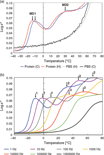
First, the dielectric behaviour of the toxin is investigated after three hours incubation at 80°C during which the toxin unfolds. Toxin samples are deposited in the nanomembrane and the dielectric loss ϵ′ is measured by BDS (see Experimental). After thermal treatment for 3 h at 80°C, the dielectric loss ϵ′ is measured as a function of temperature going from 80 to −80°C (cooling) and from –80 back to 80°C (heating). The dielectric loss ϵ′ of the samples during the cooling ramp is shown in Fig. 1 for frequencies ranging from 1 to 106 Hz.
|
The cooling and heating curves show similar dielectric signals demonstrating that the proteins under study are stabilised in a state where no bulk water is present anymore (i.e. no more water evaporation) (Fig. 1a). In the previous study, it was shown that the protein sample contains adsorbed water.[37] As observed in our previous study, the protein spectra can be described by three relaxation processes, which give rise to three peaks in the spectra of the dielectric loss (Fig. 1b). The PBS buffer control shows only a conductivity contribution under the same conditions indicating that the signal in the protein sample is protein dependent (Fig. 1a).
The absence of MD for the PBS buffer control indicates that the individual dielectric signals of the water, the salt (PBS), and the protein are non-additive and the Havrialiak–Negami functions cannot be applied to de-convolute the global signal. The three MDs are not the respective individual dielectric signal of the water, the salt, and the protein but their coupled responses.
The second issue is to determine how many sets of dipoles are associated with the three MDs.
The main relaxation process, referred to as MD1 (molecular dynamics peak 1), is identified by a narrow peak and it is the fastest, with a maximum dielectric loss ϵ′ at temperature θmax equal to −14°C at 1 Hz. MD1 is detected for frequencies from 1 to 105 Hz. The second relaxation process, referred to as MD2, has a broader peak and is slower with θmax equal to 30°C at 1 Hz. The broadness of MD2 suggests a relaxation process associated with a more heterogeneous population of average toxin conformations compared with the average toxin conformations associated with the narrower MD1 peak. This leads to the assumption that MD2 is associated with more thermally perturbed toxin conformations than MD1 and CtxB assembly intermediates (tetramer, trimer, and dimer). Unfolding leads to loss of atomic interactions such that MD2, which is detected only at low frequencies from 1 to 102 Hz and therefore exhibits fluctuations of larger-scale atomic motions (domain or chain) than the faster frequencies of 103 Hz and above observed in MD1, is in a more unfolded state than MD1.[3] The third relaxation process, referred to as MD3, has a narrow peak as MD1 but appears only at frequencies higher than 100 Hz indicating the loss of the dipoles detected at low frequencies in MD1 and so a more unfolded state than the average conformations associated with MD1. Because MD3 has fast motion dipoles and smaller-scale motions than the slow dipoles detected in MD2, it is in a less unfolded state than MD2. Thus as reported previously for thermal treatments at higher temperatures, three unfolding toxin intermediates can be associated with the BDS signal, two non-native pentamers, MD1 and MD3, and toxin assembly intermediates with MD2.[37]
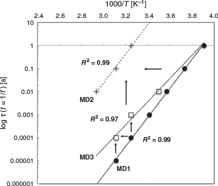
For the three MDs, the positions of the maximum dielectric signals (θmax) shift to higher temperatures with increasing frequencies. The temperature dependencies of the relaxation times tau (τ), which are the inverse of the frequency (τ = 1/f), can be followed by plotting τ against the temperature at the maximum signal for the respective frequency (Fig. 2).
|
The relaxation times follow an Arrhenius linear temperature dependency indicating that dipoles fluctuating at different frequencies are independent from one another (see Experimental). This is true for the three relaxation processes. The relaxation times become longer from MD1 to MD3 to MD2 (Fig. 2, vertical arrows).
Longer relaxation times mean dipole fluctuations involving larger collective motions consistently with more advanced stage of the toxin unfolding. The temperatures at maximum signals (θmax) shift to higher temperatures (lower 1000/T) for dipoles with similar relaxation times from MD1 to MD3 and for MD1 to MD2 (Fig. 2, horizontal arrows). This shift means that thermal unfolding also leads to changes in the vicinity of dipoles (changes in the temperature at maximum signals) with no impact on the dipole relaxation time (no change in tau) or that different sets of dipoles (changes in the temperature at maximum signals) with similar fluctuation scales (no change in tau) are probed.
MD1 and MD2 have dipoles with slow motions but not with the same temperatures at maximum signals, indicating that two different sets of dipoles are detected in MD1 and MD2. This is confirmed by the loss of the MD1 slow fluctuations dipoles in MD3, interpreted as an intermediate unfolding stage between MD1 and MD2. The set of dipoles with fast motions in MD1 is detected as well in MD3 but with slightly slower motions indicating larger collective motions probably due to further unfolding (Fig. 2, vertical arrows). This set of dipoles is no more detected in the MD2, probably because the area unfolded further and the resulting motions fall out of the measured frequency range. Native dipole fluctuations are unlikely to be detected as they fall within time scales equal or below nanoseconds.[1,3] According to other experiments and MD simulations, slow motions (millisecond to second) are large domains and chains, while fast motions (microsecond to millisecond) involve smaller areas such as secondary and tertiary structural elements.[1,3]
In summary the MD1 is associated with two sets of dipoles, one with slow fluctuations and the other one with fast fluctuations. The set with fast motions is also detected in MD3 and a third set of dipoles with slow motions is detected in MD2. The dipoles with fast motions in MD1 and MD3 could be detected in MD2 but with slower motions due to a more advanced toxin unfolding. However, because the motions in MD2 are a thousand times slower it is unlikely that such larger unfolding leads to no change in the local environment of the dipoles (no change in the temperature at maximum signals). It is more reasonable to consider that MD2 is associated with a third set of dipoles which has similar temperatures at maximum signals than the set of dipoles with fast fluctuations in MD1 and MD3. Thus, two sets of dipoles with slow motions are detected and one set with fast motions.
Network Based Models
The BDS data indicate that three sets of dipolar relaxations are detected and the model of the toxin thermal unfolding assumes that MD1 and MD3 are non-native pentamers while MD2 is associated with assembly intermediates, implying that the toxin interfaces are probed by the BDS signal.
Hence, for the model to be valid, the toxin interfaces need to be dielectrically detectable, thermally sensitive, and be composed of three different sets of dipolar relaxations with distinct thermal sensitivity.
To investigate such a possibility, network-based models are used to study the toxin interfaces in terms of stability and dielectric features. The steps to build the different networks are schematised in Fig. S1 (Supplementary Material).
Modelling Interactions in the Toxin Interfaces and Ranking Interface Stability
An intermolecular interaction network, referred to as a 4D-network, was built based on the X-ray structure of the toxin native pentamer to describe the toxin interface (see Experimental). The nodes of the network are amino acids which belong to different chains and which can be connected because they have at least one pair of atoms within a threshold distance of 5 Å. The links are weighted according to the exact number of pairs of atoms, one per chain that are within a threshold distance of 5 Å. The 4D-network models intermolecular atomic and amino acid interactions, namely the interactions involved in the toxin interface. As an approximation of the interface stability, the number of amino acid and atomic interactions involved in the 4D-network are computed.
The toxin interface is rather complex and made of three physically distinct domains, I1, I2, and I3 (Fig. 3).

|
For simplicity, in Fig. 3, I1, I2, and I3 sub-domain interfaces are shown on a trimer of the toxin instead of a pentamer involving the chains D, E, and F. I1 is the N-terminal sub-domain interface domain of the toxin, it involves residues 1 to 12 of chain E and interacts with two sub-domains on the adjacent chain F. The residues 1 to 3 of chain E interact with residues 92 and 93 on chain F and constitute a weak patch (I1a) of the sub-domain interface I1 with only 5 amino acid pairs and 46 atomic interactions (Table 1). The sub-domain interface I1b is made of residues 1 to 12 of chain E and residues 28 to 39 of chain F and constitutes a moderate interface composed of 19 amino acid pairs and 137 atomic interactions (Table 1). I2 constitutes the main sub-domain β-interface of the toxin and is composed of the β-strand number 3 (residues 25 to 39) and the β-strand number 6 (residues 96 to 103). The residues 25 to 32 of chain E interact with the residues 88 and 96 to 103 on chain D (I2a) and constitute a strong interface (I2a) with 26 amino acid pairs and 198 atomic interactions (Table 1). The residues 28 to 39 of chain E interact with some of the residues 58 to 68 of the central helix (residues 58 to 81) of chain D, constituting a moderate interface (I2b) with 19 amino acid pairs and 136 atomic interactions (Table 1). Finally, there is a weak interface patch (I2c) involving interactions between residues 101 to 103 of chain E and residues 73, 76–77 on the adjacent chain F with only 5 amino acid pairs and 22 atomic interactions (Table 1). I3 is the central α-helix sub-domain interface, composed of residues 58 to 81 of chain E interacting with residues 58 to 81 on the adjacent chains D and F. This is a tri-partite interface as it involves interactions between chain E and F as well as between chain E and D (Fig. 3), but it still constitutes a single interface with two ‘sticky’ moieties. The central α-helix sub-domain interface I3 is the strongest interface with 24 amino acid pairs and 214 atomic interactions (Table 1).

|
Based on the number of atomic and amino acid interactions, the toxin stability of the sub-domain interfaces can be ranked as follows: I1a and I2c are the weakest, I1b and I2b are moderate, and I2a and I3 are the strongest (Table 1).
Dielectric Properties of the Toxin Interface and Ranking
In order to assess the dielectric properties of the toxin interface, an intermolecular charged amino acid network and an intermolecular induced charged amino acid network were built (see Experimental). The former is referred to as the 4D-charged network and the latter as the 4D induced charged network. The 4D-charged network is a sub-network of the 4D-network where only charged amino acids are retained (see Experimental). The pairs of charged residues are called ionic dipoles. The 4D induced charged network is initially built as the 4D-charged network but the non-charged amino acid neighbours in the 4D-network of the nodes are added. The pairs of non-charged residues are called induced dipoles. The construction of the different networks is schematised in Fig. S1 (Supplementary Material).
The choice of these two types of networks to model the dipoles in the native state of the toxin pentamer and infer dipoles which are detected by BDS is supported by the following reasons. First, protein structures and protein dynamics rely on non-specific hydrophobic interactions (van der Waals) and specific electrostatic interactions (e.g. salt bridges, charged-dipoles), the latter are contributing more to the dielectric signal as they involve Coulomb forces. Moreover, the electrostatic interactions are key to the folding and the stability of a protein and are believed to play a major role in the protein thermal stability.[43] Second, charged residues and their proximal neighbours are the major constituents of the electrostatic interactions in proteins.[50] Third, the electrostatic interactions in protein structures depend on the pH and the salt conditions, such that considering interactions between charged residues as an approximation of the coupling between protein, water, and salt (PBS) dipoles is relevant.[50] Because the pH is 6.9 and based on disassembly and reassembly pH-dependency studies, the N- and C-terminals, lysine and arginine residues are considered protonated while glutamic and aspartic acids are considered deprotonated and hence participating in the 4D-charged network.[40,46,51–53]
Based on the 4D-charged network and the 4D-induced charged network, the dielectric properties of the different interface sub-domains are deduced (Table 1) (Fig. 3). I1a and I2c are dielectrically invisible and weakly visible, respectively, as they have no charged residues but I2c has two induced dipoles. I1b and I2b have two ionic dipoles (pair of charged residues) and some induced dipoles (charged–non charged pairs). I2a is invisible dielectrically as it has no charged residues but it can be detected through the induced dipoles in the environment of the charged residue Glu29 (Table 1). I3 is the strongest dielectric interface domain of the toxin with 13 ionic dipoles and 5 induced dipoles.
Dielectric and Stability Features of the Toxin Interfaces and BDS Signal Interpretation
Based on the dielectric and stability features of the toxin interface, we can draw the following conclusions on the dipoles that are participating to the BDS signal. The I1a and I2c domains are the weakest and ranked as the most temperature-sensitive domains but they cannot be detected by BDS or only weakly through induced dipoles (Table 1). The thermal perturbation of I1a will be detected when I1b is thermally perturbed as well through the ionic dipoles T1–R35 and E11–R35 (Table 1) (Fig. 4). Likewise, the thermal perturbation of the I2c domain will be detected via the perturbation of the induced dipoles and the ionic dipoles involving Glu29 when I2a and I2b are thermally disturbed (Table 1) (Fig. 4). Because I1b is a moderate interface in terms of amino acid and atomic interactions compared with I2a, I1b unfolding is likely to occur before the unfolding of I2a and so I1b is associated with the slow motion dipoles detected in MD1 but lost in MD3. It follows that I2a and I2b are associated with the fast motion dipoles observed in MD1 and MD3. The slow dipoles of MD2 are associated with the I3 interface sub-domain as this domain has the strongest stability and the highest number of ionic dipoles and would be detected in the most unfolded stage of the toxin. In MD2, the toxin conformations would have lost the I1 and I2 sub-domain interfaces, their dipoles being no more detected by BDS such that the chain dissociation would occur as only an I3 destabilised interface remains (slow motion = large fluctuation).

|
The thermal unfolding perturbation and the dipoles detected in MD1 are schematized in Fig. 4.
The weak interfaces unfold, leading to the perturbation of the I1 N-terminal interface detected by dipoles with slow motions and to the perturbation of the I2 β-interface detected by dipoles with fast motions. The dipoles detected in MD3 and MD2 are shown on the 4D-charged network and the 4D-induced charged network, respectively on Fig. 5. The interface I2 further unfolds in MD3 where the dipoles involving the residues Glu29 and Glu36 and the residues Lys63 and Arg67 on the adjacent chains are detected. In MD2, the N-terminal I1 interface and the I2 interface are unfolded and not detected anymore, while only dipoles from the central helix I3 interface are still detected.

|
Conclusion
This novel network approach to analyse dielectric signals, using network-based models and infer toxin interface dielectric and stability properties from the X-ray structure, supports the hypothesis that BDS probes the thermal perturbation of the toxin interfaces. The toxin interface is composed of three sub-domains that have distinct dielectric and stability features as expected from the model of the toxin thermal unfolding. Moreover, the scale of the motions detected by the BDS is also in good agreement with the unfolding stage of the toxin: the I1 N-terminal unfolding likely leads to chain motion and the detected slow fluctuations (millisecond to second), in MD2 only the I3 sub domain interface is connecting two chains which is likely to lead to chain dissociation and the detected slow fluctuations, the fast motions involving the I2 interface perturbation is a smaller scale fluctuation involving secondary structure element motions.
Our study is not an exhaustive investigation of the dipoles involved in the BDS signal, and intramolecular contributions are probably also taking place, a possibility that can be explored in the future using charged intramolecular networks instead. Nevertheless, the results allow the pinpointing of some residues potentially important for the toxin unfolding and detected dielectrically, such as the charged pair R35–E11 in the I1 interface, the charged dipoles E29–(A97, A98, I99, S100) and R73–M101 in the I2 interface and several charged pairs K63–E66, R67–D70, and D70–R73 in the central α-helix. The results also suggest that the I3 interface is the most stable and most dielectrically detectable interface in the toxin. Thus, based on the results, toxin mutants can be proposed to test the roles of these amino acids both in the dielectric signals and in the toxin thermal unfolding. This integrative approach could also be used to investigate protein sequence variants and rank them according to dynamics perturbations. The network analysis combined with the experimental molecular dynamics measured by BDS in nanoconfined conditions offers a powerful approach to investigate the relation between local perturbations and global protein conformational changes.
Experimental
BDS and Nanoconfinement
Materials
Lyophilized cholera toxin B pentamer purchased from Sigma Aldrich (C9903) was diluted in phosphate buffered saline (PBS; 10 mM sodium phosphate, 150 mM sodium chloride, pH 7.4) at a final concentration of 2.6 mg mL−1. This bulk toxin preparation was aliquoted and kept at −20°C, and thawed and frozen two times at most, when used for the dielectric measurements. Concentrated PBS solutions were purchased from BIOSOLVE and diluted 10 times in distilled water to prepare the PBS used in the bulk toxin solution. In addition, the PBS solution was filtered by 22 μm filters to limit impurity contamination. The aluminium oxide (AAO) films on Al were purchased from InRedox. The AAO membrane dimensions were 10 mm × 10 mm, and they contained nanopores of 40 nm diameter and 10 µm length, with 12 % porosity. The AAO membrane containing the nanopores is referred to as the nanomembrane. Before use, the nanomembranes were plasma-treated for 20 min to remove organic impurities.
Methods
Protein sample preparation. For the dielectric measurement, a protein sample at 0.025 mg mL−1 was used. This protein sample was prepared by diluting 2 μL of the bulk toxin solution at 2.6 mg mL−1 in 204 μL of deionised water (final pH 6.9). Since the bulk protein is prepared in PBS, the sample for the dielectric measurement contains protein, deionised water, and PBS. A 200 μL drop of sample was deposited on the nanomembrane using the drop technique, and then heated at 50°C (323 K) for 15 min to evaporate the bulk water and allow proteins to enter the pores. The sample was cooled to 30°C (303 K) for 5 min with a speed of 2 K min−1, placed between two Al electrodes of 7 and 40 mm diameter, respectively, and placed in the cell holder for measurement. The procedure was the same for the control samples.
Dielectric measurements. The dielectric measurements were performed on a broadband dielectric spectrometer Novocontrol Alpha analyser over a frequency range from 1 to 106 Hz and a temperature range from –80 (193) to 80°C (353 K). The temperature ramps were carried out at a rate of 2 K min−1 and a voltage of 0.2 V was applied. The dielectric loss ϵ′, the imaginary part of the complex dielectric permittivity, was measured as a function of temperature at different frequencies. For the temperature control, a flow of pure nitrogen gas was used in a closed cryostat, providing water-free and oxygen-free experimental conditions. The sample was first heated to 80°C (353 K) for 3 h, and to −80°C (193 K) (cooling, C) and maintained for 30 min before being heated back to 80°C (heating, H). A cycle was composed of the cooling (C) and the heating (H) temperature ramp. The curves of the cooling and heating signals were very similar for the protein sample (Fig. 1a). This demonstrates that the proteins under study were stabilised in a state where no bulk water is present anymore and where the amount of adsorbed water is stabilised as well. It also shows that the protein remains in a steady-state across the measurement and undergoes thermal unfolding mainly during the 3 h incubation time. The PBS buffer control showed no molecular dynamics and only had conductivity after treatment at 80°C (Fig. 1a). The dielectric signals are therefore from the protein.
Dielectric data. The temperature dependence of the relaxation processes was modelled by an Arrhenius equation expressed as Eqn 1:[34,35]

where τ is the relaxation time, τ0 the relaxation time at high temperatures, T the temperature, EA the activation energy, and kB the Boltzmann constant.[45]
Control experiments. The dielectric response of the empty nanomembrane was measured for 10 min at 60°C and from 60 to −80°C to control that no dielectric dispersions were detected. The dielectric response of nanopores filled with a 200 μL drop of deionised water was measured for 10 min at 60°C and from 60 to −80°C to control that the deionised water used to prepare the sample show no dielectric dispersions too. Finally, the dielectric response of nanopores filled with a 200 μL drop of PBS buffer control was measured following a complete temperature ramp experiment as for the protein sample. The PBS buffer control was prepared with 2 μL of PBS diluted in 204 μL of deionised water (no protein was added). This concentration was equivalent to the concentration used to prepare and measure the protein sample. This control experiment was carried out to investigate the dielectric response of PBS mixed with deionised water in the same conditions as the protein.
To make sure the toxin was in a native state when a dielectric experiment is performed, the toxin pentameric state was checked by Trp-fluorescence beforehand.[45] The sample could not be recovered from the nanopores after the BDS experiment so it was not possible to control the state of the toxin after.
Network Based Models
Intermolecular Amino Acid Network
The toxin interfaces were modelled by a network of the amino acids that belong to different chains and had at least one pair of atoms within a 5 Å distance, so-called hotspots.[24] The amino acid network (AAN) of the whole pentamer was built first and the intermolecular amino acid network was generated after by selecting only intermolecular interactions. The networks were created using the Python Biograph module, available at https://github.com/rodogi/biographs, or directly with the script available at https://github.com/lorpac/network_vmd. Briefly this was done using the atomic coordinates of the toxin structure (PDB: 1EEI) freely available from the RCSB website (https://www.rcsb.org/) and computing intermolecular atomic distances between amino acids that belong to different chains (nodes). Hotspots were linked when their respective atoms were close enough for a chemical interaction using 5 Å distance as a threshold. Such spatial networks based on Euclidian distances between nodes are classically used in proteins to infer atomic and amino acid interactions intractable otherwise due to the size of the system.[2,22,54] From the intermolecular amino acid network of the toxin, simple network measures such as number of hotspot pairs, number of atomic interactions, number of charged amino acid pairs, and number of charged dipole pairs within the interfaces were computed. A charged dipole pair was a charged amino acid interacting with a polar or hydrophobic amino acid. The intermolecular amino acid networks were referred to as a 4D-network for simplicity, 4D corresponds to the quaternary structure of proteins, namely the number of chains present in a protein oligomer.
Intermolecular Charged Amino Acid Network
The intermolecular charged amino acid networks were sub-networks of the intermolecular amino acid networks where only charged amino acids are kept as nodes of the network. The charged amino acid networks model the Coulomb interactions with charged–charged interactions within the toxin interface and were used to analyse the protein dielectric signals which result from such interactions. The intermolecular charged amino acid networks were referred to as the 4D-charged network for simplicity. The orientation of the dipoles was not taken into account in the model although it could cancel out the contribution to the dielectric signal of some of the dipoles considered in the model when dipoles of equal strength had opposite orientation. Nevertheless, the amino acid neighbourhood was sufficiently anisotropic for this to be unlikely, making the approximation locally reasonable. The isoelectric point (pI) of the toxin pentamer was around pH 5.6 such that at pH 6.9 the global charge was negative and a global dipolar moment was expected, consistent with having a dielectric signal. It also supported the approximation at the global scale of the entire protein.
Intermolecular Induced Charged Amino Acid Network
The intermolecular induced charged amino acid network was as the intermolecular charged amino acid network but with the addition of the non-charged amino acids located in the chemical vicinity of the charged hotspots. This network models the Coulomb interactions as well as the ion-dipole interactions with the charged non-charged amino acid pairs, present at the toxin interface. The intermolecular induced charged amino acid networks were referred to as 4D-induced charged network for simplicity.
Mathematically, if the network of all amino acid interactions is represented by a graph G(V, E) with set of nodes V (Vertices) and set of edges (E), then the 4D-network is represented by a graph  with nodes

and edges

The 4D-charged network is then represented by a graph  with nodes

and edges

and the 4D-induced charged network is represented by a graph  with nodes

and edges

The construction of the networks is shown in Fig. S1 (Supplementary Material).
Network Generation and Representation
All networks were generated by manipulating the amino acid network of the toxin using the Python package NetworkX.[46] Two-dimensional network representations were produced using the Gephi software[48] and three-dimensional network representations were produced using the Python scripts available at https://github.com/lorpac/network_vmd and visualised with the VMD software.[49] For simplicity, the toxin pentamer having a central symmetry, only links between nodes involved in the interfaces between chain E and D and between chain E and F are represented.
Supplementary Material
A schematic of the network construction flow is available on the Journal’s website.
Author contributions
LB and LP performed research and analysed data; AS designed research, analysed data, and wrote the manuscript; CL designed research, analysed data, and wrote the manuscript.
Conflicts of Interest
The authors declare no conflicts of interest.
Acknowledgements
The authors thank the Interdisciplinary Mission of the CNRS for funding (MITI, Defi ‘Instrumentations aux limites’ ATTOGRAM).
References
[1] K. Lindorff-Larsen, S. Piana, R. O. Dror, D. E. Shaw, Science 2011, 334, 517.| Crossref | GoogleScholarGoogle Scholar | 22034434PubMed |
[2] L. Vuillon, C. Lesieur, Curr. Opin. Struct. Biol. 2015, 31, 1.
| Crossref | GoogleScholarGoogle Scholar | 25791607PubMed |
[3] V. Munoz, M. Cerminara, Biochem. J. 2016, 473, 2545.
| Crossref | GoogleScholarGoogle Scholar | 27574021PubMed |
[4] T. R. Barends, L. Foucar, A. Ardevol, K. Nass, A. Aquila, S. Botha, R. B. Doak, K. Falahati, E. Hartmann, M. Hilpert, M. Heinz, M. C. Hoffmann, J. Köfinger, J. E. Koglin, G. Kovacsova, M. Liang, D. Milathianaki, H. T. Lemke, J. Reinstein, C. M. Roome, R. L. Shoeman, G. J. Williams, I. Burghardt, G. Hummer, S. Boutet, I. Schlichting, Science 2015, 350, 445.
| Crossref | GoogleScholarGoogle Scholar | 26359336PubMed |
[5] M. Levantino, G. Schiro, H. T. Lemke, G. Cottone, J. M. Glownia, D. Zhu, M. Chollet, H. Ihee, A. Cupane, M. Cammarata, Nat. Commun. 2015, 6, 6772.
| Crossref | GoogleScholarGoogle Scholar | 25832715PubMed |
[6] E. Mizohata, T. Nakane, Y. Fukuda, E. Nango, S. Iwata, Biophys. Rev. 2018, 10, 209.
| Crossref | GoogleScholarGoogle Scholar | 29196935PubMed |
[7] J. R. Stagno, Y. Liu, Y. R. Bhandari, C. E. Conrad, S. Panja, M. Swain, L. Fan, G. Nelson, C. Li, D. R. Wendel, T. A. White, J. D. Coe, M. O. Wiedorn, J. Knoska, D. Oberthuer, R. A. Tuckey, P. Yu, M. Dyba, S. G. Tarasov, U. Weierstall, T. D. Grant, C. D. Schwieters, J. Zhang, A. R. Ferré-D’Amaré, P. Fromme, D. E. Draper, M. Liang, M. S. Hunter, S. Boutet, K. Tan, X. Zuo, X. Ji, A. Barty, N. A. Zatsepin, H. N. Chapman, J. C. H. Spence, S. A. Woodson, Y.-X. Wang, Nature 2017, 541, 242.
| Crossref | GoogleScholarGoogle Scholar | 27841871PubMed |
[8] J. Herbst, K. Heyne, R. Diller, Science 2002, 297, 822.
| Crossref | GoogleScholarGoogle Scholar | 12161649PubMed |
[9] C. Kolano, J. Helbing, M. Kozinski, W. Sander, P. Hamm, Nature 2006, 444, 469.
| Crossref | GoogleScholarGoogle Scholar | 17122853PubMed |
[10] Y. Mizutani, T. Kitagawa, Chem. Rec. 2001, 1, 258.
| Crossref | GoogleScholarGoogle Scholar | 11895123PubMed |
[11] C. Fang, R. R. Frontiera, R. Tran, R. A. Mathies, Nature 2009, 462, 200.
| Crossref | GoogleScholarGoogle Scholar | 19907490PubMed |
[12] R. Schneider, M. Blackledge, M. R. Jensen, Curr. Opin. Struct. Biol. 2019, 54, 10.
| Crossref | GoogleScholarGoogle Scholar | 30316104PubMed |
[13] E. W. Findsen, T. W. Scott, M. R. Chance, J. M. Friedman, M. R. Ondrias, J. Am. Chem. Soc. 1985, 107, 3355.
| Crossref | GoogleScholarGoogle Scholar |
[14] C. Lesieur, K. Schulten, Curr. Opin. Struct. Biol. 2015, 31, v.
| Crossref | GoogleScholarGoogle Scholar | 26055121PubMed |
[15] J. R. Perilla, B. C. Goh, C. K. Cassidy, B. Liu, R. C. Bernardi, T. Rudack, H. Yu, Z. Wu, K. Schulten, Curr. Opin. Struct. Biol. 2015, 31, 64.
| Crossref | GoogleScholarGoogle Scholar | 25845770PubMed |
[16] G. R. Heath, S. Scheuring, Nat. Commun. 2018, 9, 4983.
| Crossref | GoogleScholarGoogle Scholar | 30478320PubMed |
[17] B. Hellenkamp, P. Wortmann, F. Kandzia, M. Zacharias, T. Hugel, Nat. Methods 2017, 14, 174.
| Crossref | GoogleScholarGoogle Scholar | 27918541PubMed |
[18] A. Soranno, A. Holla, F. Dingfelder, D. Nettels, D. E. Makarov, B. Schuler, Proc. Natl. Acad. Sci. USA 2017, 114, E1833.
| Crossref | GoogleScholarGoogle Scholar | 28223518PubMed |
[19] D. M. Leitner, T. Yamato, Mapping Energy Transport Networks in Proteins, Vol. 31 2018 (Wiley Online Library: Hoboken, NJ).
[20] J. Liu, R. Nussinov, PLOS Comput. Biol. 2016, 12, e1004966.
| Crossref | GoogleScholarGoogle Scholar | 27814363PubMed |
[21] A. N. Naganathan, Curr. Opin. Struct. Biol. 2019, 54, 1.
| Crossref | GoogleScholarGoogle Scholar | 30268910PubMed |
[22] L. Di Paola, A. Giuliani, Curr. Opin. Struct. Biol. 2015, 31, 43.
| Crossref | GoogleScholarGoogle Scholar | 25796032PubMed |
[23] C.-B. Li, H. Yang, T. Komatsuzaki, Proc. Natl. Acad. Sci. USA 2008, 105, 536.
| Crossref | GoogleScholarGoogle Scholar | 18178627PubMed |
[24] M. Achoch, R. Dorantes-Gilardi, C. Wymant, G. Feverati, K. Salamatian, L. Vuillon, C. Lesieur, Phys. Chem. Chem. Phys. 2016, 18, 13770.
| Crossref | GoogleScholarGoogle Scholar | 26688116PubMed |
[25] A. Gheeraert, L. Pacini, V. S. Batista, L. Vuillon, C. Lesieur, I. Rivalta, J. Phys. Chem. B 2019, 123, 3452.
| Crossref | GoogleScholarGoogle Scholar | 30943726PubMed |
[26] E. G. Marklund, J. L. Benesch, Curr. Opin. Struct. Biol. 2019, 54, 50.
| Crossref | GoogleScholarGoogle Scholar | 30743182PubMed |
[27] M. T. Degiacomi, Structure 2019, 27, 1034.
| Crossref | GoogleScholarGoogle Scholar | 31031199PubMed |
[28] A. J. Pak, G. A. Voth, Curr. Opin. Struct. Biol. 2018, 52, 119.
| Crossref | GoogleScholarGoogle Scholar | 30508766PubMed |
[29] H. Van den Bedem, J. S. Fraser, Nat. Methods 2015, 12, 307.
| Crossref | GoogleScholarGoogle Scholar | 25825836PubMed |
[30] M. T. Degiacomi, I. Iacovache, L. Pernot, M. Chami, M. Kudryashev, H. Stahlberg, F. G. van der Goot, M. Dal Peraro, Nat. Chem. Biol. 2013, 9, 623.
| Crossref | GoogleScholarGoogle Scholar | 23912165PubMed |
[31] C. M. Boyd, D. Bubeck, Curr. Opin. Struct. Biol. 2018, 52, 41.
| Crossref | GoogleScholarGoogle Scholar | 30125772PubMed |
[32] E. S. Parsons, G. J. Stanley, A. L. Pyne, A. W. Hodel, A. P. Nievergelt, A. Menny, A. R. Yon, A. Rowley, R. P. Richter, G. E. Fantner, D. Bubeck, B. W. Hoogenboom, Nat. Commun. 2019, 10, 2066.
| Crossref | GoogleScholarGoogle Scholar | 31061395PubMed |
[33] G. Schiro, A. Cupane, E. Vitrano, F. Bruni, J. Phys. Chem. B 2009, 113, 9606.
| Crossref | GoogleScholarGoogle Scholar | 19537774PubMed |
[34] H. Jansson, R. Bergman, J. Swenson, J. Phys. Chem. B 2005, 109, 24134.
| Crossref | GoogleScholarGoogle Scholar | 16375405PubMed |
[35] H. Frauenfelder, G. Chen, J. Berendzen, P. W. Fenimore, H. Jansson, B. H. McMahon, I. R. Stroe, J. Swenson, R. D. Young, Proc. Natl. Acad. Sci. USA 2009, 106, 5129.
| Crossref | GoogleScholarGoogle Scholar | 19251640PubMed |
[36] S. Khodadadi, S. Pawlus, A. P. Sokolov, J. Phys. Chem. B 2008, 112, 14273.
| Crossref | GoogleScholarGoogle Scholar | 18942780PubMed |
[37] L. Bourgeat, A. Serghei, C. Lesieur, Sci. Rep. 2019, 9, 17988.
| Crossref | GoogleScholarGoogle Scholar | 31784681PubMed |
[38] A. Serghei, W. Zhao, D. Miranda, T. P. Russell, Nano Lett. 2013, 13, 577.
| Crossref | GoogleScholarGoogle Scholar | 23323871PubMed |
[39] C. Lesieur, M. J. Cliff, R. Carter, R. F. James, A. R. Clarke, T. R. Hirst, J. Biol. Chem. 2002, 277, 16697.
| Crossref | GoogleScholarGoogle Scholar | 11877421PubMed |
[40] J. Zrimi, A. Ng Ling, E. Giri-Rachman Arifin, G. Feverati, C. Lesieur, PLoS One 2010, 5, e15347.
| Crossref | GoogleScholarGoogle Scholar | 21203571PubMed |
[41] B. Goins, E. Freire, Biochemistry 1988, 27, 2046.
| Crossref | GoogleScholarGoogle Scholar | 3378043PubMed |
[42] V. Bhakuni, D. Xie, E. Freire, Biochemistry 1991, 30, 5055.
| Crossref | GoogleScholarGoogle Scholar | 2036374PubMed |
[43] B. A. Shoemaker, J. J. Portman, P. G. Wolynes, Proc. Natl. Acad. Sci. USA 2000, 97, 8868.
| Crossref | GoogleScholarGoogle Scholar | 10908673PubMed |
[44] K. Luke, M. Perham, P. Wittung-Stafshede, J. Mol. Biol. 2006, 363, 729.
| Crossref | GoogleScholarGoogle Scholar | 16979655PubMed |
[45] L. W. Ruddock, J. J. Coen, C. Cheesman, R. B. Freedman, T. R. Hirst, J. Biol. Chem. 1996, 271, 19118.
| Crossref | GoogleScholarGoogle Scholar | 8702586PubMed |
[46] L. W. Ruddock, S. P. Ruston, S. M. Kelly, N. C. Price, R. B. Freedman, T. R. Hirst, J. Biol. Chem. 1995, 270, 29953.
| Crossref | GoogleScholarGoogle Scholar | 8530395PubMed |
[47] M. N. Blackburn, E. A. Noltmann, Arch. Biochem. Biophys. 1981, 212, 162.
| Crossref | GoogleScholarGoogle Scholar | 7305401PubMed |
[48] K. E. Neet, D. E. Timm, Protein Sci. 1994, 3, 2167.
| Crossref | GoogleScholarGoogle Scholar | 7756976PubMed |
[49] M. Perham, M. Chen, J. Ma, P. Wittung-Stafshede, J. Am. Chem. Soc. 2005, 127, 16402.
| Crossref | GoogleScholarGoogle Scholar | 16305220PubMed |
[50] D. Roberts, R. Keeling, M. Tracka, C. F. Van Der Walle, S. Uddin, J. Warwicker, R. Curtis, Mol. Pharm. 2015, 12, 179.
| Crossref | GoogleScholarGoogle Scholar | 25389571PubMed |
[51] M. De Wolf, G. Van Dessel, A. Lagrou, H. J. Hilderson, W. Dierick, Biochim. Biophys. Acta 1985, 832, 165.
| Crossref | GoogleScholarGoogle Scholar | 4063375PubMed |
[52] M. J. De Wolf, G. A. Van Dessel, A. R. Lagrou, H. J. Hilderson, W. S. Dierick, Biochemistry 1987, 26, 3799.
| Crossref | GoogleScholarGoogle Scholar | 3651415PubMed |
[53] R. Gilardi-Dorantes, L. Bourgeat, L. Pacini, L. Vuillon, C. Lesieur, Phys. Chem. Chem. Phys. 2018, 20, 25399.
[54] J. S. Viloria, M. F. Allega, M. Lambrughi, E. Papaleo, Sci. Rep. 2017, 7, 1.