

A Trip to the Density Functional Theory Zoo: Warnings and Recommendations for the User*
Lars Goerigk A B and Nisha Mehta AA School of Chemistry, The University of Melbourne, Parkville, Vic. 3010, Australia.
B Corresponding author. Email: lars.goerigk@unimelb.edu.au
Australian Journal of Chemistry 72(8) 563-573 https://doi.org/10.1071/CH19023
Submitted: 17 January 2019 Accepted: 9 February 2019 Published: 1 March 2019
Abstract
This account is written for general users of density functional theory (DFT) methods as well as experimental researchers who are new to the field and would like to conduct such calculations. Its main emphasis lies on how to find a way through the confusing ‘zoo’ of DFT by addressing common misconceptions and highlighting those modern methods that should ideally be used in calculations of energetic properties and geometries. A particular focus is on highly popular methods and the important fact that popularity does not imply accuracy. In this context, we present a new analysis of the openly available data published in Swart and co-workers’ famous annual ‘DFT poll’ (http://www.marcelswart.eu/dft-poll/) to demonstrate the existing communication gap between the DFT user and developer communities. We show that despite considerable methodological advances in the field, the perception of some parts of the user community regarding their favourite approaches has changed little. It is hoped that this account makes a contribution towards changing this status and that users are inspired to adjust their current computational protocols to accommodate strategies that are based on proven robustness, accuracy, and efficiency rather than popularity.
Introduction
After Kohn and Sham’s seminal paper in 1965[1] and groundbreaking advancements by others in the 1980s and early 1990s,[2–13] density functional theory (DFT) has become the most frequently applied computational-chemistry technique. It is not only used by specialised computational and theoretical chemists, but thanks to its availability in standard quantum-chemistry software and its relatively easy technical applicability, it is also commonly used by experimentalists to support and theoretically underpin their experimental findings. Many high-impact chemistry papers nowadays rely on DFT-based insights. In fact, phrases such as ‘DFT’ or ‘B3LYP’ have made it into nearly every chemist’s vocabulary. The transforming influence of DFT on the discipline in general can best be seen by the fact that one half of the 1998 Nobel Prize in Chemistry was awarded to Walter Kohn.
However, despite being immensely popular and readily available, it is by far not easy for the user to carry out the right DFT calculation for the right reason. ‘DFT’ is not a simple keyword, but one is faced with hundreds of methods—usually called ‘density functionals’ or ‘density functional approximations’ (DFAs)—and for non-experts it has become increasingly difficult to be up to date and to know which methods to choose and which to avoid. In fact, we are inclined to go that far as to state that there is an increasing gap between the developer and user communities due to the large and ever-growing ‘zoo’ of DFAs. As a consequence, the field is riddled with misconceptions—some of which we will address later—and it is no surprise that many users base their computational strategies on popular and highly cited, albeit older, DFAs, which raises the question whether popularity really implies accuracy. The answer to that question can best be summarised by quoting a paper by Kruse, Goerigk and Grimme from 2012 whose title contained the warning: ‘Why the B3LYP/6-31G* model chemistry should not be used in DFT calculations of molecular thermochemistry’.[14]
Thanks to the generous award of the 2017 Royal Australian Chemical Institute Physical Chemistry Division Lectureship, the first author of this account was able to address a general audience of chemists from over 20 chemistry departments across Australia and New Zealand between August 2017 and March 2018 with a lecture series that carried a similar title to this work. His main goal was to make his own humble contribution towards closing the aforementioned communication gap between developers and users and to inform the latter about the current state of the field. This account is meant to serve as a succinct summary of a large portion of that lecture series. It touches on recent contributions by both others and us with the main focus being on four aspects: the importance of London-dispersion effects, accurate energetic properties, the question of popularity and accuracy, and molecular geometry optimisations. By no means can this manuscript be a complete review of everything that has been achieved in the field. Instead, it is meant to be read by non-experts in the field, mainly researchers who occasionally rely on DFT calculations or who intend to carry out such calculations in the future. We hope that our summary introduces them to the confusing DFT zoo, makes them aware of common traps, and provides practical tips that enable them to make an informed decision before undertaking new computational endeavours.
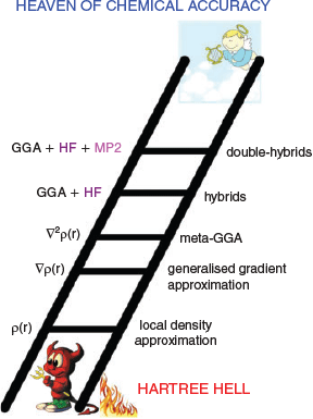
The Jacob’s Ladder Classification of DFT
DFT is an exact theory as shown by Hohenberg and Kohn in 1964.[15] This means the ‘true’ density functional offers a route to the exact solution to the Schrödinger Equation for many-electron systems at a cost that is only a fraction of elaborate wave-function electron-correlation methodologies. However, for all practical purposes the previous statement is not useful, as we do not know what the true functional looks like. Instead, our day-to-day calculations rely on DFAs, each with their individual advantages, disadvantages and inherent errors. To bring order into this chaotic DFT zoo, Perdew and Schmidt introduced the idea to classify each DFA according to its fundamental ‘ingredients’. Based on the nature of those ingredients, the DFA is then assigned to one of five rungs on a ladder.[16] Analogous to the Old Testament, they named the resulting classification the ‘Jacob’s Ladder’ of DFT; Fig. 1 shows a modified and modernised version of this idea. According to the original publication, the ladder connects the ‘Hartree World’ of non-interacting electrons with the heaven of chemical accuracy, with each higher rung promising more accurate results. In later works, the term ‘Hartree Hell’ also appeared (see Fig. 1). From a chemist’s perspective, the latter phrase actually makes sense, as Hartree Theory does not describe the phenomenon of quantum-mechanical exchange between indistinguishable electrons.[17,18] In other words, Hartree Theory violates the Pauli Principle, which is fundamental to chemistry; indeed, a world without the Pauli Principle can be considered as hell for a chemist. The heaven of chemical accuracy represents the exact solution to the Schrödinger Equation. However, for pragmatic reasons most in the computational-chemistry community aspire to the following arbitrary targets to be understood as ‘chemical accuracy’: 1 kcal mol−1 for reaction energies (REs) or barrier heights (BHs), 0.1 kcal mol−1 for noncovalent interaction (NCI) energies, and 0.1 eV for electronic excitation energies.
|
The lowest rung on Jacob’s Ladder is occupied by local density approximation (LDA) functionals. They are based on the uniform electron gas (UEG) idea in which one imagines the entire universe to be filled with a gas of evenly distributed electrons that can move freely within a positively charged background potential that ensures overall charge neutrality.[18–20] In such a model, the electron density ρ is constant and expressions for such a case were derived both for the exchange[21] and electron-correlation[22,23] energy contributions to the total electronic energy. It comes as no surprise that LDA functionals fail for chemical systems because the electron density in a molecule is anything but constant. However, LDA methods now form the foundation for the most commonly used higher-rung DFAs and developers attempted to address the LDA shortcomings with additional corrections. One of those corrections is the generalised gradient approximation (GGA), which is represented by the second rung of Jacob’s Ladder. GGA methods rely not only on the electron density as an input, but also on its gradient ∇ρ. Similarly to LDAs, a GGA energy expression can be divided into an exchange and correlation contribution. Popular representatives for GGAs are the BLYP,[7–9] BP86,[4,5,7] PBE,[11] or B97-D functionals.[24] In 2012, Peverati and Truhlar suggested avoiding the mathematical distinction between exchange and correlation and to use one mathematical expression that encompasses both. The resulting non-separable gradient approximation[25] (NGA) formally also belongs to the second rung on Jacob’s Ladder. The third rung in Fig. 1 takes into account higher-order derivates of ρ, or alternatively the orbital kinetic energy density τ, which involves a sum over squares of the first derivatives of occupied orbitals with respect to spatial coordinates. The resulting methods belong to the class of meta-GGAs/NGAs, with TPSS[26] or M06L[27] being common examples.
The first three rungs are (semi-)local by nature, as they only assess the density at specific points and in their nearest vicinity. Quantum-mechanical exchange, however, is a non-local phenomenon and its accurate treatment with semi-local descriptors is therefore difficult. Fourth-rung functionals solve this problem by replacing some portion of semi-local DFT exchange with conventional Fock exchange,[17,18] which is known from Hartree-Fock (HF) theory. Popular examples of such ‘hybrid’ functionals are BHLYP (also called BH and HLYP),[12] PBE0 (also called PBE1PBE),[28,29] B3LYP,[13,30] or M062X.[31] In the same spirit, Grimme suggested in 2006 to replace parts of semi-local DFT correlation with an orbital-dependent non-local perturbative term, which in practice is identical to what is known as second-order Møller-Plesset perturbation theory (MP2).[32] The first of such ‘double-hybrid’ density functionals (DHDFs) was B2PLYP.[32] More accurate successors were suggested later, for instance Goerigk and Grimme’s PWPB95,[33] Kozuch and Martin’s series of ‘DSD’ functionals,[34–36] and Head-Gordon and co-workers’ ωB97X-2[37] and ωB97M(2).[38] Ref. 39 contains an in-depth review of DHDFs and Ref. 40 provides the most recent overview of DHDF names and performance. Note that Fig. 1 refers only to DHDFs for pragmatic reasons, as they are the currently most practicable representatives for the fifth rung. Perdew and Schmidt originally assigned all methods that rely on virtual (unoccupied) orbitals to that rung. Indeed, we would like to acknowledge recent advancements of other methods in that area, in particular of random-phase approximation (RPA) methods.[41–46]
The hypothesis behind the Jacob’s Ladder of DFT is that higher rungs should deliver better results, something we will address again later. At the same time, the ladder also implies that the higher one climbs, the higher the computational effort is. Indeed, hybrid DFAs are more resource intensive than (meta-)GGAs/NGAs. DHDFs rely on an MP2-like term, and as such they inherit its formal scaling behaviour of O(N5) with N being the system size, such as number of atoms or number of basis functions for the linear combination of atomic orbitals (LCAO) approximation. In comparison, HF (and hybrid DFT) formally scale as O(N4). That being said, specific DHDFs, such as PWPB95, employ techniques to bring down the formal scaling behaviour to O(N4).[47,48] In addition, almost every major DFT code—with one notable exception—makes use of the more than 25 year old resolution-of-the-identity (RI) technique (also referred to as ‘density fitting’) to speed up the evaluation of MP2.[49] Paired with an RI-MP2 algorithm, our group routinely performs DHDF calculations on systems with 60 atoms or more and large triple- or even quadruple-ζ AO basis sets without any major issues. We therefore do not see any convincing reasons, why DHDF calculations should be avoided in routine calculations and will address this point again later.
Energetic Properties
Comprehensive Benchmarking Databases
The testing (or benchmarking) of quantum-chemical methods is a crucial component in any method-development project. It allows identifying any shortcomings that need to be rectified in the development stage and assessing the final version of the newly developed method. Given the plethora of available computational approaches, properly conducted benchmark studies bring order to the confusing method zoo and inform the user on which methods to use and which to avoid. Herein, we focus on the latter task and we will present such recommendations later.
The first popular benchmark sets were developed in conjunction with the first Gaussian-n composite methods, which are often used to obtain reliable thermochemical data; see Refs 50 and 51 for reviews on composite approaches. The G2-1 set can be considered as one of the first successful examples,[52] and it was later developed further into the famous G2/97,[53] G3/99,[54] and G3/05 sets.[55] Those sets consist to a large extent of heats of formation (HOFs), but also contain small collections of adiabatic ionisation potentials, electron affinities (EAs) and proton affinities. Reference values for those sets were experimental ones.
The importance of the aforementioned Gn benchmark sets cannot be overstated. Nevertheless, one may question their heavy reliance on HoFs. Ultimately, HoFs are related to total atomisation energies (TAEs), and while those can be regarded as a tough test for any quantum-chemical method, Goerigk and Grimme demonstrated in 2011 that there is no correlation between a method’s performance for TAEs and its ability to accurately describe REs.[56] Others also thought along the same lines and the mid-2000s saw the advent of many new standalone benchmark sets that covered properties that were more relevant to chemists, such as REs, BHs, or NCIs; herein, we only refer to some of the pioneers in the field, namely, Truhlar, Hobza, Martin, and Grimme.[57–65] Their works also signified a shift away from experimental reference values towards accurate wave-function ab initio data. Initially, this may be puzzling to some, but in the grander scheme it does make perfect sense. First and foremost, a newly developed computational method is developed to provide an electronic energy. A direct comparison of such electronic energies with experiment has to be avoided, as it is not the method’s role to take into account vibrational, temperature, solvent, or any other effects. Without doing any calculations that would take such effects into account, benchmark results would be misinterpreted and rely solely on error compensation. In our opinion, it is therefore smarter to first establish that a cost-efficient method comes close to accurate ab initio numbers, such as the well-established CCSD(T)[66] gold standard. By doing so, a handful of methods would particularly stand out. In further studies, those could then be combined with strategies to take into account additional effects which would then make the method directly comparable with experiment. While the present account solely establishes the most important part, namely the comparison of electronic energies, we refer the interested reader to a very recent study that goes one step further and demonstrates how previously benchmarked methods compare with experiment.[67]
The works cited in the previous two paragraphs all revolved around testing a method for a single property. That may be useful for some specific applications. For instance, if one has to calculate EAs, then a method could be used that performs well for an EA-focussed benchmark set. However, when it comes to DFT methods, experience has shown that a DFA that may be the best for one property may only be mediocre for a different one.[56,68] In fact, the DFT zoo is riddled with DFAs that demonstrate only limited applicability. When faced with a previously unexplored chemical problem, a user would be much better off using a method that performs well for a large range of different properties, or in other words a method that exhibits a relatively large robustness. To test for this, one should therefore not rely on only one benchmark set, but instead turn to comprehensive databases that comprise a large number of different properties. Again, Truhlar was one of the early pioneers in this field and he started to use such databases in the development of his Minnesota DFAs, such as the M06 class of functionals.[31] One of the latest versions of such databases is called Database 2015B.[69] It comprises 481 data points [10 structural data (MS10) and 471 energetic data (AME471)]; however, it has only been used to assess the first four rungs of Jacob’s Ladder (83 DFAs), which raised the question how the latest Minnesota functionals would compare with double hybrids. Moreover, London-dispersion effects were not consistently treated; we will discuss London-dispersion effects and how to treat them within a DFT framework in the next section.
In 2010, Goerigk and Grimme published the GMTKN24[70] database for General Main-group Thermochemistry, Kinetics, and Noncovalent interactions and extended it a short time later into the GMTKN30 database.[33] Whilst initially used to assess their own developed GGAs, meta-GGAs and DHDFs, the same authors published in 2011 one of the largest DFT benchmark studies at that time that assessed 45 DFAs covering all five rungs of Jacob’s Ladder, whilst taking London-dispersion effects properly into account to provide a more consistent picture of the DFAs’ performance.[56] GMTKN30 and the insights gained from it have become very popular in the developer and user communities. To a large extent, GMTKN30 also became part of the Main Group Chemistry DataBase (MGCDB84) by Mardirossian and Head-Gordon in 2017.[71] It comprises 4986 data points separated into 84 subsets, and as such it is the largest of the contemporary benchmark databases. The first MGCDB84 paper analysed 200 dispersion-corrected and uncorrected DFAs.[71] A closer analysis reveals that those 200 methods broke down into HF theory (i.e. a non-DFT method) and 91 unique XC DFAs, which belonged to the first four rungs of Jacob’s Ladder. Only in a subsequent study, nine DHDFs were added to the overall analysis.[38] MGCDB84 is undoubtedly a major advancement to the field and we highly recommend to read the original paper, as it contains invaluable insights to the current field of DFT. In passing, we also recommend a broken-down and smaller version put forward by Chan that may be helpful for method developers.[72]
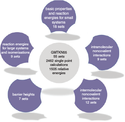
At around the same time as the first MGCDB84 study was published, our group in collaboration with the Grimme group published an update of our GMTKN30 database after having received multiple personal requests by many users and developers that had asked us to continue our contributions to the field. The resulting database is called GMTKN55 and contains 1505 data points separated into 55 benchmark sets that can be divided into the five different categories shown in Fig. 2.[68] Whilst smaller in size than MGCDB84, GMTKN55 has distinct advantages. In particular, we demonstrated that its reference values are of much higher quality than the ones used in GMTKN30 (and therefore also for the benchmark sets that overlap with MGCDB84); in Ref. 68 we demonstrated how that had a significant impact on how to rank DFAs. We also made sure to offer a larger variety of different properties to avoid having a sizeable number of benchmark sets assess the same property repeatedly. Whilst doing so, we also included larger systems, with the largest molecules containing more than 70 atoms. The first GMTKN55 study comprised 217 dispersion-corrected and uncorrected DFAs that broke down into 80 unique dispersion-corrected DFAs for a consistent and detailed analysis.[68] The paper has become a great success and already after a few months Web of Science[73] listed it as a ‘hot paper’, as it was published in the last two years and has reached enough citations to be placed in the top 0.1 % of the academic field of chemistry. This shows the value of such studies to the general chemistry community. In mid 2018, we increased the number of assessed DFAs in two subsequent studies to a total of 325 dispersion-corrected and uncorrected methods, with 115 dispersion-corrected ones being analysed thoroughly.[40,74] We focussed on the four highest rungs on Jacob’s Ladder, as it had already been established that LDA functionals were not viable for molecular chemistry applications.[33] The three papers combined can be regarded as the largest published DFT benchmark study.[40,68,74] We will review our recommendations in one of the following sections. We also note that method developers who cannot use GMTKN55 during the development stage may want to use Gould’s recently published ‘Diet GMTKN55’ before conducting a final assessment on the full GMTKN55.[75]
|
The Importance of London Dispersion
One of the major deficiencies of conventional DFAs is the inability to describe London-dispersion forces, as first shown in the 1990s.[76–79] London dispersion is ubiquitous and stabilises both intra- and intermolecular interactions and the increasing popularity of DFAs and their failure to correctly capture this phenomenon posed a dilemma to users and sparked a tremendous interest to rectify it. Many strategies have emerged and we only briefly summarise the four main categories of dispersion-corrected DFT here; we highly recommend Ref. 80 for a detailed review. The first category represents a very time-efficient strategy, namely to use additive corrections that estimate the missing dispersion energy for a given functional with negligible computational effort, which is added to the electronic energy obtained from a standard DFT calculation. The majority of the missing dispersion energy is accounted for by summing up the dispersion contributions of each atom pair, while three- or many-body interactions can be additionally requested for some types of additive dispersion corrections.[81–83] All additive corrections rely on the molecular geometry as an input and sometimes also electron density or atomic charges to better take into account electronic effects that may alter the dispersion coefficients compared to a bare atom.[24,81–94]. While the idea of using an additive dispersion correction dates back to HF calculations in the 1970s,[95,96] one of the first successful schemes regularly applied by users was Grimme’s DFT-D2 correction,[24] which relies on atom-pair contributions and a small number of empirical atomic C6 dispersion coefficients.† DFT-D2 has had a transforming impact on the broader field of chemistry and in 2016 ‘Chemical & Engineering News’ determined it to be the most-cited chemistry paper published ‘a decade ago’.[97]
DFT-D2 was replaced by DFT-D3 in 2010, which is a far more robust and less empirical method.[81] It does not only use the molecular geometry as an input, but the chemical environment of each individual atom modifies its dispersion coefficients, which introduces some system dependence. DFT-D3 comes in three flavours named DFT-D3(0)[81] (with ‘zero damping’), DFT-D3(BJ)[85] (with ‘Becke-Johnson’ damping[89]), and the less known DFT-D3(CSO)[86] (with ‘C-six-only’ damping).‡ We refer the reader to Refs 80 and 99 for reviews of the details of these technicalities; it shall suffice to say that damping functions are needed to control the overlap region between short-range interactions governed by the underlying DFA and long-range interactions treated by the dispersion correction. Overall, DFT-D3(BJ) should be used, as it is physically more sound,[85] except for those methods that are only compatible with DFT-D3(0), such as most of the Minnesota functionals by the Truhlar group.[56,100] While very recently the new DFT-D4 has been published[87,88] and while it is yet to be seen how it will be adopted by the user community, DFT-D3(0) and DFT-D3(BJ) are currently the most applied dispersion corrections. In fact, DFT-D3(BJ) is our routine choice for larger systems, for which the second category of corrections described in the next paragraph cannot be applied.
The second category contains methods that were designed in an attempt to fix the dispersion problem at its root, namely by including a term that enforces the correct asymptotic behaviour of the dispersion energy.[101–104] That term, also called ‘non-local (NL) kernel’, can in principle be combined with any underlying DFA.[105] Different NL kernels were developed[101–104] and the one suggested by Vydrov and van Voorhis in 2010—the VV10[104] kernel—emerged as the method of choice that is now being used in combination with many functionals. Examples are methods that either end in the suffix ‘V’ (such as B97M-V),[106–108] or ‘NL’ (such as B3LYP-NL).[105] Quantum-chemistry packages, such as ORCA,[109] PSI4[110], QCHEM,[111] or ERKALE[112] offer implementations of the VV10 kernel. While the latter two only allow for its application with a limited number of semi-local DFAs, the first two are more flexible and do not impose any such restrictions. ORCA and PSI4 also offer an additional degree of freedom for the user, namely to choose whether the VV10 kernel is used in the self-consistent-field (SCF) step or whether it is used as an additive (post-SCF) correction to correct the converged energy of the underlying semi-local DFA. While the first strategy may be the preferred one from the purist’s point of view, we conclusively showed with the help of GMTKN55 and other systems that a full-SCF version only has negligible influence on relative energies, electron densities, and orbital gaps.[74] Instead, the post-SCF strategy can reduce the overall computational effort by 50 %.[74]
The third category had its heyday between 2004 and 2014.[113–115] Readers who have carried out calculations with heavier elements may be familiar with the concept of effective core potentials,[116] which are Gaussian-type one-electron potentials that mimic the effect of core electrons including relativistic effects. There have been attempts to use those potentials, which are readily available in every quantum-chemistry code, and refit them against NCI energies. Despite the initial popularity of such an approach, it should be surprising for any theoretician that one-electron potentials were expected to deliver a correct description of an electron-correlation effect, such as London dispersion, for which by definition at least two electrons are needed. Indeed, the first author of this account showed in 2014 that this idea broke down when moving away from inter- to intramolecular interactions and that it created large errors for the latter—both for conformers and thermochemistry.[117] In these days, this approach is not used often, but instead developers have started to make use of similar potentials to solve other problems, such as errors stemming from using small AO basis sets[118,119] or to improve the description of rotational energy profiles.[120]
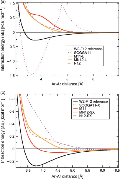
The fourth category is an immensely popular one. It comprises semi-local DFAs that do not contain any terms that actually allow the description of long-range dispersion interactions, but instead they rely on a large number of parameters that were empirically fitted to ‘covalent’ properties and non-covalently bound dimers. The Minnesota classes of functionals,[122,123] with M062X[31] probably being the most famous representative, belong to this category and are the methods of choice for many. Without doubt, some of the Minnesota functionals provide very reliable and accurate results particularly in thermochemistry and the treatment of transition metals.[56,68,122,123] However, when it comes to the treatment of dispersion interactions we have to issue a clear warning to the user: they do not properly capture the physics of dispersion interactions correctly! Back in 2011, Goerigk et al. showed that the early Minnesota functionals severely underestimated interaction energies in the long-range regime[124] and benefitted from additive dispersion corrections even for equilibrium geometries.[56,124] The developers of Minnesota functionals then subsequently changed their stance and stated that they should only capture dispersion effects at van-der-Waals distances where the electron clouds of two non-covalently bound fragments start to overlap.[123] The present first author examined the validity of such a claim in 2015;[100] the main finding is visualised for the argon-dimer dissociation curve and various newer members of the Minnesota family in Fig. 3. The various curves clearly show severe problems in the van-der-Waals and asymptotic regions, sometimes even highly unphysical behaviour with inflection points or spikes. Ref. 100 also showed how the tested functionals could be improved by adding the DFT-D3 correction and it was also the first work to combine a Minnesota functional with the VV10 kernel from the second category (M06L-NL). A year later, Mardirossian and Head-Gordon assessed Minnesota functionals for a large variety of NCI energies and confirmed their inability to properly describe them.[125] Our first GMTKN55 study demonstrated how Minnesota functionals were improved by dispersion corrections throughout all categories of the database, including non-covalently bound systems in their equilibrium geometries.[68] Only three Minnesota methods seemed not to be affected by the DFT-D3 correction, but nevertheless those were by far not competitive enough with other approaches to describe NCIs;[68] these three methods were MN15-L,[126] M06,[31] and MN15.[69] Our recommendation is that users who would like to use Minnesota functionals in their work should not forget about the dispersion problem and should always combine them with a proper dispersion correction in the same way they would for any other conventional functional.
|
The message of the last sentence cannot be emphasised enough: conventional DFAs need to be enhanced with a dispersion correction. In this final paragraph, we briefly summarise why. London dispersion is ubiquitous; however, parts of the chemistry community often underestimate this phenomenon as being small and negligible compared to other interactions, such as electrostatics. Consequently, many DFT users in the 1990s and 2000s ignored the dispersion problem. This is something we can still see nowadays in computational applications that serve to enhance experimental results, even in high-impact journals. It is hoped that more reviewers and editors become aware of this problematic issue. At the same time, it is also comforting to see a welcoming change in the field. In fact, the emergence of dispersion corrections and their subsequent application led to a ‘re-education’ of the user community championed by many groups. Their contributions convincingly showed that the size of dispersion can become comparable with that of other interactions. The list of successful examples is long and would go beyond the scope of this account and we refer to Refs 80 and 99 for more examples. We would only like to emphasise that it is now well-documented that London dispersion goes beyond non-covalently bound dimers. In fact, it influences structural features of molecules and crystals, thermochemical properties, and reaction mechanisms.[40,68,74,127–135] Bulky chemical groups can even serve as ‘dispersion energy donors’[128] to overcome steric repulsion to form novel molecular structures.[127] When paired with a robust DFA, modern dispersion-corrected DFT has unprecedented accuracy and even outperforms some ab initio wave-function methods, as we demonstrated in our largest DFT benchmark study ever published.[40,68,74] This brings us to the next section in which we review our main recommendations for modern dispersion-corrected DFAs.
Our Current Recommendations for Method Users
Herein, we briefly summarise the main findings of our extensive GMTKN55 analysis that comprised 325 variations of dispersion-corrected and -uncorrected DFAs representing 104 unique XC functionals.[40,68,74] In many cases, we applied different dispersion corrections to the same unique functional, but boiled down the final analysis to the most efficient correction: mostly DFT-D3(BJ), sometimes the NL kernel, and only in exceptions the DFT-D3(0) variant. In total, we presented a thorough analysis of 115 of such dispersion-corrected methods. The GMTKN55 papers allow the users to identify the best DFT methods for each of the 55 assessed properties and someone who is interested in a specific property is referred to the supporting information of Ref. 74. However, as outlined earlier, the main motivation behind the database was to identify methods that are robust, accurate, and perform equally well for a range of problems. Such methods should be favoured by users in actual applications, as they should give a reliable result with much higher probability than many of the currently used approaches. In order to provide such a ranking of DFAs, we presented a scheme that allowed us to condense the statistical values for each of the 55 sets to one final number, which we called ‘weighted total mean absolute deviation’ (WTMAD).[68] After having thoroughly assessed 11 different WTMAD schemes, we recommended two, named WTMAD-1 and WTMAD-2.[68] Both schemes delivered the same general trends, which is why we are confident about the validity of our recommendations. According to the WTMAD idea, lower values indicate higher levels of accuracy and robustness. The exact details of how these WTMADs were defined shall not matter for this section and the interested reader is referred to the original paper.[68] WTMADs were presented for each of the categories for GMTKN55 and for the entire set. Herein, we only focus on the latter and summarise our main findings below.
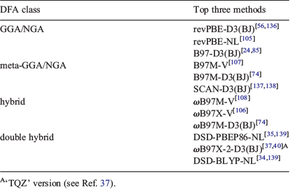
Our first important finding was that dispersion-corrected DFT methods outperformed their uncorrected counterparts and we demonstrated with GMTKN55 that dispersion can influence REs and BHs by 1 kcal mol−1 or significantly more, which is higher than the chemical-accuracy value. Our study also reconfirms the validity of the Jacob’s Ladder scheme with average WTMADs for each individual rung decreasing as one climbs the ladder. As a consequence, dispersion-corrected DHDFs should be the methods of choice and we only recommend hybrids if the first cannot be applied for technical reasons. That being said, not every double hybrid can be safely recommended and we identified a series of DHDFs—often called ‘non-empirical[140]’ double hybrids—that were outperformed by many methods of the fourth rung.[40] In the same way, we also identified hybrids that were outperformed by second- or third-rung functionals.[68] While we strive to update our GMTKN55-based rankings whenever new methods become available, we currently recommend those top three functionals for each of the four highest rungs that are shown in Table 1. LDAs in general cannot be recommended and are therefore not listed. As can be seen, some methods employ the NL kernel; however, if its application is not feasible, one can safely use the faster DFT-D3(BJ) without significant loss in robustness or accuracy. Almost all methods can be used with the latest version of the free program ORCA,[109] which should make the transition to new computational strategies easy for the user. However, if one has to rely on a different program that may not have these methods implemented, we can also recommend the double hybrid B2GPPLYP-D3(BJ)[56,61] and the hybrids M052X-D3(0),[56,122] ωB97X-D3(0),[141] and PW6B95-D3(BJ).[85,142] In the next section, we address better known and more popular methods and their performance for GMTKN55.
|
Popularity versus Accuracy and Reliability
For those who are familiar with DFT applications, the recommendations in the previous section may have come as a surprise, as we did not discuss any of the well-known DFAs, such as B3LYP, PBE0, PBE, or BP86. This section is dedicated to such popular approaches and to the question of whether popularity should be the reason for choosing a method for an application. We would like to add a new perspective to this discussion with the help of an analysis that has not been conducted before. While one can base the popularity of a method on its number of citations (see Supplementary Material for a citation analysis of popular DFAs), we herein would like to focus on the annual ‘DFT poll’ by Swart, Bickelhaupt, and Duran.[143] This poll started in 2010 and separates popular functionals into two divisions—almost akin to soccer leagues—where the top DFAs of the second division will make it into the first division in the following year, while the least popular methods in the first division will be demoted to the second.
In addition, new methods can also be suggested by followers that can then rise through the ranks. While the poll itself has never been published in any of the conventional scientific outlets and while it is hard to gauge the geographical and scientific background of its participants, we still find it an insightful activity. Details of each year’s poll are given on the relevant website and herein we would like to focus solely on those 20 DFAs that made it into the first division of the respective year and compare it to our findings for GMTKN55. Our aim herein is to track and benchmark the performance of the first-division DFAs of each year. This allows us to gain useful insights into how the perception of DFT methods has changed in the user community and if that is reflected by what we as members of the developer community know and recommend based on our thorough benchmark studies.
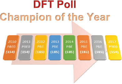
Fig. 4 shows the most popular density functional from each year’s poll and its rank based on the assessments of 216 dispersion-corrected and -uncorrected DFA approaches with GMTKN55.§
|
The results are based on already published data[40,68,74] and three additional DFAs, as outlined in the Supplementary Material. For the context of this analysis ‘dispersion corrected’ refers mostly to the DFT-D3(BJ) correction, unless DFT-D3(0) has been particularly recommended, as well as to the NL correction. A list of the DFT-D3(0) and NL-corrected methods used in this analysis is shown in the Supplementary Material. The ranking of DFAs is based on the WTMAD-2 scheme. Fig. 4 shows that in five out of eight years PBE emerges as the most popular density functional. However, it is only at 185th position for GMTKN55. The next popular DFA approximation, PBE0, appears three times at the top in the DFT polls. PBE0, however, only ranks in 154th position. While it is never at the top, B3LYP has always featured in the first division, and also a citation analysis shows that it is by far one of the most popular functionals in the user community (see Supplementary Material). However, for GMTKN55, it only ranks in 197th position, which is worse than many dispersion-uncorrected GGAs! We also note that none of the popular functionals were suggested to be used with a dispersion correction. In fact, only three of the top-20 methods were chosen with a dispersion correction in the 2017 poll, usually the outdated DFT-D2. However, even if we apply the DFT-D3 correction to PBE and PBE0, the resulting dispersion-corrected approaches still show mediocre performance and they rank in 140th and 77th position for GMTKN55, respectively. B3LYP-D3 appears in 72nd position.
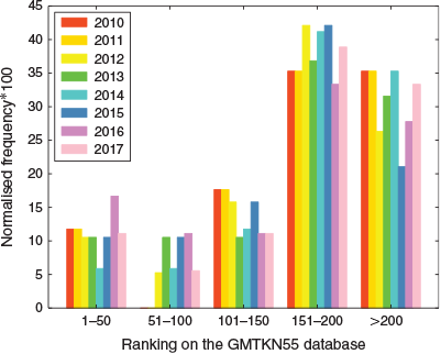
After having focussed on the most popular approaches at the top of the first division, we now proceed with a comprehensive look at all first-division DFAs in each year. For that we calculated the rankings of those DFAs for the GMTKN55 database, which required some additional calculations, as some functionals had not been assessed before (see Supplementary Material for more details). For each year, all functionals were ranked based on their WTMAD-2 values and divided into bins of 50 ranking positions for the GMTKN55 database. Each functional belonging to a particular bin gave a count of one to the frequency. Note that some first-division functionals were excluded from our analysis, as they either had been designed for specific properties or they were technically not feasible; therefore, the overall count to the first-division DFAs used in our analysis for some years was not always 20. To accommodate this, we normalised the frequencies in each bin by dividing them by the respective number of tested functionals for a given year. The resulting plot shown in Fig. 5 allows us to gauge if and how preferences of the DFT user community have changed and whether the comprehensive benchmark studies have made an impact on those. Unfortunately, we do not see that the poll started to favour more accurate approaches. If it had done so, we would see higher bars in the top-50 bin for the most recent years. It is striking that even in the 2017 poll one third of the first-division methods belong to the 16 worst DFA approaches for GMTKN55! We also note in passing that DHDFs, even though they have been shown to be the most robust DFT methods have not had a significant influence on the first division over the years.
|
In the Supplementary Material, we demonstrate a third analysis of the DFT-poll data, which is more specialised and may only be relevant to some readers. Also that analysis shows the same picture as before, namely that we cannot see any significant improvement over the years despite the emergence of better functionals and thorough benchmark studies. Our analysis clearly shows the communication gap between the developers and users mentioned in the introduction. It also shows the need to continuously engage with users, as is our intention with this account. We hope that the continuing reiteration of our findings, including the new angle from which we have viewed this topic in this section, will inspire long-needed rethinking in the user community.
Structural Properties
The majority of this account has dealt with single-point energy calculations and the analysis of energetic properties. However, most quantum-chemical studies commence with an optimisation of structural parameters. Similarly to the calculation of energetic properties, this field is governed by approaches that are chosen due to popularity rather than an informed decision. First of all, we have to state that Jacob’s Ladder is also reproducible for geometries; however, the differences between the rungs are smaller, such that optimisations with DHDFs are usually not required.[144,145] Depending on system size, hybrid or (meta-)GGA functionals are sufficient in our experience. Many users prefer the B3LYP hybrid and the BP86 GGA, often paired with relatively small AO basis sets, in particular 6-31G*.[146] This is very similar to many energy calculations in the computational organic chemistry field, where B3LYP/6-31G* seems to be the preferred standard.
In this section, we briefly review our previous works on the optimisation of polypeptides, but the general messages can be transferred to any system of similar size or larger, in particular for organic molecules and transition-metal complexes. When we set out to work on polypeptide optimisations, B3LYP and BP86 seemed to be the methods of choice in the field, which came as a surprise. The importance of London dispersion to the structural stability of biomolecules is well-established,[147] and yet DFT methods were chosen that did not treat any such interactions, which is a striking contradiction. In fact, similarly to what we outlined for energetics earlier, it is also well known how geometries become more accurate when dispersion corrections are applied (we will see a visual example for this very shortly).[80,85,99,127,145,148] The second problem is the quality of the often-applied small AO basis sets. The more AOs we use, the more reliable the LCAO approximation to the molecular orbitals is. However, using large basis sets requires more computational resources. Consequently, the user has to strike a compromise between reliability and computational effort. However, one also has to consider the risks that stem from having an incomplete basis. One portion of this incompleteness error is often forgotten by the user community. It is called the ‘basis-set superposition error’ (BSSE) and manifests itself in an artificial overestimation of NCIs.[18] Herein, we would like to remind that this problem is not unique to non-covalently bound dimers, but also to intramolecular interactions. As such, any overestimated NCI should distort the resulting geometry of a molecule, as we will see below.
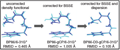
The efficient treatment of both the inter- and intramolecular BSSEs became possible with Kruse and Grimme’s additive ‘geometrical counterpoise’ (gCP) correction,[149] and with the conceptually related ‘DFT-C’ method by Head-Gordon and co-workers.[150] For energy calculations, Kruse, Goerigk, and Grimme showed how the infamous B3LYP/6-31G* level of theory can be turned into something more robust and reliable when combined with DFT-D3 and gCP without compromising its beneficial computational cost.[14] In Fig. 6, we see that the same is also true for geometries, as shown for a folded conformer of phenylalanyl-glycyl-glycine (FGG).[134] The light blue structure is based on the popular BP86/6-31G* level of theory and it is compared with an ab initio structure that provides sufficient accuracy for the main message that this figure conveys. For this conformer, one would expect significant NCIs between both ends. If BSSE plays a role, it should lead for the two ends to be too close to one another. Indeed, one sees how they move away from one another after addition of the gCP correction (middle of Fig. 6). When DFT-D3(BJ) is added, one obtains nearly perfect agreement with the reference structure (Fig. 6). This figure demonstrates one of the possible reasons for the popularity of BP86/6-31G* or B3LYP/6-31G*. While dispersion is not described, BSSE mimics some attractive effects, therefore creating a seemingly better structure, as can be seen by the relatively low root-mean square deviation in Fig. 6. This effect is clearly due to error compensation, something that one should avoid relying on due to its unpredictability. By adding both corrections, one ensures the right result is obtained for the right reason. We later verified these findings for the geometry optimisation of a protein fragment in its crystal environment compared against a highly accurate experimental structure.[135]
|
As BSSE is only one problem related to incomplete basis sets, we recommend to always use a basis set of at least triple-ζ quality. If that is not possible, applying a BSSE correction is required. To avoid any remaining basis-set-incompleteness errors, we specifically recommend the relatively new DFT methods by the Grimme group called PBEh-3c[151] and B97-3c,[152] which take into account dispersion and provide accurate geometries for large systems whilst keeping any basis-set errors minimal.
Concluding Remarks
This account cannot replace detailed review articles or textbooks, but we do hope that it provides readers with guidelines that informs them on which computational strategies to best follow. A particular emphasis was laid on the fact that popularity should never justify a chosen computational strategy. Instead, we can rely on the results of thorough benchmarking studies that allow us to pick our methods based on evidence. As such, we hope to have also convinced the reader that benchmark studies themselves play an important role, as they can offer novel insights into the general chemistry community, such as that demonstrated by the success of benchmarking London-dispersion corrections, which revealed how crucial London dispersion is for structures and reactivity alike. To the general user and anyone new to the field, the zoo of DFT methods can be intimidating and we hope we have shed some light on this complex field. The most important take-home messages of this account can be summarised as follows:
-
London dispersion has to be taken into account in general computational (thermo-)chemistry.
-
Dispersion-corrected, semi-empirical double hybrids are the most accurate DFT methods for ground-state thermochemistry.
-
Various dispersion corrections exist and they differ in accuracy and applicability. While we do not want to discourage users from applying Minnesota functionals, we caution them when it comes to applying them without any dispersion corrections. In fact, dispersion-corrected M052X-D3(0) turned out to be a good approach for general main-group thermochemistry, kinetics and non-covalent interactions.[68]
-
London dispersion and basis-set effects have to be considered in structure optimisations.
We hope that our take on the topics discussed in this account are helpful to some. We would like to encourage further reading of the herein cited articles if more detail is required. Ultimately, we hope we can make a valuable contribution towards future computational endeavours.
Supplementary Material
More details on the analysis of the first-division DFAs for each year of the DFT poll, a citation analysis of the first-division DFAs in the DFT polls and statistical data for GMTKN55 for DFAs that were newly tested in this work are available on the Journal’s website.
Conflicts of Interest
The authors declare no conflicts of interest.
Acknowledgements
We would like to thank Profs Marcel Swart, Matthias Bickelhaupt, and Miquel Duran for conducting the annual DFT poll and making the results freely accessible to the public. LG acknowledges the 2017 RACI Physical Chemistry Division Lectureship awarded by the Royal Australian Chemical Institute. LG is also grateful for generous resource allocations from Melbourne Bioinformatics (Project RA0005) and the National Computational Infrastructure (NCI) National Facility within the National Computational Merit Allocation Scheme (Project fk5) over the past years. NM is the recipient of a ‘Melbourne International Engagement Award’ (MIEA) offered through the Melbourne India Postgraduate Program and a ‘Melbourne Research Scholarship’.
References
[1] W. Kohn, L. J. Sham, Phys. Rev. 1965, 140, A1133.| Crossref | GoogleScholarGoogle Scholar |
[2] D. C. Langreth, J. P. Perdew, Phys. Rev. B Condens. Matter 1980, 21, 5469.
| Crossref | GoogleScholarGoogle Scholar |
[3] D. C. Langreth, M. J. Mehl, Phys. Rev. B Condens. Matter 1983, 28, 1809.
| Crossref | GoogleScholarGoogle Scholar |
[4] J. P. Perdew, Phys. Rev. B Condens. Matter 1986, 33, 8822.
| Crossref | GoogleScholarGoogle Scholar | 9938299PubMed |
[5] J. P. Perdew, Phys. Rev. B Condens. Matter 1986, 34, 7406.
| Crossref | GoogleScholarGoogle Scholar | 9949100PubMed |
[6] A. D. Becke, J. Chem. Phys. 1986, 84, 4524.
| Crossref | GoogleScholarGoogle Scholar |
[7] A. D. Becke, Phys. Rev. A 1988, 38, 3098.
| Crossref | GoogleScholarGoogle Scholar |
[8] C. Lee, W. Yang, R. G. Parr, Phys. Rev. B Condens. Matter 1988, 37, 785.
| Crossref | GoogleScholarGoogle Scholar | 9944570PubMed |
[9] B. Miehlich, A. Savin, H. Stoll, H. Preuss, Chem. Phys. Lett. 1989, 157, 200.
| Crossref | GoogleScholarGoogle Scholar |
[10] J. P. Perdew, in Proceedings of the 21st Annual International Symposium on the Electronic Structure of Solids (Eds P. Ziesche, H. Eschrig) 1991, p. 11 (Akademie Verlag: Berlin).
[11] J. P. Perdew, K. Burke, M. Ernzerhof, Phys. Rev. Lett. 1996, 77, 3865.
| Crossref | GoogleScholarGoogle Scholar | 10062328PubMed |
[12] A. D. Becke, J. Chem. Phys. 1993, 98, 1372.
| Crossref | GoogleScholarGoogle Scholar |
[13] A. D. Becke, J. Chem. Phys. 1993, 98, 5648.
| Crossref | GoogleScholarGoogle Scholar |
[14] H. Kruse, L. Goerigk, S. J. Grimme, J. Org. Chem. 2012, 77, 10824.
| Crossref | GoogleScholarGoogle Scholar | 23153035PubMed |
[15] P. Hohenberg, W. Kohn, Phys. Rev. B 1964, 136, 864.
| Crossref | GoogleScholarGoogle Scholar |
[16] J. P. Perdew, K. Schmidt, AIP Conf. Proc. 2001, 577, 1.
| Crossref | GoogleScholarGoogle Scholar |
[17] A. Szabo, N. S. Ostlund, Modern Quantum Chemistry: Introduction to Advanced Electronic Structure Theory 1989 (McGraw-Hill: New York, NY).
[18] See pp. 254–255 in: F. Jensen Introduction to Computational Chemistry, 3rd edn 2017 (Wiley: Chichester).
[19] W. Koch, M. C. Holthausen, A Chemist’s Guide to Density Functional Theory, 2nd edn 2001 (Wiley-VCH: New York, NY).
[20] P.-F. Loos, P. M. W. Gill, Wiley Interdiscip. Rev. Comput. Mol. Sci. 2016, 6, 410.
| Crossref | GoogleScholarGoogle Scholar |
[21] J. C. Slater, Phys. Rev. 1951, 81, 385.
| Crossref | GoogleScholarGoogle Scholar |
[22] S. J. Vosko, L. Wilk, M. Nusair, Can. J. Phys. 1980, 58, 1200.
| Crossref | GoogleScholarGoogle Scholar |
[23] J. P. Perdew, Y. Wang, Phys. Rev. B Condens. Matter 1992, 45, 13244.
| Crossref | GoogleScholarGoogle Scholar | 10001404PubMed |
[24] S. Grimme, J. Comput. Chem. 2006, 27, 1787.
| Crossref | GoogleScholarGoogle Scholar | 16955487PubMed |
[25] R. Peverati, D. G. Truhlar, J. Chem. Theory Comput. 2012, 8, 2310.
| Crossref | GoogleScholarGoogle Scholar | 26588964PubMed |
[26] J. Tao, J. P. Perdew, V. N. Staroverov, G. E. Scuseria, Phys. Rev. Lett. 2003, 91, 146401.
| Crossref | GoogleScholarGoogle Scholar | 14611541PubMed |
[27] Y. Zhao, D. G. Truhlar, J. Chem. Phys. 2006, 125, 194101.
| Crossref | GoogleScholarGoogle Scholar | 17129083PubMed |
[28] M. Ernzerhof, G. E. Scuseria, J. Chem. Phys. 1999, 110, 5029.
| Crossref | GoogleScholarGoogle Scholar |
[29] C. Adamo, V. Barone, J. Chem. Phys. 1999, 110, 6158.
| Crossref | GoogleScholarGoogle Scholar |
[30] P. J. Stephens, F. J. Devlin, C. F. Chabalowski, M. J. Frisch, J. Phys. Chem. 1994, 98, 11623.
| Crossref | GoogleScholarGoogle Scholar |
[31] Y. Zhao, D. G. Truhlar, Theor. Chem. Acc. 2008, 120, 215.
| Crossref | GoogleScholarGoogle Scholar |
[32] S. Grimme, J. Chem. Phys. 2006, 124, 034108.
| Crossref | GoogleScholarGoogle Scholar | 16438568PubMed |
[33] L. Goerigk, S. Grimme, J. Chem. Theory Comput. 2011, 7, 291.
| Crossref | GoogleScholarGoogle Scholar | 26596152PubMed |
[34] S. Kozuch, D. Gruzman, J. M. L. Martin, J. Phys. Chem. C 2010, 114, 20801.
| Crossref | GoogleScholarGoogle Scholar |
[35] S. Kozuch, J. M. L. Martin, Phys. Chem. Chem. Phys. 2011, 13, 20104.
| Crossref | GoogleScholarGoogle Scholar | 21993810PubMed |
[36] S. Kozuch, J. M. L. Martin, J. Comput. Chem. 2013, 34, 2327.
| Crossref | GoogleScholarGoogle Scholar | 23983204PubMed |
[37] J.-D. Chai, M. Head-Gordon, J. Chem. Phys. 2009, 131, 174105.
| Crossref | GoogleScholarGoogle Scholar | 19894996PubMed |
[38] N. Mardirossian, M. Head-Gordon, J. Chem. Phys. 2018, 148, 241736.
| Crossref | GoogleScholarGoogle Scholar | 29960332PubMed |
[39] L. Goerigk, S. Grimme, Wiley Interdiscip. Rev. Comput. Mol. Sci. 2014, 4, 576.
| Crossref | GoogleScholarGoogle Scholar |
[40] N. Mehta, M. Casanova-Páez, L. Goerigk, Phys. Chem. Chem. Phys. 2018, 20, 23175.
| Crossref | GoogleScholarGoogle Scholar | 30062343PubMed |
[41] R. M. Irelan, T. M. Henderson, G. E. Scuseria, J. Chem. Phys. 2011, 135, 094105.
| Crossref | GoogleScholarGoogle Scholar | 21913751PubMed |
[42] H. Eshuis, F. Furche, J. Phys. Chem. Lett. 2011, 2, 983.
| Crossref | GoogleScholarGoogle Scholar |
[43] A. J. Garza, I. W. Bulik, A. G. S. Alencar, J. Sun, J. P. Perdew, G. E. Scuseria, Mol. Phys. 2016, 114, 997.
| Crossref | GoogleScholarGoogle Scholar |
[44] S. Grimme, M. Steinmetz, Phys. Chem. Chem. Phys. 2016, 18, 20926.
| Crossref | GoogleScholarGoogle Scholar | 26695184PubMed |
[45] P. D. Mezei, G. I. Csonka, A. Ruzsinszky, M. Kállay, J. Chem. Theory Comput. 2015, 11, 4615.
| Crossref | GoogleScholarGoogle Scholar | 26574252PubMed |
[46] P. D. Mezei, G. I. Csonka, A. Ruzsinszky, M. Kállay, J. Chem. Theory Comput. 2017, 13, 796.
| Crossref | GoogleScholarGoogle Scholar | 28052197PubMed |
[47] J. Almlöf, Chem. Phys. Lett. 1991, 181, 319.
| Crossref | GoogleScholarGoogle Scholar |
[48] Y. S. Jung, R. C. Lochan, A. D. Dutoi, M. Head-Gordon, J. Chem. Phys. 2004, 121, 9793.
| Crossref | GoogleScholarGoogle Scholar |
[49] O. Vahtras, J. Almlöf, M. W. Feyereisen, Chem. Phys. Lett. 1993, 213, 514.
| Crossref | GoogleScholarGoogle Scholar |
[50] K. Raghavachari, A. Saha, Chem. Rev. 2015, 115, 5643.
| Crossref | GoogleScholarGoogle Scholar | 25849163PubMed |
[51] A. Karton, Wiley Interdiscip. Rev. Comput. Mol. Sci. 2016, 6, 292.
| Crossref | GoogleScholarGoogle Scholar |
[52] L. A. Curtiss, K. Raghavachari, G. W. Trucks, J. A. Pople, J. Chem. Phys. 1991, 94, 7221.
| Crossref | GoogleScholarGoogle Scholar |
[53] L. A. Curtiss, K. Raghavachari, P. C. Redfern, J. A. Pople, J. Chem. Phys. 1997, 106, 1063.
| Crossref | GoogleScholarGoogle Scholar |
[54] L. A. Curtiss, K. Raghavachari, P. C. Redfern, V. Rassolov, J. A. Pople, J. Chem. Phys. 1998, 109, 7764.
| Crossref | GoogleScholarGoogle Scholar |
[55] L. A. Curtiss, P. C. Redfern, K. Raghavachari, J. Chem. Phys. 2005, 123, 124107.
| Crossref | GoogleScholarGoogle Scholar | 16392475PubMed |
[56] L. Goerigk, S. Grimme, Phys. Chem. Chem. Phys. 2011, 13, 6670.
| Crossref | GoogleScholarGoogle Scholar | 21384027PubMed |
[57] Y. Zhao, B. J. Lynch, D. G. Truhlar, Phys. Chem. Chem. Phys. 2005, 7, 43.
| Crossref | GoogleScholarGoogle Scholar |
[58] Y. Zhao, N. González-García, D. G. Truhlar, J. Phys. Chem. A 2005, 109, 2012.
| Crossref | GoogleScholarGoogle Scholar | 16833536PubMed |
[59] P. Jurečka, J. Sponer, J. Cerny, P. Hobza, Phys. Chem. Chem. Phys. 2006, 8, 1985.
| Crossref | GoogleScholarGoogle Scholar | 16633685PubMed |
[60] J. Rezáč, K. E. Riley, P. Hobza, J. Chem. Theory Comput. 2011, 7, 2427.
| Crossref | GoogleScholarGoogle Scholar | 21836824PubMed |
[61] A. Karton, A. Tarnopolsky, J. F. Lamere, G. C. Schatz, J. M. L. Martin, J. Phys. Chem. A 2008, 112, 12868.
| Crossref | GoogleScholarGoogle Scholar | 18714947PubMed |
[62] D. Gruzman, A. Karton, J. M. L. Martin, J. Phys. Chem. A 2009, 113, 11974.
| Crossref | GoogleScholarGoogle Scholar | 19795892PubMed |
[63] A. Karton, S. Daon, J. M. L. Martin, B. Ruscic, Chem. Phys. Lett. 2011, 510, 165.
| Crossref | GoogleScholarGoogle Scholar |
[64] S. Grimme, M. Steinmetz, M. Korth, J. Org. Chem. 2007, 72, 2118.
| Crossref | GoogleScholarGoogle Scholar | 17286442PubMed |
[65] M. Korth, S. Grimme, J. Chem. Theory Comput. 2009, 5, 993.
| Crossref | GoogleScholarGoogle Scholar | 26609608PubMed |
[66] K. Raghavachari, G. W. Trucks, J. A. Pople, M. Head-Gordon, Chem. Phys. Lett. 1989, 157, 479.
| Crossref | GoogleScholarGoogle Scholar |
[67] D. Beckett, T. J. El-Baba, D. E. Clemmer, K. Raghavachari, J. Chem. Theory Comput. 2018, 14, 5406.
| Crossref | GoogleScholarGoogle Scholar | 30192543PubMed |
[68] L. Goerigk, A. Hansen, C. Bauer, S. Ehrlich, A. Najibi, S. Grimme, Phys. Chem. Chem. Phys. 2017, 19, 32184.
| Crossref | GoogleScholarGoogle Scholar | 29110012PubMed |
[69] H. S. Yu, X. He, S. L. Li, D. G. Truhlar, Chem. Sci. 2016, 7, 5032.
| Crossref | GoogleScholarGoogle Scholar | 30155154PubMed |
[70] L. Goerigk, S. Grimme, J. Chem. Theory Comput. 2010, 6, 107.
| Crossref | GoogleScholarGoogle Scholar | 26614324PubMed |
[71] N. Mardirossian, M. Head-Gordon, Mol. Phys. 2017, 115, 2315.
| Crossref | GoogleScholarGoogle Scholar |
[72] B. Chan, J. Chem. Theory Comput. 2018, 14, 4254.
| Crossref | GoogleScholarGoogle Scholar | 30004698PubMed |
[73] Web of Science Core Collection, see http://www.webofscience.com
[74] A. Najibi, L. Goerigk, J. Chem. Theory Comput. 2018, 14, 5725.
| Crossref | GoogleScholarGoogle Scholar | 30299953PubMed |
[75] T. Gould, Phys. Chem. Chem. Phys. 2018, 20, 27735.
| Crossref | GoogleScholarGoogle Scholar | 30387792PubMed |
[76] S. Kristyán, P. Pulay, Chem. Phys. Lett. 1994, 229, 175.
| Crossref | GoogleScholarGoogle Scholar |
[77] J. Pérez-Jordá, A. D. Becke, Chem. Phys. Lett. 1995, 233, 134.
| Crossref | GoogleScholarGoogle Scholar |
[78] P. Hobza, J. Sponer, T. Reschel, J. Comput. Chem. 1995, 16, 1315.
| Crossref | GoogleScholarGoogle Scholar |
[79] J. Sponer, J. Leszczynski, P. Hobza, J. Comput. Chem. 1996, 17, 841.
| Crossref | GoogleScholarGoogle Scholar |
[80] S. Grimme, A. Hansen, J. G. Brandenburg, C. Bannwarth, Chem. Rev. 2016, 116, 5105.
| Crossref | GoogleScholarGoogle Scholar | 27077966PubMed |
[81] S. Grimme, J. Antony, S. Ehrlich, H. Krieg, J. Chem. Phys. 2010, 132, 154104.
| Crossref | GoogleScholarGoogle Scholar | 20423165PubMed |
[82] A. Tkatchenko, R. A. DiStasio, R. Car, M. Scheffler, Phys. Rev. Lett. 2012, 108, 236402.
| Crossref | GoogleScholarGoogle Scholar | 23003978PubMed |
[83] A. Ambrosetti, A. M. Reilly, R. A. DiStasio, A. Tkatchenko, J. Chem. Phys. 2014, 140, 18A508.
| Crossref | GoogleScholarGoogle Scholar | 24832316PubMed |
[84] S. Grimme, J. Comput. Chem. 2004, 25, 1463.
| Crossref | GoogleScholarGoogle Scholar | 15224390PubMed |
[85] S. Grimme, S. Ehrlich, L. Goerigk, J. Comput. Chem. 2011, 32, 1456.
| Crossref | GoogleScholarGoogle Scholar | 21370243PubMed |
[86] H. Schröder, A. Creon, T. Schwabe, J. Chem. Theory Comput. 2015, 11, 3163.
| Crossref | GoogleScholarGoogle Scholar | 26575753PubMed |
[87] E. Caldeweyher, C. Bannwarth, S. Grimme, J. Chem. Phys. 2017, 147, 034112.
| Crossref | GoogleScholarGoogle Scholar | 28734285PubMed |
[88] E. Caldeweyher, S. Ehlert, A. Hansen, H. Neugebauer, S. Spicher, C. Bannwarth, S. Grimme, ChemRxiv 2018,
| Crossref | GoogleScholarGoogle Scholar |
[89] A. D. Becke, E. R. Johnson, J. Chem. Phys. 2005, 123, 154101.
| Crossref | GoogleScholarGoogle Scholar | 16252936PubMed |
[90] E. R. Johnson, A. D. Becke, J. Chem. Phys. 2006, 124, 174104.
| Crossref | GoogleScholarGoogle Scholar | 16689564PubMed |
[91] A. D. Becke, E. R. Johnson, J. Chem. Phys. 2007, 127, 154108.
| Crossref | GoogleScholarGoogle Scholar | 17949133PubMed |
[92] A. Tkatchenko, M. Scheffler, Phys. Rev. Lett. 2009, 102, 073005.
| Crossref | GoogleScholarGoogle Scholar | 19257665PubMed |
[93] S. N. Steinmann, C. Corminboeuf, J. Chem. Theory Comput. 2010, 6, 1990.
| Crossref | GoogleScholarGoogle Scholar | 26615928PubMed |
[94] S. N. Steinmann, C. Corminboeuf, J. Chem. Phys. 2011, 134, 044117.
| Crossref | GoogleScholarGoogle Scholar | 21280697PubMed |
[95] J. Hepburn, G. Scoles, R. Penco, Chem. Phys. Lett. 1975, 36, 451.
| Crossref | GoogleScholarGoogle Scholar |
[96] R. Ahlrichs, R. Penco, G. Scoles, Chem. Phys. 1977, 19, 119.
| Crossref | GoogleScholarGoogle Scholar |
[97] C&En Year in Review 2016, see: http://yearinreview.cenmag.org/lookback-at-2006/post-1576.
[98] M. J. Frisch, G. W. Trucks, H. B. Schlegel, G. E. Scuseria, M. A. Robb, J. R. Cheeseman, G. Scalmani, V. Barone, B. Mennucci, G. A. Petersson, et al., Gaussian 16 2016 (Gaussian, Inc.: Wallingford, CT).
[99] L. Goerigk, in Non-Covalent Interactions in Quantum Chemistry and Physics (Eds A. Otero de la Roza, G. A. DiLabio) 2017, pp 195–219 (Elsevier: Amsterdam).
[100] L. Goerigk, J. Phys. Chem. Lett. 2015, 6, 3891.
| Crossref | GoogleScholarGoogle Scholar | 26722889PubMed |
[101] M. Dion, H. Rydberg, E. Schröder, D. C. Langreth, B. I. Lundqvist, Phys. Rev. Lett. 2004, 92, 246401.
| Crossref | GoogleScholarGoogle Scholar | 15245113PubMed |
[102] O. A. Vydrov, T. Van Voorhis, Phys. Rev. Lett. 2009, 103, 063004.
| Crossref | GoogleScholarGoogle Scholar | 19792562PubMed |
[103] K. Lee, E. D. Murray, L. Kong, B. I. Lundqvist, D. C. Langreth, Phys. Rev. B Condens. Matter Mater. Phys. 2010, 82, 081101.
| Crossref | GoogleScholarGoogle Scholar |
[104] O. A. Vydrov, T. J. Van Voorhis, Chem. Phys. 2010, 133, 244103.
| Crossref | GoogleScholarGoogle Scholar |
[105] W. Hujo, S. Grimme, J. Chem. Theory Comput. 2011, 7, 3866.
| Crossref | GoogleScholarGoogle Scholar | 26598333PubMed |
[106] N. Mardirossian, M. Head-Gordon, Phys. Chem. Chem. Phys. 2014, 16, 9904.
| Crossref | GoogleScholarGoogle Scholar | 24430168PubMed |
[107] N. Mardirossian, M. Head-Gordon, J. Chem. Phys. 2015, 142, 074111.
| Crossref | GoogleScholarGoogle Scholar | 25702006PubMed |
[108] N. Mardirossian, M. Head-Gordon, J. Chem. Phys. 2016, 144, 214110.
| Crossref | GoogleScholarGoogle Scholar | 27276948PubMed |
[109] F. Neese, Wiley Interdiscip. Rev. Comput. Mol. Sci. 2012, 2, 73.
| Crossref | GoogleScholarGoogle Scholar |
[110] J. M. Turney, A. C. Simmonett, R. M. Parrish, E. G. Hohenstein, F. A. Evangelista, J. T. Fermann, B. J. Mintz, L. A. Burns, J. J. Wilke, M. L. Abrams, N. J. Russ, M. L. Leininger, C. L. Janssen, E. T. Seidl, W. D. Allen, H. F. Schaefer, R. A. King, E. F. Valeev, C. D. Sherrill, T. D. Crawford, Wiley Interdiscip. Rev. Comput. Mol. Sci. 2012, 2, 556.
| Crossref | GoogleScholarGoogle Scholar |
[111] Y. Shao, Z. Gan, E. Epifanovsky, A. T. Gilbert, M. Wormit, J. Kussmann, A. W. Lange, A. Behn, J. Deng, X. Feng, et al. Mol. Phys. 2015, 113, 184.
| Crossref | GoogleScholarGoogle Scholar |
[112] J. Lehtola, M. Hakala, A. Sakko, K. Hämäläinen, J. Comput. Chem. 2012, 33, 1572.
| Crossref | GoogleScholarGoogle Scholar | 22528614PubMed |
[113] O. A. von Lilienfeld, I. Tavernelli, U. Rothlisberger, D. Sebastiani, Phys. Rev. Lett. 2004, 93, 153004.
| Crossref | GoogleScholarGoogle Scholar | 15524874PubMed |
[114] G. A. DiLabio, Chem. Phys. Lett. 2008, 455, 348.
| Crossref | GoogleScholarGoogle Scholar |
[115] E. Torres, G. A. DiLabio, J. Phys. Chem. Lett. 2012, 3, 1738.
| Crossref | GoogleScholarGoogle Scholar | 26291852PubMed |
[116] T. Starkloff, J. D. Joannopoulos, Phys. Rev. B 1977, 16, 5212.
| Crossref | GoogleScholarGoogle Scholar |
[117] L. Goerigk, J. Chem. Theory Comput. 2014, 10, 968.
| Crossref | GoogleScholarGoogle Scholar | 26580176PubMed |
[118] A. Otero-de-la-Roza, G. A. DiLabio, J. Chem. Theory Comput. 2017, 13, 3505.
| Crossref | GoogleScholarGoogle Scholar | 28636358PubMed |
[119] V. K. Prasad, A. Otero-de-la Roza, G. A. DiLabio, J. Chem. Theory Comput. 2018, 14, 726.
| Crossref | GoogleScholarGoogle Scholar | 29262249PubMed |
[120] D. N. Tahchieva, D. Bakowies, R. Ramakrishnan, O. A. von Lilienfeld, J. Chem. Theory Comput. 2018, 14, 4806.
| Crossref | GoogleScholarGoogle Scholar | 30011363PubMed |
[121] A. Karton, J. M. L. Martin, J. Chem. Phys. 2012, 136, 124114.
| Crossref | GoogleScholarGoogle Scholar | 22462842PubMed |
[122] Y. Zhao, N. E. Schultz, D. G. Truhlar, J. Chem. Theory Comput. 2006, 2, 364.
| Crossref | GoogleScholarGoogle Scholar | 26626525PubMed |
[123] R. Peverati, D. G. Truhlar, Philos. Trans. R. Soc. A 2014, 372, 20120476.
| Crossref | GoogleScholarGoogle Scholar |
[124] L. Goerigk, H. Kruse, S. Grimme, ChemPhysChem 2011, 12, 3421.
| Crossref | GoogleScholarGoogle Scholar | 22113958PubMed |
[125] N. Mardirossian, M. Head-Gordon, J. Chem. Theory Comput. 2016, 12, 4303.
| Crossref | GoogleScholarGoogle Scholar | 27537680PubMed |
[126] H. S. Yu, X. He, D. G. Truhlar, J. Chem. Theory Comput. 2016, 12, 1280.
| Crossref | GoogleScholarGoogle Scholar | 26722866PubMed |
[127] S. Grimme, P. R. Schreiner, Angew. Chem. Int. Ed. 2011, 50, 12639.
| Crossref | GoogleScholarGoogle Scholar |
[128] S. Grimme, R. Huenerbein, S. Ehrlich, ChemPhysChem 2011, 12, 1258.
| Crossref | GoogleScholarGoogle Scholar | 21445954PubMed |
[129] J. P. Wagner, P. R. Schreiner, Angew. Chem. Int. Ed. 2015, 54, 12274.
| Crossref | GoogleScholarGoogle Scholar |
[130] S. Rösel, H. Quanz, C. Logemann, J. Becker, E. Mossou, L. Cañadillas-Delgado, E. Caldeweyher, S. Grimme, P. R. Schreiner, J. Am. Chem. Soc. 2017, 139, 7428.
| Crossref | GoogleScholarGoogle Scholar | 28502175PubMed |
[131] J. R. Reimers, D. Panduwinata, J. Visser, Y. Chin, C. Tang, L. Goerigk, M. J. Ford, M. Sintic, T.-J. Sum, M. J. J. Coenen, B. L. M. Hendriksen, J. A. A. W. Elemans, N. S. Hush, M. J. Crossley, Proc. Natl. Acad. Sci. USA 2015, 112, E6101.
| Crossref | GoogleScholarGoogle Scholar | 26512115PubMed |
[132] A. Karton, L. Goerigk, J. Comput. Chem. 2015, 36, 622.
| Crossref | GoogleScholarGoogle Scholar | 25649643PubMed |
[133] L. Goerigk, R. Sharma, Can. J. Chem. 2016, 94, 1133.
| Crossref | GoogleScholarGoogle Scholar |
[134] L. Goerigk, J. R. Reimers, J. Chem. Theory Comput. 2013, 9, 3240.
| Crossref | GoogleScholarGoogle Scholar | 26583999PubMed |
[135] L. Goerigk, C. A. Collyer, J. R. Reimers, J. Phys. Chem. B 2014, 118, 14612.
| Crossref | GoogleScholarGoogle Scholar | 25410613PubMed |
[136] Y. Zhang, W. Yang, Phys. Rev. Lett. 1998, 80, 890.
| Crossref | GoogleScholarGoogle Scholar |
[137] J. Sun, A. Ruzsinszky, J. P. Perdew, Phys. Rev. Lett. 2015, 115, 036402.
| Crossref | GoogleScholarGoogle Scholar | 26230809PubMed |
[138] J. G. Brandenburg, J. E. Bates, J. Sun, J. P. Perdew, Phys. Rev. B 2016, 94, 115144.
| Crossref | GoogleScholarGoogle Scholar |
[139] F. Yu, J. Chem. Theory Comput. 2014, 10, 4400.
| Crossref | GoogleScholarGoogle Scholar | 26588137PubMed |
[140] E. Brémond, I. Ciofini, J. C. Sancho-Garcia, C. Adamo, Acc. Chem. Res. 2016, 49, 1503.
| Crossref | GoogleScholarGoogle Scholar | 27494122PubMed |
[141] Y.-S. Lin, G.-D. Li, S.-P. Mao, J.-D. Chai, J. Chem. Theory Comput. 2013, 9, 263.
| Crossref | GoogleScholarGoogle Scholar | 26589028PubMed |
[142] Y. Zhao, D. G. Truhlar, J. Phys. Chem. A 2005, 109, 5656.
| Crossref | GoogleScholarGoogle Scholar | 16833898PubMed |
[143] http://www.marcelswart.eu/dft-poll/.
[144] F. Neese, T. Schwabe, S. J. Grimme, Chem. Phys. 2007, 126, 124115.
| Crossref | GoogleScholarGoogle Scholar |
[145] P. Kraus, I. Frank, J. Phys. Chem. A 2018, 122, 4894.
| Crossref | GoogleScholarGoogle Scholar | 29750513PubMed |
[146] W. J. Hehre, R. Ditchfield, J. A. Pople, J. Chem. Phys. 1972, 56, 2257.
| Crossref | GoogleScholarGoogle Scholar |
[147] M. Kolar, T. Kubar, P. Hobza, J. Phys. Chem. B 2011, 115, 8038.
| Crossref | GoogleScholarGoogle Scholar | 21574645PubMed |
[148] S. Grimme, M. Steinmetz, Phys. Chem. Chem. Phys. 2013, 15, 16031.
| Crossref | GoogleScholarGoogle Scholar | 23963317PubMed |
[149] H. Kruse, S. Grimme, J. Chem. Phys. 2012, 136, 154101.
| Crossref | GoogleScholarGoogle Scholar | 22519309PubMed |
[150] J. Witte, J. B. Neaton, M. Head-Gordon, J. Chem. Phys. 2017, 146, 234105.
| Crossref | GoogleScholarGoogle Scholar | 28641421PubMed |
[151] S. Grimme, J. G. Brandenburg, C. Bannwarth, A. Hansen, J. Chem. Phys. 2015, 143, 054107.
| Crossref | GoogleScholarGoogle Scholar | 26254642PubMed |
[152] J. G. Brandenburg, C. Bannwarth, A. Hansen, S. Grimme, J. Chem. Phys. 2018, 148, 064104.
| Crossref | GoogleScholarGoogle Scholar | 29448802PubMed |
* Lars Goerigk is the recipient of the 2017 RACI Physical Chemistry Division Lectureship.
† Note that the suffix ‘D2’ was introduced subsequently in 2010.[81] Prior to that, this method was referred to as ‘DFT-D’. In fact, even today we see that acronym being used; for instance functional names such as ‘B3LYP-D’ or ‘B97-D’ usually refer to the old DFT-D2 method.
‡ Again, there may be confusion in the literature and initially just the suffix ‘D3’ was used. Depending on the context, this can refer to any of the three variants. Some users of the program Gaussian[98] use the suffix ‘GD3’ or ‘GD3BJ’ in publications, which are the Gaussian keywords for DFT-D3(0) and DFT-D3(BJ), respectively, but we would like to point out that this is an incorrect nomenclature and should not be used in any published literature.
§ Note that the 2018 DFT poll results were not available at the time of submission of this manuscript.