
The Australian Earth System Model: ACCESS-ESM1.5
Tilo Ziehn A D , Matthew A. Chamberlain B , Rachel M. Law A , Andrew Lenton B , Roger W. Bodman A C , Martin Dix A , Lauren Stevens A , Ying-Ping Wang A and Jhan Srbinovsky AA CSIRO Oceans and Atmosphere, Aspendale, Vic. Australia.
B CSIRO Oceans and Atmosphere, Hobart, Tas. Australia.
C School of Earth Sciences, The University of Melbourne, Parkville, Vic. Australia.
D Corresponding author. Email: tilo.ziehn@csiro.au
Journal of Southern Hemisphere Earth Systems Science 70(1) 193-214 https://doi.org/10.1071/ES19035
Submitted: 23 December 2019 Accepted: 28 April 2020 Published: 24 August 2020
Journal Compilation © BoM 2020 Open Access CC BY-NC-ND
Abstract
The Australian Community Climate and Earth System Simulator (ACCESS) has been extended to include land and ocean carbon cycle components to form an Earth System Model (ESM). The current version, ACCESS-ESM1.5, has been mainly developed to enable Australia to participate in the Coupled Model Intercomparison Project Phase 6 (CMIP6) with an ESM version. Here we describe the model components and changes to the previous version, ACCESS-ESM1. We use the 500-year pre-industrial control run to highlight the stability of the physical climate and the carbon cycle. The long spin-up, negligible drift in temperature and small pre-industrial net carbon fluxes (0.02 and 0.08 PgC year−1 for land and ocean respectively) highlight the suitability of ACCESS-ESM1.5 to explore modes of variability in the climate system and coupling to the carbon cycle. The physical climate and carbon cycle for the present day have been evaluated using the CMIP6 historical simulation by comparing against observations and ACCESS-ESM1. Although there is generally little change in the climate simulation from the earlier model, many aspects of the carbon simulation are improved. An assessment of the climate response to CO2 forcing indicates that ACCESS-ESM1.5 has an equilibrium climate sensitivity of 3.87°C.
Keywords: ACCESS, biogeochemistry, CABLE, carbon cycle, climate modelling, CMIP6, earth system modelling
1 Introduction
The World Climate Research Programme’s Working Group on Coupled Modelling oversees a comparison of global climate models, the Coupled Model Intercomparison Project (CMIP, https://www.wcrp-climate.org/wgcm-cmip). CMIP has had a number of phases and provided significant input to the Intergovernmental Panel on Climate Change (IPCC) assessments. The latest phase, CMIP6, is currently underway and an overview of the project is described by Eyring et al. (2016). CMIP6 comprises core experiments that all models are expected to perform, and over 20 CMIP-endorsed Model Intercomparison Projects (MIPs) that modelling groups can choose to participate in depending on their expertise, interest and resources.
The Australian Community Climate and Earth System Simulator (ACCESS) is participating in CMIP6 using two different model versions, ACCESS-ESM1.5 and ACCESS-CM2. ACCESS-ESM1.5 includes an interactive carbon cycle but ACCESS-CM2 does not. ACCESS-CM2 uses more recent configurations of its atmosphere and land model components and is run with higher vertical resolution. This paper describes the ACCESS-ESM1.5 model and ACCESS-CM2 is described by Bi et al. (2020).
The first ESM version of ACCESS, ACCESS-ESM1, is based on the climate model version ACCESS1.4, which in turn is an updated version of ACCESS1.3 that was submitted to CMIP5 (Bi et al. 2013). ACCESS-ESM1 is described in detail in Law et al. (2017) with an appendix documenting the differences between ACCESS1.4 and ACCESS1.3. ACCESS-ESM1 was evaluated over the historical period in Ziehn et al. (2017) using CMIP5 forcing data. ACCESS-ESM1.5 is an updated version of ACCESS-ESM1, which aims to address some of the performance limitations of the earlier version and to provide additional functionality. The model description presented here documents the changes to the model relative to ACCESS-ESM1; these changes are almost all related to the carbon components.
The ACCESS-ESM1.5 submission to CMIP6 will include the core experiments (Diagnostic, Evaluation and Characterization of Klima (DECK) and historical; Eyring et al. 2016) plus those required for Tier 1 participation in the ScenarioMIP (O’Neill et al. 2016), the Coupled Climate-Carbon Cycle MIP (C4MIP) (Jones et al. 2016), the Carbon Dioxide Removal MIP (CDRMIP) (Keller et al. 2018), the Zero Emissions Commitment MIP (ZECMIP) (Jones et al. 2019), the Radiative Forcing MIP (RFMIP) (Pincus et al. 2016) and the Paleoclimate Modelling Intercomparison Project (PMIP) (Kageyama et al. 2018). Tier 2 experiments will be completed where resources allow, with C4MIP Tier 2 experiments being a priority. Most experiments are ‘concentration-driven’ where atmospheric CO2 is prescribed, but since ACCESS-ESM1.5 is able to run with an interactive carbon cycle, a number of ‘emissions-driven’ runs are also part of the protocol, including for the pre-industrial control and the historical period. This paper mainly describes the model spin-up and the pre-industrial control (piControl) simulation with prescribed atmospheric CO2. It also provides a basic evaluation of the model behaviour over the historical period compared to observations and relative to the earlier model version (ACCESS-ESM1).
2 Model description
The model description addresses each model component to highlight the changes relative to the previous version ACCESS-ESM1. Fig. 1 provides a schematic overview of the model components, and their relationship to previous versions, including the ACCESS1.3 version that was used for CMIP5 (Bi et al. 2013).

|
2.1 Atmosphere
The atmospheric component of ACCESS-ESM1.5 is the UK Met Office Unified Model (UM) (Martin et al. 2010; The HadGEM2 Development Team et al. 2011) (v7.3) with a configuration that is similar to ‘GA1’ (Hewitt et al. 2011). This is the same atmosphere configuration as ACCESS1.4 (as used in ACCESS-ESM1). The small differences between ACCESS1.4 and ACCESS1.3 are documented in the appendix of Law et al. (2017). The resolution of the atmospheric component is 1.875° longitude by 1.25° latitude with 38 vertical levels, extending from the surface to 40 km.
There is only one substantive change to the configuration of the atmosphere between ACCESS-ESM1 and ACCESS-ESM1.5 and it is only relevant when interactive CO2 is used, i.e. for emissions-driven simulations. As reported in section 5 of Corbin and Law (2011), the treatment of the top level of the model as a fixed lid impacts the time evolution of atmospheric tracers at the top of the model in ways that are sensitive to the tracer distribution. The solution tested by Corbin and Law (2011) is to force the top model level to the same mixing ratio as the level below. This solution has been implemented for ACCESS-ESM1.5 as part of the existing CO2 mass fixer calculation.
2.2 Land
The land surface model in ACCESS is the Community Atmosphere Biosphere Land Exchange (CABLE) model (Kowalczyk et al. 2006, 2013) with biogeochemistry implemented using the CASA-CNP module (Wang et al. 2010). CASA-CNP is based on the Carnegie–Ames–Stanford Approach (CASA) carbon (C) cycle model (Fung et al. 2005) with added nitrogen (N) and phosphorus (P) cycles. This is directly coupled into the UM, replacing relevant parts of the functionality of the UM’s own land surface scheme. As noted in Section 2.2.4, this implementation uses CABLE code located in the UM repository, which is consistent with CABLE-2.4 (https://trac.nci.org.au/trac/cable/browser/tags/CABLE-2.4-ACCESS-ESM1.5). CABLE runs for multiple tiles in each grid-cell, with the tiles comprising vegetated and non-vegetated surfaces. In the CABLE configuration used here, we use 10 vegetated types (evergreen needleleaf forest, evergreen broadleaf forest, deciduous needleleaf forest, deciduous broadleaf forest, shrub, C3 grass, C4 grass, tundra, crop and wetlands) and three non-vegetated types (lake, ice, and bare ground). Apart from wetlands, these are the same types as used in ACCESS-ESM1.
The pre-industrial (year 1850) vegetation fractions are the same as used for ACCESS-ESM1 (Law et al. 2017), originally adapted from distributions developed for the National Center for Atmospheric Research (NCAR) model by Lawrence et al. (2012). Pre-industrial vegetation fractions for groups of vegetation types are shown in Fig. 2. The largest tree fractions (Fig. 2a) are in the tropics (mostly broadleaf evergreen) and in the northern mid-high latitudes (mostly needleleaf evergreen). Grass and shrub types (Fig. 2c) are widespread except in desert regions and densely forested regions. The pre-industrial crop distribution (Fig. 2e) is focused on Europe, India and China. In CABLE, vegetated tiles account for both flux exchange within the canopy and with the ground under the canopy (Kowalczyk et al. 2016, Section 2.2). Consequently, CABLE does not require a separate bare-ground tile in grid-cells with vegetation, and bare ground (Fig. 2g) is primarily seen in desert, high altitude and high latitude regions. CABLE uses a leaf area index (LAI) threshold of 0.01 to determine if canopy processes are simulated and this condition encompasses non-vegetated tiles. Without a canopy, the formulation for turbulent fluxes reverts to a bulk aerodynamic approach where the exchange coefficients are determined by Monin–Obukhov Similarity Theory and the surface properties. For permanent ice, we do not allow a fractional amount; relevant grid-cells must be all permanent ice, effectively restricting these grid-cells to Greenland and Antarctica. In CABLE, snow on permanent ice has different characteristics than snow on other surfaces with consequences for the calculation of albedo.

|
CABLE with CASA-CNP can be run with or without nitrogen and phosphorus limitation. As for our reported simulations with ACCESS-ESM1 (Law et al. 2017; Ziehn et al. 2017), here we run ACCESS-ESM1.5 with both nitrogen and phosphorus active. We also use a prognostic LAI, which is calculated from the size of the leaf carbon pool and the specific leaf area. This also allows for biophysical feedbacks related to surface albedo, evaporation and transpiration. As in ACCESS-ESM1, phenology (i.e. the timing of leaf bud and fall) is prescribed in ACCESS-ESM1.5.
There have been a number of changes to the CABLE code and configuration for ACCESS-ESM1.5 relative to ACCESS-ESM1 (Law et al. 2017) which are described in the following.
2.2.1 Land use and land cover change component
ACCESS-ESM1 did not account for land-use change. For ACCESS-ESM1.5 we have implemented a simple land-use scheme that accounts for an annual net change in the tile fractions in each grid-cell. It does not attempt to account for primary and secondary forest. At the start of each year, the old and new tile fractions are compared. The carbon from any tile that is shrinking in area is reallocated to tiles that are growing in area, with the exception of carbon in the wood pool of trees, which is harvested. A schematic representation of the scheme is shown in Fig. 3. The scheme is similar to that used in Zhang et al. (2013) although the reallocation algorithm has been modified.
|
Fig. 3 shows that the reallocation of carbon from shrinking to growing tiles is dependent on the type of pool. In all cases, we assume that the carbon per unit area is unchanged for tiles that are shrinking and consequently the carbon lost from a tile is dependent only on the reduction in area. Thus, the first step calculates the amount of carbon, for each pool, that is being lost from tiles that are shrinking:

where Cpi is the carbon per unit area (gC m−2) of the carbon pool for tile i, f is the tile fraction for tile i, t1 is the previous year, t2 is the current year and the sum is over all tiles that are decreasing in tile fraction, fi(t1) > fi(t2). The second step reallocates that carbon. The simplest case is for the soil pools and labile carbon (small fraction of soil carbon that is decomposed at time scale of days). Carbon lost from these pools is kept in the same type of pool but moved to tiles that are increasing in area. Given a change in tile fraction, Δfi = (fi(t2) − fi(t1)), the redistribution is dependent on the proportional gain in each tile, Δfi/∑iΔfi and the original carbon in the pool is also spread over the larger area.
The carbon lost from the plant pools is dealt with in two ways. For the leaf and root pools, the lost carbon is combined and moved into the metabolic and structural litter pools before being reallocated. The split between metabolic and structural litter is nitrogen dependent. For the wood pool, carbon lost from shrubs and tundra is moved to the coarse woody debris litter pool before reallocation, whereas carbon lost from trees is moved equally to three wood harvest pools. The wood harvest pools have different turnover times, τ, of 1, 0.1 and 0.01 year−1 designed to broadly represent fuel wood, paper products and wood products respectively. The decay of these harvest pools is applied immediately to reduce the carbon in the harvest pool, Hp, such that Hp(t2) = Hp(t1) − Hp(t1)(1 – e−τ). Although the reduction to the harvest pool is applied immediately and only once per year, the decayed carbon is added to the atmosphere as a constant flux across the whole year. Allowing for the shift of plant material to litter, the updated carbon pools (per unit area) for the plant pools follow Eqn 2 except that ΔC = 0, whereas for litter pools ΔC is incremented by the additional carbon derived from the plant pools.
When CASA-CNP is being run with nutrient limitation, the nitrogen and phosphorus pools are treated in a similar manner to the equivalent carbon pools. The additional nitrogen (inorganic) and phosphorus pools (labile, sorbed and strongly sorbed) follow the reallocation used for soil pools. Finally, prognostic variables that are carried on tiles such as soil temperature, need to be updated to account for the change in tile fractions each year. This is done to maintain conservation, ensuring no change to the grid-cell average value.
The annual change in vegetation tile fractions is derived from the Land-Use Harmonisation 2 (LUH2) dataset (Hurtt et al. 2017, https://luh.umd.edu/) and is applied relative to the pre-industrial vegetation distribution. There are 12 different land-use types in LUH2, and these 12 land-use types for each land cell are mapped into CABLE plant functional types (PFTs). To estimate mapping functions for each land cell, we use the CABLE PFT fractions calculated from the International Geosphere–Biosphere Programme (IGBP) vegetation types for 1850 and 1990 (or IGBP-CABLE PFT fractions), and minimise the differences between the CABLE PFT fractions calculated using the LUH2 data and mapping function and IGBP-CABLE PFT fractions for 1850 and 1990 for each land cell. Because we continue to use the same 1850 vegetation fractions as in the previous ESM version (ACCESS-ESM1) in our spin-up and control run, we apply all changes based on the 12 LUH2 land-use types from 1850 to 2100 relative to our 1850 vegetation fractions. The change in tile fraction across the historical period is shown in the right column of Fig. 2. Tree loss is mostly in South America, the Maritime Continent and the Eastern USA (Fig. 2b) but there is an increase in tree cover in parts of Eurasia. The lost tree cover is replaced by grass and crops, but most of the increase in crop area (Fig. 2f) is accounted for by a reduction in grass (Fig. 2d).
2.2.2 Prognostic LAI and plant productivity
The prognostic LAI in ACCESS-ESM1 was significantly higher at the global scale than observations suggested (1.7 vs 1.4 for 1986–2005, see Ziehn et al. (2017)). This was mainly due to an overestimation of LAI in the northern hemisphere (NH) (evergreen needleleaf forest and tundra at the PFT level). However, the model underestimated LAI in the tropics, also by a significant amount (1.5 vs 2.3 for 1986–2005).
The LAI and plant productivity (i.e. gross primary production (GPP)) are closely interlinked and we therefore adjusted two parameters in CABLE (one PFT specific parameter and one global parameter) to be closer to observation-based estimates of LAI and GPP. The parameter tuning was performed within a pre-industrial control set up. In order to align this with available observation-based estimates, we assumed that pre-industrial values are about 20% lower than present-day values for LAI and GPP. The estimate of a 20% increase in LAI and GPP during the historical period is supported by results from ACCESS-ESM1 as shown in Ziehn et al. (2017).
The global parameter we changed, cfrd3, is a photosynthetic constant and related to the daytime leaf respiration rate. By decreasing cfrd3 from initially 0.015 to 0.01, we reduced leaf respiration and increased productivity at the same time. The parameter we chose to change at the PFT level is shown in Table 1 and is used in the parametrisation for the maximum carboxylation rate (vcmax) (Wang and Leuning 1998; Wang et al. 2011). A simplified version of this linear relationship for each PFT can be written as where nintercept and nslope are the intercept and slope for the nitrogen use efficiency and ncleaf is the leaf nitrogen content. We only change nslope and keep nintercept fixed.

|
The largest changes were applied to the PFT dependent parameter for vegetation types: evergreen needle leaf forest (reduced by about 50%), shrub (reduced by more than 50%), C4 grass (increased by 150%) and tundra (reduced by more than 80%). As intended, the largest changes in mean LAI are for those vegetation types with the largest changes in parameter (also shown in Table 1). The amplitude of the seasonal cycle in LAI tends to follow the change in the mean value such that a reduction in mean LAI also results in a reduction in seasonal amplitude and vice versa.
2.2.3 Land carbon conservation
ACCESS-ESM1 did not conserve land carbon for all grid-cells; differences in the net ecosystem exchange (NEE) were substantially larger than changes in total carbon stocks over the same time period for a small number of vegetated tiles. Overall about 15% of tiles were impacted to some extent (Law et al. 2017). We identified several factors that contributed to the carbon conservation issues:
For grid-cells under severe water limitation net primary production (NPP) would become (unrealistically) negative. Although plant productivity would be zero under these conditions, leaf respiration occurred due to a minimum LAI set for each PFT.
The biogeochemistry component, CASA-CNP, calculates autotrophic (plant) and heterotrophic (soil) respiration at a daily (end of day) time-scale. However, GPP and leaf respiration are calculated hourly, which led to an inconsistency in the calculation of the carbon fluxes including NEE. We therefore output only daily carbon fluxes in ACCESS-ESM1.5.
Initialisation of the carbon fluxes was incomplete (i.e. missing for NPP) in ACCESS-ESM1. Because CASA-CNP is only run at the end of the day, carbon fluxes need to be initialised at each restart to ensure correct values for the first day.
Respiration from the labile carbon pool was not included in the calculation of the net carbon flux.
All these issues have been corrected in ACCESS-ESM1.5 and changes in total carbon stocks are now consistent with NEE, which means land carbon is now conserved.
2.2.4 Other CABLE changes and improvements
Wetland tiles in ACCESS-ESM1 were not included in the biogeochemistry calculation (CASA-CNP) meaning that all carbon fluxes for these tiles were set to zero. This has been corrected and wetland tiles are now included in the biogeochemistry calculation, although their contribution is small due to the small tile fractions occupied by wetlands. Methane emissions from wetlands as well as other non-CO2 greenhouse gases are not included in the land surface model.
ACCESS-ESM1 used a spin-up condition to maintain a minimum nitrogen level in the nitrogen inorganic soil mineral pool and a minimum phosphorus level in the phosphorus soil labile pool. This was necessary to ensure that during the initial spin-up phase the model does not run out of nutrients. This spin-up condition should have been removed towards the end of the spin-up. However, in ACCESS-ESM1 it was active for all subsequent simulations as well. The impact this had on ACCESS-ESM1 simulations appears to be small based on an initial assessment. In ACCESS-ESM1.5 this condition has been removed from the code in the early spin-up phase and all simulations including the control run have been completed without the spin-up condition.
The land surface model code has been moved into the UM code repository and is now compiled and built together with the UM in one step. Previously, the land surface model was built separately and then linked as a library when the UM was compiled and built. This does not impact on the model behaviour but ensures that the land surface model and the UM are built with the same compiler options and libraries.
2.3 Ocean, sea-ice and coupling
The ocean component of ESM1.5 is the National Oceanic and Atmospheric Administration (NOAA)/Geophysical Fluid Dynamics Laboratory (GFDL) Modular Ocean Model (MOM), version 5 (Griffies 2012) (https://github.com/COSIMA/ACCESSESM1.5-MOM5). MOM5 is updated from MOM4p1 (Griffies 2009) used in ACCESS-ESM1. Otherwise, the set up and implementation of the ocean is the same as ACCESS-ESM1 (Law et al. 2017). In summary, the ocean horizontal grid is 360 × 300 cells with a nominal 1° resolution. Latitudinal resolution is higher near the equator (0.33°) and over the Southern Ocean (~0.4° at 70°S). The vertical ocean grid has 50 levels, top levels are nominally 10–200 m thick. The maximum depth is 6000 m where resolution is ~300 m. ACCESS-ESM1.5 experiments are Boussinesq (volume conserving) with a free surface and ‘z-star’ vertical coordinates which modify layer thicknesses throughout the water column according to changes in surface height. A K-profile parameterisation is used to calculate vertical mixing and the surface mixed layer, which is enhanced in ACCESS-ESM1.5 by the implementation of a Langmuir mixing scheme from Li et al. (2017) which deepens mixed layers.
The ACCESS-ESM1.5 sea-ice component is CICE4.1 (Hunke and Lipscomb 2010) and is unchanged from the implementation in ACCESS-ESM1 or ACCESS1.3 (Bi et al. 2013). In brief, the sea-ice model is on the same horizontal grid as the ocean, with five thickness classes. Tuning of the sea-ice model is described by Uotila et al. (2012). Surface forcing of CICE is calculated by the UM atmospheric boundary layer scheme, which calculates surface temperatures. One minor change from ACCESS-ESM1 is that ice formation and melt are passed separately through the coupler so that they are available for diagnostic purposes.
As for ACCESS-ESM1, the coupler for ACCESS-ESM1.5 is OASIS-MCT (Craig et al. 2017). The inclusion of OASIS-MCT subroutines into the code led to a re-ordering of some of the subroutine calls that set up the links between the atmosphere–ice and ice–ocean–ice coupling, as the ice model acts as a common medium between the atmosphere and ocean models. In ACCESS1.3 the ocean lagged 3 h (a full coupling time step) behind the atmosphere but the transition to ACCESS1.4 using OASIS-MCT unintentionally resulted in the ocean being two coupling time steps behind (6 h). It has only recently been identified that the ACCESS-ESM versions have inherited this coupling lag. Since the top 10-m layer of the ocean is too deep to resolve the diurnal cycle, there has been no discernible impact on daily or longer time-scale ocean variables from the CMIP6 simulations. The increased lag has led to higher levels of noise in some of the sea-ice fluxes, particularly near the ice edge and problems with sea-ice time derivative diagnostic terms, due to a missing initialisation. Consequently, any diagnostics that appear to be affected will not be submitted to CMIP6. It is unlikely that there is any impact on the results presented in this paper, since all analysis is at monthly or longer timescales.
2.3.1 Ocean biogeochemistry
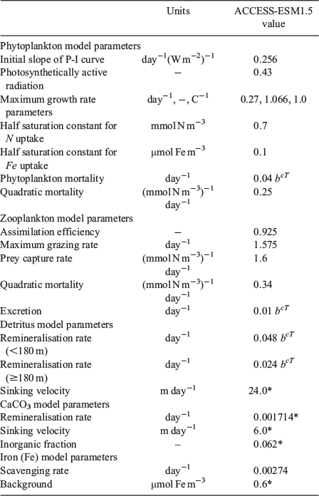
The ocean carbon cycle in ACCESS-ESM1.5 is modelled using WOMBAT (Whole Ocean Model of Biogeochemistry And Trophic-dynamics), which is described briefly here with further details in Oke et al. (2013) and Law et al. (2017). WOMBAT in ACCESS-ESM1.5 is updated to reduce bias in the carbon flux and improve the correlation of simulated nutrient and productivity fields to observations. WOMBAT is based on a NPZD cycle (nutrient–phytoplankton–zooplankton–detritus), with an added limitation from bioavailable iron. Phosphate is the major nutrient, and there is a single class of both phytoplankton and zooplankton. Carbon and oxygen cycles are coupled to the nutrient cycle via the assumed stoichiometric ratio 1:16:106:172 (P:N:C:O2). Both carbon and oxygen exchange with the atmosphere, based on wind speed squared exchange coefficients (Wanninkhof 1992). Two carbon tracers are run simultaneously: one carbon tracer exchanges with atmospheric CO2 determined by the experiment, and the second exchanges with the pre-industrial atmospheric CO2 value of 284 ppm. Two sinking tracers transport biogeochemical components out of the upper ocean: detritus for organic matter and inorganic carbonates. Biogeochemical tracers are only allowed to be positive.
Updated ocean biogeochemical (OBGC) parameters are highlighted in Table 2. Relative to the values used in ACCESS-ESM1 (Law et al. 2017), background iron and detritus sinking rates are increased to improve the OBGC state as shown and discussed in Section 7.3. The parameters related to carbonate production and export to the deep ocean are tuned so that total inorganic carbon export is ~8% of organic export (Yamanaka and Tajika 1996).
|
3 Experiments
Results presented in the following sections are based mainly on two experiments from the CMIP6 suite. Firstly, results from the 500-year pre-industrial control demonstrate the stability of the climate and biogeochemical state. The long spin-up and small drift make the ACCESS-ESM1.5 state suitable to explore modes of variability in the climate system and coupling to the carbon cycle. Secondly, the historical experiment is appropriate to compare to the climate state observed in recent decades. We also discuss the climate response to CO2 forcing based on the simulation with atmospheric CO2 increasing by 1% per year (1pctCO2) and the simulation where the concentration of atmospheric CO2 is immediately quadrupled (abrupt-4×CO2).
All experiments are run in concentration driven mode, where atmospheric CO2 concentrations are prescribed. However, land and ocean carbon fluxes have been put into passive atmospheric tracers (Law et al. 2017). These two tracers have no impact on the model simulations but allow for the atmospheric CO2 distribution to be assessed. For example, the seasonal cycle of atmospheric CO2 is strongly driven by the seasonality in land carbon fluxes. Therefore, our simulated seasonality in the historical experiment can be compared to present-day atmospheric CO2 observations.
Biogeochemistry components for land and ocean are switched on for all simulations. For the land we run with a prognostic LAI and nutrient (nitrogen and phosphorus) limitation active. The historical simulation is run with land-use change as described in Section 2.2.1.
3.1 Forcing
Forcing data generally follow that provided for CMIP6 experiments but have been re-gridded for ACCESS-ESM1.5 through a number of different methods.
The majority of forcing files have been adapted from the UK Met Office setup for CMIP6 because we share the atmospheric component (UM) for our models. However, there has been a change in the dynamics scheme between the UM version used in ACCESS-ESM1.5 and current Met Office UM configurations and this has required forcing files to be shifted by half a horizontal grid-cell. In addition, forcing fields with vertical definition such as ozone had to be interpolated from higher vertical resolution (85 levels) to our vertical resolution (38 levels).
Due to the long spin-up required and CMIP6 forcing not being available at the time, we started to spin up the model with the CMIP5 total solar irradiance (TSI) which we then also continued to use in the piControl run. The solar data in CMIP6 is quite different to CMIP5. Therefore, some adjustments had to be made for the historical and future scenarios. In the piControl run we used a TSI of 1365.65 W m−2, which is the 1850–1860 solar cycle mean in CMIP5 (Matthes et al. 2017). The CMIP6 recommendation is to use the mean of two solar cycles 1850–1872, which results in a TSI of 1360.75 W m−2. As the model uses only the TSI as input (rather than the full spectral variation), the historical and future scenario simulations used the CMIP6 data with a constant 4.9 W m−2 offset. This matches the control while giving the correct radiative forcing from the solar changes.
We also used the CMIP5 volcanic forcing (an extended version of the Sato et al. (1993) data) for our spin-up and piControl run, which specifies monthly aerosol optical depth (AOD) values in four equal latitude bands (90–30°N, 30°N–0°, 0–30°S and 30–90°S). For CMIP6, aerosol optical properties are available as a function of latitude, height and wavelength. ACCESS-ESM1.5 cannot make use of those properties, but a simple AOD at a wavelength of 550 nm is also provided for CMIP6. We used this data set to derive the AOD over our four latitude bands over the historical period. According to the CMIP6 protocol (Eyring et al. 2016) the piControl run should use the mean background volcanic aerosol during the historical simulation from 1850 to 2014. For future scenarios, the recommendation is to use the historical mean from 2025 onwards and to linearly interpolate from 2015 to 2025 (O’Neill et al. 2016). In ACCESS-ESM1.5, we use an AOD of 0.01338 for the piControl run, whereas the CMIP6 mean is 0.01067. In order to match the ACCESS-ESM1.5 piControl run, the CMIP6 values were uniformly increased by 0.00271.
ACCESS-ESM1.5 runs with nitrogen and phosphorus limitation on the land. Nitrogen deposition is provided by CMIP6 (Jones et al. 2016) and has been implemented for our simulations. Phosphorus deposition is not provided by CMIP6 and consequently we use the same phosphorus forcing as ACCESS-ESM1; the total input of phosphorus to the terrestrial biosphere in ACCESS-ESM1.5 is described in Wang et al. (2010).
4 Model spin-up
Initial conditions for the spin-up of ACCESS-ESM1.5 were derived from the end of the ACCESS-ESM1 control run.
Most of the development of the ACCESS-ESM1.5 (described in Section 2) focused on the land scheme and ocean biogeochemistry with no significant modifications to the physical climate model. The model was kept running during this phase and only restarted when developments were incrementally implemented. In this way, the climate state had the advantage of a long spin-up to approach steady state and reduce drift. Likewise, parameter tuning of CABLE (as described in Section 2.2.2) was performed during the first part of the spin-up and integrations were continued as forcing data (aerosols and radiative gases) were updated to CMIP6 standards.
In the ocean, only minor changes and bug fixes were applied to the physical model, the most significant impact came from the inclusion of Langmuir wind enhancement in the vertical mixing (Li et al. 2017), which changed the drift in the total ocean average temperature from −0.01°C per century to +0.01°C per century at the point that it was implemented (not shown). Ocean biogeochemical fields were reset to observations during the spin-up to remove biases that had built up since ACCESS-ESM1.
Overall, in the ocean and land, the physical and biogeochemical states have been integrated forward for over 3000 and 1000 years respectively, the last 600 years of which were in the finalised ACCESS-ESM1.5 configuration without any further changes to the model. We then use the state at the end of the spin-up run to initialise the piControl run.
5 Climate and carbon cycle stability
We use the 500-year piControl run to assess the stability of the climate simulation and the equilibration of the carbon cycle.
5.1 Physical climate
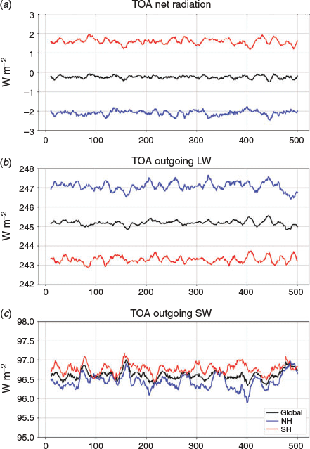
Energy should be conserved across the model. It is therefore useful to compare the top of atmosphere (TOA) radiation budget with any drift in the model simulated temperature. Fig. 4 illustrates the TOA radiation budget, with both the global mean and hemispheric mean values for the (a) net radiation, (b) outgoing longwave radiation (OLR) and (c) outgoing shortwave radiation (OSR). Results are presented as 11-year annual running means. Global mean net radiation is stable in the piControl experiment at −0.25 W m−2.
|
The hemispheric net radiation (positive downwards) values are of the correct relative order, with the NH value smaller than the global value and the southern hemisphere (SH) value larger, but with an overall greater gradient (3.69 W m−2) than that seen in present-day observations such as CERES satellite based data (1.30 W m−2) (Loeb et al. 2018). This could be due to a combination of errors in the simulation of cloud and rain interactions over the Southern Ocean as well as biases in the aerosol radiative forcing. We are also comparing the model’s pre-industrial simulated radiation to present-day CERES data, which will be different given changes in aerosols and greenhouse gases. The size and relative contributions of these problems to the net radiation requires further analysis. The relative order of the hemispheric OSR is good, with mean values close to the global mean. Hemispheric OLR values are also in the correct relative order, with NH greater than SH due to the relative size of the land areas in each hemisphere. However, the simulated NH to SH OLR gradient is larger than that seen in present-day observations (3.79 m−2 compared to 1.16 m−2).
The simulated state of the upper ocean has benefited from the long spin-up. Drift in sea surface temperature (SST) is negligible in the piControl (−8.5 × 10⁻⁵°C century−1, Fig. 5a). Time scales of the deep ocean are thousands of years, so a small drift is still present in whole ocean temperature (5.3 × 10⁻³°C century−1, Fig. 5c).

|
This whole ocean warming trend corresponds to a heat flux less than 0.02 W m−2 at the TOA so this does not contribute to the imbalance in TOA net radiation. CABLE contributes about 0.1 W m−2 to the global energy imbalance, but the source of the remainder is currently unknown.
The SST and global ocean temperature trends are also shown for the historical experiment; changes in these due to anthropogenic forcing are consistent with other ACCESS climate models (e.g. Marsland et al. 2013). Drift in sea surface salinity (SSS, 7.6 × 10⁻⁴ psu century−1 in Fig. 5b) is much less than variability. The historical response of SSS is consistent with the responses of ACCESS models in CMIP5 (Marsland et al. 2013). Drift in whole ocean salinity is 8.8 × 10⁻⁴ psu century−1 (Fig. 5d) is more evident since variability is negligible. The response of the historical total salinity is consistent with the changes in ocean volume. The linear trend in global salinity indicates that ACCESS-ESM1.5 still has the same discrepancy in coupling water, related to use freshwater mass fluxes in a volume-conserving model, as discussed in Marsland et al. (2013).
Circulation of the ocean is also stable (Fig. 5e, f). Centennial scale variability in the Antarctic Circumpolar Current at Drake Passage is evident and is weakly correlated in the rate of Antarctic Bottom Water formation (estimated as the minimum in the overturning cell at 30°S). Historical trends are lower in both these circulation metrics shown; however, further analysis would be required to clarify how much of this is natural variability or a forced response.
Trends in sea-ice extent (area with at least 15% cover) are stable in the control for both hemispheres (Fig. 5g, h). Although there is clear evidence of a decrease in Arctic sea-ice in the last decades of the historical experiment, Antarctic sea-ice is still within the range of decadal variability of the piControl.
5.2 Carbon cycle
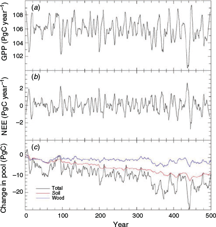
The aim of the spin-up is to get the model into equilibrium, aiming for a mean net-zero flux of carbon to the atmosphere. During the control run this should remain stable without any further drifts, although this may be hard to achieve due to long turnover times in the slow soil carbon pools and the millennium time-scale of deep ocean circulation. For land carbon, both GPP and NEE are stable across the piControl run (Fig. 6a, b).
|
Temporal variability in NEE is driven by variability in GPP with years of lower GPP being a carbon source to the atmosphere while higher GPP leads to a carbon sink. The mean NEE in ACCESS-ESM1 was about 0.14 PgC year−1 over the last 500 years of the control run. However, at the PFT level, some vegetation types were still showing relatively large drifts of opposite signs (Law et al. 2017, Fig. 6a). Solving the issues we had with the carbon conservation and extending the spin-up for ACCESS-ESM1.5 has led to a significant improvement in NEE. The mean NEE for the control run in ACCESS-ESM1.5 is 0.02 PgC year−1 over the 500 years. At the PFT level, all vegetation types are close to zero (ranging from –0.002 to 0.006 PgC year−1) with no significant trends.
Over the 500-year control run, total land carbon stocks decreased by about 12 PgC (Fig. 6c), which is about 0.02 PgC year−1. This matches the NEE over the same period, indicating that the issues with the carbon conservation prominent in ACCESS-ESM1 have been solved. Changes in the total carbon are dominated by changes in the slowest soil carbon pools (i.e. passive pool) with a smaller contribution from the plant wood pool. The plant root pool (not shown) contributes to the interannual variability in the total land pool size.
Nitrogen stocks are also decreasing slightly in the control run with a total loss of about 1.5 PgN over 500 years. Again, this is dominated by changes in the slowest soil nitrogen pools. Phosphorus pools behave slightly differently. Although we observe an overall loss of about 0.5 PgP over the length of the control run, the passive soil pool is increasing (about 0.08 PgP), whereas the other soil pools are decreasing in size.
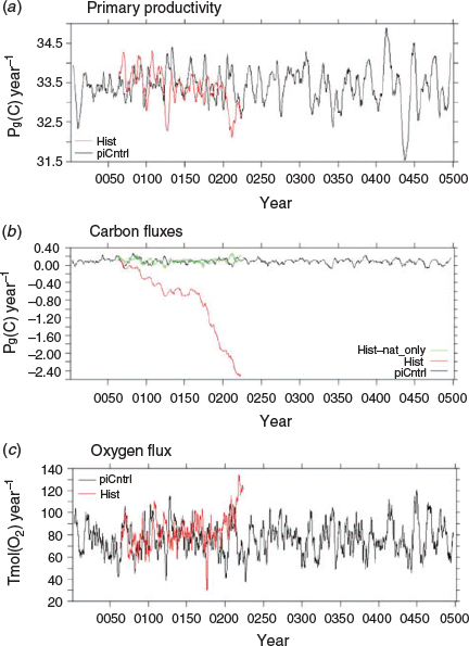
The ocean biogeochemical state in ACCESS-ESM1.5 has benefited from both the long spin-up and updates since ACCESS-ESM1, as seen in the stability of the OBGC fluxes shown in Fig. 7.
|
Average total ocean productivity, or the uptake of carbon driven by photosynthesis, is 33.5 PgC year−1 with a negligible drift of –0.0163 PgC year−1 per century. The ocean productivity in ACCESS-ESM1 was ~51 PgC year−1, which compared well with global estimates (45–50 PgC year−1, Carr et al. 2006). The ACCESS-ESM1.5 productivity is lower but still reasonable, since a significant fraction of the estimated productivity is from coastal and marginal seas with processes that WOMBAT does not resolve, such as sources from rivers. There is an indication of a reduction in ocean productivity towards the end of the ACCESS-ESM1.5 historical experiment, but the change is still within the range of variability of the piControl.
The average piControl sea–air carbon flux of ACCESS-ESM1.5 is 0.080 PgC year−1, representing a significant improvement in the bias from the previous version (ACCESS-ESM1, 0.6 PgC year−1; Law et al. 2017). The drift in this carbon flux is −0.0048 PgC year−1 per century in the piControl. The natural carbon flux in the historical experiment (Fig. 7b) stays within the range of variability of the piControl, and total carbon flux responds to increase in atmospheric CO2 reaching an uptake of ~2.5 PgC at the end of the historical period, consistent with ocean fluxes estimated from the Global Carbon Project (Le Quéré et al. 2015). Oxygen flux is spun-up and stable in the piControl, with a drift of −0.153 Tmol(O2)year−1 per century; the average flux is non-zero (−76.4 Tmol(O2) year−1) due to remineralisation of detritus in oxygen minimum zones, such as the eastern Equatorial Pacific. Remineralisation normally consumes oxygen from the ocean interior; however, WOMBAT does not allow tracers to go negative nor handle denitrification, hence these zones can act as a net source of oxygen. The bias of –76.4 Tmol(O2) year−1 corresponds to 0.6 PgC year−1, a small fraction of the ocean productivity. There is a clear increase in the oxygen trend in the last decade of the historical experiment, outside the range of variability from the piControl. This extra outgassing of oxygen coincides with higher SST that increases oxygen partial pressure.
6 Climate sensitivity
The climate response (surface warming) to CO2 forcing can be derived from the CMIP6 DECK simulations, 1pctCO2 and abrupt-4×CO2. Here, we focus on the equilibrium climate sensitivity (ECS) and the transient climate response (TCR).
6.1 Equilibrium climate sensitivity
The ECS is defined as the amount of global mean surface warming resulting from a doubling of CO2 once equilibrium has been achieved (Knutti and Hegerl 2008). Since reaching equilibrium can take a long time (i.e. several thousand years), Gregory et al. (2004) proposed estimating climate sensitivity from the correlation of temperature and energy balance changes, which does not require the model to be at equilibrium. This method involves an instantaneous quadrupling of CO2 concentration which is then held fixed for 150 years. This method assumes that the response to a constant radiative forcing F is a linear relation between the change in the TOA net energy flux N, and the change in the surface air temperature ΔT, N = F − αΔT, with α (W m−2 °C−1) the climate feedback parameter. Regressing N and ΔT provides an estimate of both the radiative forcing F and α. Note that the forcing calculated here is not the pure CO2 radiative forcing because it includes short-term atmospheric adjustments other than the stratospheric equilibration (Gregory and Webb 2008). For ACCESS-ESM1.5, the result of applying this method of calculation is an estimated ECS of 3.87°C, which is similar to the ECS in ACCESS-ESM1 (3.78°C).
6.2 Transient climate response
The TCR is derived from the 1pctCO2 experiment, where atmospheric CO2 concentrations are increased by 1% per year over a 150-year period. It is calculated as the difference in surface air temperature between the piControl run and the 20-year mean centred on the year of CO2 doubling (year 70). For ACCESS-ESM1.5 the TCR is 1.95°C, which is slightly larger than the TCR in ACCESS-ESM1 (1.83°C).
7 Present-day climatology
The present-day climatology is assessed using the later part of the 1850–2014 historical simulation. Different comparison periods are used, depending on whether we are comparing with observations only or whether we include ACCESS-ESM1 results which were previously analysed for the 1986–2005 period (Ziehn et al. 2017).
7.1 Physical climate
Fig. 8 shows the biases of surface temperature and salinity (averaged over 1975 to 2014) with respect to the Hadley Centre Sea Ice and Sea Surface Temperature data set (HadISST) from these years (Rayner et al. 2003) and World Ocean Atlas (WOA, Antonov et al. 2010). Spatial patterns in the biases are very similar to those of ACCESS1.3 (Bi et al. 2013), confirming that the minor updates in ACCESS-ESM1 and ACCESS-ESM1.5 have had negligible impact on the simulated climate. In Fig. 8a, warm SST biases exist in western boundary current regions such as the Kurioshio and Gulf Stream where there are strong spatial gradients in temperature associated with mesoscale dynamics that are not explicitly simulated in a 1-degree ocean model. The Southern Ocean is also too warm, like ACCESS1.3 and ACCESS-ESM1 where the summer mixed layer is too shallow and too warm, as discussed in Ziehn et al. (2017). Warm biases are also found in upwelling regions on eastern boundaries of ocean basins, for example the Humboldt Current (Peru) and the Benguela Current (Africa). These biases are associated with ocean and atmospheric dynamics in the coastal regions that are not resolved in most climate models (Richter 2015).

|
Sea surface salinity biases of ACCESS-ESM1.5 (Fig. 8) are very similar to ACCESS1.3 (Bi et al. 2013). Most significant biases are marginal seas: the Mediterranean, Bay of Bengal and the Siberian Arctic coast have high salinity and low values occur in the Yellow Sea, Sea of Japan and Hudson Bay.
The sea-ice model set up in ACCESS-ESM1.5 is unmodified from ACCESS-ESM1 and the ice extent is consistent with previous results, ACCESS-ESM1 (Law et al. 2017) and ACCESS1.3 (Marsland et al. 2013; Uotila et al. 2013). ACCESS-ESM1.5 sea-ice climatologies are the same as prognostic LAI versions of ACCESS-ESM1 in the south but slightly higher in the north due to updates to the land model which reduced LAI and cooled the climate in this region. Fig. 8c, d shows climatologies of sea-ice extent (area with at least 15% ice cover) from ACCESS-ESM1.5 piControl and historical experiments, relative to observed climatologies (Fetterer et al. 2017), based on years 1981–2010. Both piControl and historical climatologies of Antarctic sea-ice are within ~1 × 10¹² m2 of observed extents throughout the seasonal cycle. The historical climatology of Arctic sea-ice is less than the piControl, consistent with the trends in Fig. 5h and closer to observed extents (within ~0.5 × 10¹² m2 across the seasons).
A measure of potential model bias is gained from comparing the model’s mean surface temperature to ERA-Interim (Dee et al. 2011), with seasonal mean biases illustrated in Fig. 9a, b.

|
Overall, the biases are very similar to those found for ACCESS1.3 in Kowalczyk et al. (2013) (Fig. 10c, d). There is a Southern Ocean warm bias in both seasons, continuing a longstanding issue with the atmospheric model. The June–August warm bias is more evident over India than for December–February. There are also signs of warm biases across the equatorial land masses including the Maritime continent along with central North America. The northern continental biases appear to be slightly larger than in ACCESS1.3. Cool biases occur over North Africa and the Arabian Peninsula, particularly in December–February.

|
The atmospheric zonal mean temperature (Fig. 10) has the expected structure, warm over the equator at low altitudes, becoming cooler towards the poles and higher in the atmosphere to very cold in the stratosphere above the Antarctic and equator. Biases relative to ERA-Interim (Fig. 10b–d) indicate some issues around Antarctica and with the polar jet regions which are cooler in December–February (and hence slower) than in the reanalysis (not shown).
The simulated and observed global precipitation are compared in Fig. 9c, d. The largest biases occur in the region of the Intertropical Convergence zone where some of the tropical regions are too dry while others are too wet, with some seasonal variations. There is a general tendency towards a wet bias over the Maritime continent. India shows a rainfall deficit in June– August, consistent with the temperature bias noted above. Again, the biases appear to be similar to those from ACCESS1.3 (Kowalczyk et al. 2013). The annual global mean precipitation for ACCESS-ESM1.5 piControl is 3.21 mm day−1, which is somewhat higher than the GPCP (Adler et al. 2003) observational estimate of 2.68 mm day−1 for 1979–1998. Higher simulated rainfall with the UM and other global atmospheric models is a longstanding issue.
7.2 Land carbon
In this section we evaluate the land carbon cycle against observation-based estimates and also compare against ACCESS-ESM1 results. For the analysis we use a 20-year period (1986–2005) from the historical simulation and for the observations, unless stated otherwise. The following data products are used:
GPP: global gridded GPP (0.5° resolution) based on up-scaled flux network data provided by Jung et al. (2011).
LAI: global gridded LAI (1/12° resolution) based on Moderate Resolution Imaging Spectroradiometer (MODIS) and Advanced Very High-Resolution Radiometer (AVHRR) data provided by Zhu et al. (2013).
CO2 concentrations: mean atmospheric CO2 seasonal cycles derived from NOAA/Earth System Research Laboratory (ESRL) flask samples as processed in the GLOBALVIEW data product (GLOBALVIEW-CO2 2013).
Table 1 presents the mean prognostic LAI for each PFT for ACCESS-ESM1 and ACCESS-ESM1.5, including the relative change in amplitude over the last 20 years of the historical period. Consistent with the parameter changes (also shown in Table 1) we observe the largest change in mean LAI and relative amplitude for C4 grass. This has a large impact on the LAI in the tropical region as shown in Fig. 11d. With ACCESS-ESM1, we underestimated the LAI in the Tropics (mean 1.5), mainly because the LAI for C4 grass was very small. ACCESS-ESM1.5 results (mean 2.0) are much closer to the observed LAI (mean 2.3) in this region.

|
In the northern extra-tropics (i.e. 20−90°N, Fig. 11c) the LAI in ACCESS-ESM1.5 has also improved, the mean value of 1.3 (1.8 in ACCESS-ESM1) is now closer to the observed value of 0.9, mainly due to a reduction in LAI for evergreen needleleaf forest. However, it needs to be noted that the observations are based on satellite data which do not account for vegetation that is covered by snow in the mid to high northern latitudes during the winter months. This might be why the seasonality in the observations is stronger with a LAI close to zero during the NH winter. The shift in the peak value between the observations (July) and the model (August) is probably due to the prescribed phenology (timing of leaf onset and fall) used in both ACCESS-ESM versions (Law et al. 2017).
The LAI in the SH (i.e. 20−90°S, Fig. 11b) has slightly worsened in ACCESS-ESM1.5. This can be attributed to the fact that the parameter tuning was performed at the PFT level and not at the regional/latitudinal level. However, the land fraction in the SH is small in comparison to the other latitudinal bands assessed here and therefore the impact at the global scale is thought to be small.
The global seasonal cycle of LAI (Fig. 11a) is mainly influenced by the northern extra-tropics. With ACCESS-ESM1 we overestimate the LAI (mean 1.7) by a significant amount, whereas with ACCESS-ESM1.5 (mean 1.5) we are very close to the observed global mean of 1.4.
The parameter tuning and changes in LAI also impact GPP. The ACCESS-ESM1.5 run provides a mean GPP of about 124 PgC year−1, which agrees well with observation-based estimates from other studies: 123 ± 8 PgC year−1 (Beer et al. 2010) and 121 PgC year−1 with a 95% confidence interval of 110–130 PgC year−1 (Ziehn et al. 2011). In ACCESS-ESM1, the GPP was somewhat higher at around 130 PgC year−1. The difference in the spatial distribution of GPP between observations (Jung et al. 2011) and the two ACCESS-ESM versions is presented in Fig. 12.

|
The NH boreal region is less productive in ACCESS-ESM1.5 and closer to the observations. Productivity in South America has increased in ACCESS-ESM1.5, which also leads to a better agreement with the observations. At the same time the increase in GPP in Central Africa simulated with ACCESS-ESM1.5 is too large in comparison with the observations. We also note that productivity in South-East Australia is somewhat higher than observations suggest. In this global configuration of CABLE, trees in South-East Australia are classified as evergreen broadleaf, which is also used for tropical forests. It is likely that the parameter values used for evergreen broadleaf trees are better suited to tropical forests than Australian eucalypt forests and consequently result in larger productivity than observed.
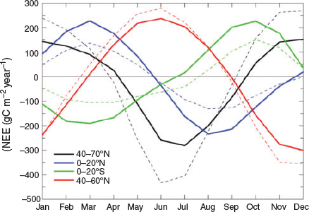
The carbon uptake by the land (NEE) varies throughout the year, with the largest uptake during the plant growing season. This is captured well by the model as shown in Fig. 13. In ACCESS-ESM1, seasonality was largest in the NH (about 600 gC m−2 year−1 peak-to-peak), whereas in ACCESS-ESM1.5 this has almost halved (about 325 gC m−2 year−1 peak-to-peak) most likely due to a reduced productivity based on the new parametrisation for photosynthesis. The tropics, however, show a large increase in seasonality, presumably for the same reason. The seasonal cycle of the land uptake for the SH is almost unchanged.
|
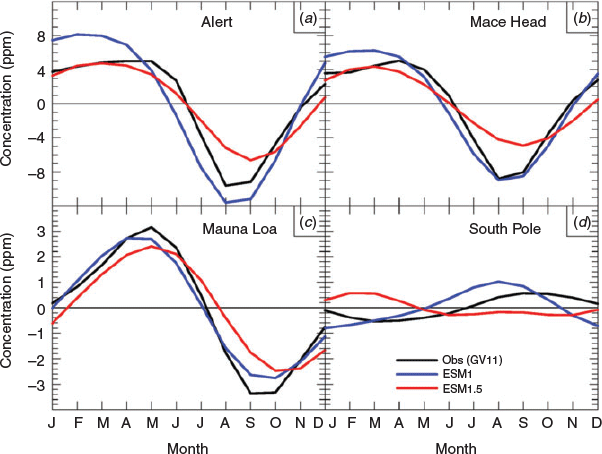
The changes in the seasonal land uptake will also impact the seasonal amplitude in atmospheric CO2 concentrations, which is presented for four different stations in Fig. 14. The monthly CO2 timeseries (using land and ocean CO2 fluxes) from the appropriate model grid-cell is fitted with a quadratic (to represent the trend in CO2) and a series of harmonics. The harmonics are used to represent the seasonal cycle. In ACCESS-ESM1, the seasonal amplitude for stations in the high northern latitudes (i.e. Alert, 82°N) was overestimated by a significant amount. In ACCESS-ESM1.5, we underestimate the seasonal cycle, but are closer to observations in the NH winter. The minimum concentrations also occur up to a month later than observed. For Mace Head (53°N, Fig. 14b) the seasonal amplitude is also underestimated by ACCESS-ESM1.5, compared to a slight overestimate in ACCESS-ESM1. However, the results for this site are sensitive to the grid-cell sampled from the model. Here we have shown the grid-cell to the west of Mace Head because flask sampling at the site would occur when the winds are from the ocean sector, i.e. westerly. We would expect that this would give a lower amplitude signal than a grid-cell with a large land influence. This is the case in ACCESS-ESM1.5 but not in ACCESS-ESM1, where lower concentrations appear to be transported from the north. The seasonal amplitude for Mauna Loa (20°N) is reasonably similar for the two model versions and both slightly underestimate the observed amplitude (Fig. 14c). As at Alert and Mace Head, ACCESS-ESM1.5 shows a phase lag relative to the observations and ACCESS-ESM1. The small seasonal cycle at the South Pole (Fig. 14d) is more challenging to simulate because ocean and land fluxes both make significant contributions. The peak-to-peak values are well captured by the model, but the seasonality using ACCESS-ESM1.5 is opposite to what the observations suggest.
|
7.3 Ocean biogeochemistry
Fig. 15 shows surface maps of biogeochemical fields – ocean productivity, nutrients and CO2 fluxes – averaged from years 1996–2005 of historical experiments with ACCESS-ESM1 (left column) and ACCESS-ESM1.5 (middle), that are compared to observations (right, Behrenfeld and Falkowski 1997; Garcia et al. 2010a; Takahashi et al. 2009). These years are common to the ACCESS-ESM1 (CMIP5) and ACCESS-ESM1.5 (CMIP6) historical experiments and are centred on the year of carbon flux observation product used as reference, noting that CO2 flux has a strong historical trend due to direct response to atmospheric anthropogenic CO2. Updates to the OBGC parameters in ACCESS-ESM1.5 described in Section 2.3.1 and Table 2 have greatly improved the comparison to observations, for instance, in ACCESS-ESM1 nutrients upwelled in the Equatorial Pacific were spread extensively across the tropics (Fig. 15d) which are now much more realistic in ACCESS-ESM1.5 (Fig. 15e). Higher values of specified background iron have increased the biological uptake of nutrients at the sites of upwelling, and increasing the sinking of detritus has reduced nutrient recycling and lateral spread across the Pacific. Surface distributions of ACCESS-ESM1.5 nutrients correlate better to the WOA (correlation coefficient 0.89) relative to ACCESS-ESM1 (0.68). The distribution of biological production in ACCESS-ESM1.5 has also improved. The decreased nutrient extent in ACCESS-ESM1.5 has reduced the productivity in the Western Pacific Warm Pool, which was unrealistically high in ACCESS-ESM1 (Fig. 15a). High background iron in ACCESS-ESM1.5 also increases productivity along the southern subtropical front (40–45°S), which was low in ACCESS-ESM1. This subtropical front is also a region of CO2 uptake in ACCESS-ESM1.5 and observations (Fig. 15h, i) that were weak in ACCESS-ESM1 (Fig. 15g). Elsewhere, OBGC parameter updates have had little impact on the carbon flux, the overall distribution of CO2 flux is very similar to ACCESS-ESM1, consistent with the same physical circulation in each model.

|
The distributions of OBGC tracers in the ocean interior are shown in Fig. 16, which are zonal means (averaged from the same years of historical experiments from ACCESS-ESM1 and ACCESS-ESM1.5 used in Fig. 15) compared to observations (Garcia et al. 2010a, 2010b; Key et al. 2004). The alkalinity section (Fig. 16b) is still biased low in the upper ocean and high in the deep. However, these biases are have been reduced, for instance, the average alkalinity at 500 m in ACCESS-ESM1.5 (2351 mmol m−3) is closer to observations (2379 mmol m−3, Key et al. 2004) than alkalinity here in ACCESS-ESM1 (2340 mmol m−3, Fig. 16a). Phosphate is biased high in the upper 1000 m in tropical regions (Fig. 16e), as for ACCESS-ESM1 (Fig. 16d). Updates to the OBGC have deepened the remineralisation, which has reduced the ACCESS-ESM1 nutrient deficiency in the abyssal waters in the northern and tropical oceans, and also reduced the oxygen bias here (Fig. 16h). However, the Southern Ocean is still low in nutrients and missing the ‘nutrient trapping’ observed, the combined effect of ocean circulation and the biological pump to enhance nutrients here (Fig. 16d, e). There is more productivity and export in the ACCESS-ESM1.5 Southern Ocean, which has reduced the oxygen bias at depth. Oxygen was ~320 mmol(O2) m−3 in the ACCESS-ESM1 Southern Ocean, this is reduced to ~280 mmol(O2) m−3 in ACCESS-ESM1.5 but is still higher than observations (~240 mmol(O2) m−3). This excess oxygen relative to observations may be due a weak Southern Ocean biological pump or excessive ventilation of the Southern Ocean; the actual cause has not yet been resolved.

|
Unrealistic values of alkalinity are found in the Red Sea (not shown) – maximum values of over 20 000 mmol m−3 – due to poor mixing in this marginal sea. The physical ocean model has extra horizontal mixing of salinity in this region to avoid extreme salinities. However, this mixing has yet to be applied to OBGC tracers (nutrients are also affected), hence there is a break in the alkalinity–salinity relationship. This is a local effect that does not impact global results.
8 Summary and conclusions
ACCESS-ESM1.5 has been developed by CSIRO mainly for the purpose of contributing to CMIP6 with a model version that includes the carbon cycle. ACCESS-ESM1.5 will also provide the capability to answer key science questions around climate change mitigation, particularly where it is important to account for feedbacks between the carbon cycle and climate. ACCESS-ESM1.5 can be used to explore how climate change might impact Australia’s productivity, resource usage and resilience in a global context, while providing a baseline case for experiments that use CABLE in configurations that are designed for Australian applications.
As an earth system model, ACCESS-ESM1.5 includes biogeochemical components for the land and the ocean to simulate the global carbon cycle. The biogeochemical component for the land, CASA-CNP, allows for nutrient limitation through the implementation of a nitrogen and phosphorus cycle. Although the number of participating ESMs has increased drastically in CMIP6, there are very few ESM contributions from the SH. ACCESS-ESM1.5 is one of those very few. In addition, ACCESS-ESM1.5 is probably the only CMIP6 model with phosphorus limitation on the land, highlighting its unique status.
The ACCESS-ESM1.5 submission to CMIP6 will consist of core experiments and mainly Tier 1 experiments for the following MIPs: ScenarioMIP, C4MIP, CDRMIP, RFMIP, ZECMIP and PMIP (through collaboration with the University of New South Wales). The long spin-up (several thousand years) results in a stable climate state, negligible drifts in temperature and net carbon fluxes that are close to zero. This highlights the suitability of ACCESS-ESM1.5 to explore modes of variability in the climate system and coupling to the carbon cycle. Validation over the historical period against observations shows good agreement and also significant improvements over the previous version, ACCESS-ESM1. This makes ACCESS-ESM1.5 a useful tool to explore future land and ocean carbon uptake and mitigation scenarios. The climate response in ACCESS-ESM1.5 to CO2 has been estimated as 3.87°C (ECS), based on the abrupt-4xCO2 simulation. This is closer to the higher bound in comparison to CMIP5 model results (24 multi-model average of 3.36°C, standard deviation 0.75°C), but only moderate in comparison to recent CMIP6 model results.
Conflicts of interest
The authors declare no conflicts of interest.
Acknowledgements
We acknowledge the World Climate Research Programme, which, through its Working Group on Coupled Modelling, coordinated and promoted CMIP6. We thank the Earth System Grid Federation (ESGF) for archiving the data and providing access, and the multiple funding agencies who support CMIP6 and ESGF. ACCESS-ESM1.5 work is jointly funded through CSIRO and the Earth Systems and Climate Change Hub of the Australian Government’s National Environmental Science Program. ACCESS-ESM1.5 simulations and data processing were undertaken with the assistance of resources from the National Computational Infrastructure (NCI Australia), an NCRIS enabled capability supported by the Australian Government.
References
Antonov, J. I., Seidov, D., Boyer, T. P., Locarnini, R. A., Mishonov, A. V., Garcia, H. E., Baranova, O. K., Zweng, M. M., and Johnson, D. R. (2010). World Ocean Atlas 2009, Volume 2: Salinity. In ‘NOAA Atlas NESDIS 69’. (Ed. S. Levitus.) 184 pp. (U.S. Government Printing Office: Washington, D.C.)Beer, C., Reichstein, M., Tomelleri, E., Ciais, P., Jung, M., Carvalhais, N., Rödenbeck, C., Arain, M. A., Baldocchi, D., Bonan, G. B., Bondeau, A., Cescatti, A., Lasslop, G., Lindroth, A., Lomas, M., Luyssaert, S., Margolis, H., Oleson, K. W., Roupsard, O., Veenendaal, E., Viovy, N., Williams, C., Woodward, F. I., and Papale, D. (2010). Terrestrial Gross Carbon Dioxide Uptake: Global Distribution and Covariation with Climate. Science 329, 834–838.
| Terrestrial Gross Carbon Dioxide Uptake: Global Distribution and Covariation with Climate.Crossref | GoogleScholarGoogle Scholar | 20603496PubMed |
Behrenfeld, M. J., and Falkowski, P. G. (1997). Photosynthetic rates derived from satellite-based chlorophyll concentration. Limnology and Oceanography 42, 1–20.
| Photosynthetic rates derived from satellite-based chlorophyll concentration.Crossref | GoogleScholarGoogle Scholar |
Bi, D., Dix, M., Marsland, S., O’Farrell, S., Sullivan, A., Bodman, R., Law, R., Harman, I., Srbinovsky, J., Rashid, H., Dobrohotoff, P., Mackallah, C., Yan, H., Hirst, A., Savita, A., Dias, F. B., Woodhouse, M., Fiedler, R., and Heerdegen, A. (2020). Configuration and spin-up of ACCESS-CM2, the new generation Australian Community Climate and Earth System Simulator Coupled Model. J. South. Hemisph. Earth Sys. Sci. , .
| Configuration and spin-up of ACCESS-CM2, the new generation Australian Community Climate and Earth System Simulator Coupled Model.Crossref | GoogleScholarGoogle Scholar |
Bi, D., Dix, M., Marsland, S. J., O’Farrell, S., Rashid, H. A., Uotila, P., Hirst, A. C., Kowalczyk, E., Golebiewski, M., Sullivan, A., Yan, H., Hannah, N., Franklin, C., Sun, Z., Vohralik, P., Watterson, I., Zhou, X., Fiedler, R., Collier, M., Ma, Y., Noonan, J., Stevens, L., Uhe, P., Zhu, H., Griffies, S. M., Hill, R., Harris, C., and Puri, K. (2013). The ACCESS coupled model: description, control climate and evaluation. Aus. Meteor. Oceanogr. J. 63, 41–64.
| The ACCESS coupled model: description, control climate and evaluation.Crossref | GoogleScholarGoogle Scholar |
Carr, M.-E., Friedrichs, M. A. M., Schmeltz, M., Aita, M. N., Antoine, D., Arrigo, K. R., Asanuma, I., Aumont, O., Barber, R., Behrenfeld, M., Bidigare, R., Buitenhuis, E., Campbell, J., Ciotti, A., Dierssen, H., Dowell, M., Dunne, J., Esaias, W., Gentili, B., Gregg, W., Groom, S., Hoepffner, N., Ishizaka, J., Kameda, T., Le Quéré, C., Lohrenz, S., Marra, J., Mélin, F., Moore, J., Morel, A., Reddy, T. E., Ryan, J., Scardi, M., Smyth, T., Turpie, K., Tilstone, G., Waters, K., and Yamanaka, Y. (2006). A comparison of global estimates of marine primary production from ocean color. Deep-Sea Research II 53, 741–770.
| A comparison of global estimates of marine primary production from ocean color.Crossref | GoogleScholarGoogle Scholar |
Corbin, K. D. and Law, R. M. (2011). Extending atmospheric CO2 and tracer capabilities in ACCESS, CAWCR Technical Report 035, CSIRO/Bureau of Meteorology, Aspendale, Victoria. Available at https://www.cawcr.gov.au/technical-reports/CTR_035.pdf.
Craig, A., Valcke, S., and Coquart, L. (2017). Development and performance of a new version of the OASIS coupler, OASIS3-MCT_3.0. Geosci. Model Dev. 10, 3297–3308.
| Development and performance of a new version of the OASIS coupler, OASIS3-MCT_3.0.Crossref | GoogleScholarGoogle Scholar |
Dee, D. P., Uppala, S. M., Simmons, A. J., Berrisford, P., Poli, P., Kobayashi, S., Andrae, U., Balmaseda, M. A., Balsamo, G., Bauer, P., Bechtold, P., Beljaars, A. C. M., van de Berg, L., Bidlot, J., Bormann, N., Delsol, C., Dragani, R., Fuentes, M., Geer, A. J., Haimberger, L., Healy, S. B., Hersbach, H., Hólm, E. V., Isaksen, L., Kållberg, P., Köhler, M., Matricardi, M., McNally, A. P., Monge-Sanz, B. M., Morcrette, J.-J., Park, B.-K., Peubey, C., de Rosnay, P., Tavolato, C., Thépaut, J.-N., and Vitart, F. (2011). The ERA-Interim reanalysis: configuration and performance of the data assimilation system. Quart. J. Roy. Meteorol. Soc. 137, 553–597.
| The ERA-Interim reanalysis: configuration and performance of the data assimilation system.Crossref | GoogleScholarGoogle Scholar |
Eyring, V., Bony, S., Meehl, G. A., Senior, C. A., Stevens, B., Stouffer, R. J., and Taylor, K. E. (2016). Overview of the Coupled Model Intercomparison Project Phase 6 (CMIP6) experimental design and organization. Geosci. Model Dev. 9, 1937–1958.
| Overview of the Coupled Model Intercomparison Project Phase 6 (CMIP6) experimental design and organization.Crossref | GoogleScholarGoogle Scholar |
Fetterer, F., Knowles, K., Meier, W. N., Savoie, M., and Windnagel, A. K. (2017). Sea Ice Index, Version 3. NSIDC: National Snow and Ice Data Center, Boulder, Colorado USA
Fung, I. Y., Doney, S. C., Lindsay, K., and John, J. (2005). Evolution of carbon sinks in a changing climate. Proc. Natl. Acad. Sci. USA 102, 11201–11206.
| Evolution of carbon sinks in a changing climate.Crossref | GoogleScholarGoogle Scholar | 16061800PubMed |
Garcia, H. E., Locarnini, R. A., Boyer, T. P., Antonov, J. I., Zweng, M. M., Baranova, O. K., and Johnson, D. R. (2010a). World Ocean Atlas 2009, Volume 4: Nutrients (phosphate, nitrate, silicate). In ‘NOAA Atlas NESDIS 71’. (Ed. S. Levitus.) 398 pp. (U.S. Government Printing Office: Washington, D.C.)
Garcia, H. E., Locarnini, R. A., Boyer, T. P., Antonov, J. I., Baranova, O. K., Zweng, M. M., and Johnson, D. R. (2010b). World Ocean Atlas 2009, Volume 3: Dissolved Oxygen, Apparent Oxygen Utilization, and Oxygen Saturation. In ‘NOAA Atlas NESDIS 70’. (Ed. S. Levitus.) 344 pp. (U.S. Government Printing Office: Washington, D.C.)
GLOBALVIEW-CO2: Cooperative Global Atmospheric Data Integration Project. (2013), updated annually. Multi-laboratory compilation of synchronized and gap-filled atmospheric carbon dioxide records for the period 1979-2012. NOAA, Boulder, CO
Gregory, J., and Webb, M. (2008). Tropospheric Adjustment Induces a Cloud Component in CO2 Forcing. J. Climate 21, 58–71.
| Tropospheric Adjustment Induces a Cloud Component in CO2 Forcing.Crossref | GoogleScholarGoogle Scholar |
Gregory, J. M., Ingram, W. J., Palmer, M. A., Jones, G. S., Stott, P. A., Thorpe, R. B., Lowe, J. A., Johns, T. C., and Williams, K. D. (2004). A new method for diagnosing radiative forcing and climate sensitivity. Geophys. Res. Lett. 31, .
| A new method for diagnosing radiative forcing and climate sensitivity.Crossref | GoogleScholarGoogle Scholar |
Griffies, S. M. (2009). Elements of MOM4p1, GFDL Ocean Group Tech. Rep. No. 6. NOAA/Geophysical Fluid Dynamics Laboratory.
Griffies, S. M. (2012). Elements of MOM5, GFDL Ocean Group Tech. Rep. No. 7. NOAA/Geophysical Fluid Dynamics Laboratory.
Hewitt, H. T., Copsey, D., Culverwell, I. D., Harris, C. M., Hill, R. S. R., Keen, A. B., McLaren, A. J., and Hunke, E. C. (2011). Design and implementation of the infrastructure of HadGEM3: the next-generation Met Office climate modelling system. Geosci. Model Dev. 4, 223–253.
| Design and implementation of the infrastructure of HadGEM3: the next-generation Met Office climate modelling system.Crossref | GoogleScholarGoogle Scholar |
Hunke, E. C. and Lipscomb, W. H. (2010). CICE: The Los Alamos sea ice model documentation and software user’s manual, Version 4.1, LA-CC06-012. Los Alamos National Laboratory, NM.
Hurtt, G., Chini, L., Sahajpal, R., Frolking, S., Bodirsky, B. L., Calvin, K., Doelman, J., Fisk, J., Fujimori, S., Goldewijk, K. K., Hasegawa, T., Havlik, P., Heinimann, A., Humpenöder, F., Jungclaus, J., Kaplan, J., Krisztin, T., Lawrence, D., Lawrence, P., Mertz, O., Pongratz, J., Popp, A., Riahi, K., Shevliakova, E., Stehfest, E., Thornton, P., van Vuuren, D., and Zhang, X. (2017). Harmonization of global land use scenarios (LUH2): Historical v2.1h 850–2015 , .
| Harmonization of global land use scenarios (LUH2): Historical v2.1h 850–2015Crossref | GoogleScholarGoogle Scholar | 28921829PubMed |
Jones, C. D., Arora, V., Friedlingstein, P., Bopp, L., Brovkin, V., Dunne, J., Graven, H., Hoffman, F., Ilyina, T., John, J. G., Jung, M., Kawamiya, M., Koven, C., Pongratz, J., Raddatz, T., Randerson, J. T., and Zaehle, S. (2016). C4MIP – The Coupled Climate–Carbon Cycle Model Intercomparison Project: experimental protocol for CMIP6. Geosci. Model Dev. 9, 2853–2880.
| C4MIP – The Coupled Climate–Carbon Cycle Model Intercomparison Project: experimental protocol for CMIP6.Crossref | GoogleScholarGoogle Scholar |
Jones, C. D., Frölicher, T. L., Koven, C., MacDougall, A. H., Matthews, H. D., Zickfeld, K., Rogelj, J., Tokarska, K. B., Gillett, N. P., Ilyina, T., Meinshausen, M., Mengis, N., Séférian, R., Eby, M., and Burger, F. A. (2019). The Zero Emissions Commitment Model Intercomparison Project (ZECMIP) contribution to C4MIP: quantifying committed climate changes following zero carbon emissions. Geosci. Model Dev. 12, 4375–4385.
| The Zero Emissions Commitment Model Intercomparison Project (ZECMIP) contribution to C4MIP: quantifying committed climate changes following zero carbon emissions.Crossref | GoogleScholarGoogle Scholar |
Jung, M., Reichstein, M., Margolis, H. A., Cescatti, A., Richardson, A. D., Arain, M. A., Arneth, A., Bernhofer, C., Bonal, D., Chen, J., Gianelle, D., Gobron, N., Kiely, G., Kutsch, W., Lasslop, G., Law, B. E., Lindroth, A., Merbold, L., Montagnani, L., Moors, E. J., Papale, D., Sottocornola, M., Vaccari, F., and Williams, C. (2011). Global patterns of land-atmosphere fluxes of carbon dioxide, latent heat, and sensible heat derived from eddy covariance, satellite, and meteorological observations. J. Geophys. Res. Biogeosci. 116, G00J07.
| Global patterns of land-atmosphere fluxes of carbon dioxide, latent heat, and sensible heat derived from eddy covariance, satellite, and meteorological observations.Crossref | GoogleScholarGoogle Scholar |
Kageyama, M., Braconnot, P., Harrison, S. P., Haywood, A. M., Jungclaus, J. H., Otto-Bliesner, B. L., Peterschmitt, J.-Y., Abe-Ouchi, A., Albani, S., Bartlein, P. J., Brierley, C., Crucifix, M., Dolan, A., Fernandez-Donado, L., Fischer, H., Hopcroft, P. O., Ivanovic, R. F., Lambert, F., Lunt, D. J., Mahowald, N. M., Peltier, W. R., Phipps, S. J., Roche, D. M., Schmidt, G. A., Tarasov, L., Valdes, P. J., Zhang, Q., and Zhou, T. (2018). The PMIP4 contribution to CMIP6 – Part 1: Overview and over-arching analysis plan. Geosci. Model Dev. 11, 1033–1057.
| The PMIP4 contribution to CMIP6 – Part 1: Overview and over-arching analysis plan.Crossref | GoogleScholarGoogle Scholar |
Keller, D. P., Lenton, A., Scott, V., Vaughan, N. E., Bauer, N., Ji, D., Jones, C. D., Kravitz, B., Muri, H., and Zickfeld, K. (2018). The Carbon Dioxide Removal Model Intercomparison Project (CDRMIP): rationale and experimental protocol for CMIP6. Geosci. Model Dev. 11, 1133–1160.
| The Carbon Dioxide Removal Model Intercomparison Project (CDRMIP): rationale and experimental protocol for CMIP6.Crossref | GoogleScholarGoogle Scholar |
Key, R. M., Kozyr, A., Sabine, C. L., Lee, K., Wanninkhof, R., Bullister, J. L., Feely, R. A., Millero, F. J., Mordy, C., and Peng, T. H. (2004). A global ocean carbon climatology: Results from Global Data Analysis Project (GLODAP). Glob. Biogeochem. Cycles 18, GB4031.
| A global ocean carbon climatology: Results from Global Data Analysis Project (GLODAP).Crossref | GoogleScholarGoogle Scholar |
Knutti, R., and Hegerl, G. C. (2008). The equilibrium sensitivity of the Earth’s temperature to radiation changes. Nat. Geosci. 1, 735–743.
| The equilibrium sensitivity of the Earth’s temperature to radiation changes.Crossref | GoogleScholarGoogle Scholar |
Kowalczyk, E. A., Wang, Y. P., Law, R. M., Davies, H. L., McGregor, J. L., and Abramowitz, G. (2006). The CSIRO Atmosphere Biosphere Land Exchange (CABLE) model for use in climate models and as an offline model. CSIRO Marine and Atmospheric Research technical paper 13, CSIRO: Aspendale, Vic.
Kowalczyk, E. A., Stevens, L., Law, R. M., Dix, M., Wang, Y. P., Harman, I. N., Haynes, K., Srbinovsky, J., Pak, B., and Ziehn, T. (2013). The land surface model component of ACCESS: description and impact on the simulated surface climatology. Aus. Meteor. Oceanogr. J. 63, 65–82.
| The land surface model component of ACCESS: description and impact on the simulated surface climatology.Crossref | GoogleScholarGoogle Scholar |
Kowalczyk, E. A., Stevens, L. E., Law, R. M., Harman, I. N., Dix, M., Franklin, C. N., and Wang, Y. P. (2016). The impact of changing he land surface scheme in ACCESS(v1.0/1.0) on the surface climatology. Geosci. Model Dev. 9, 2771–2791.
| The impact of changing he land surface scheme in ACCESS(v1.0/1.0) on the surface climatology.Crossref | GoogleScholarGoogle Scholar |
Law, R. M., Ziehn, T., Matear, R. J., Lenton, A., Chamberlain, M. A., Stevens, L. E., Wang, Y.-P., Srbinovsky, J., Bi, D., Yan, H., and Vohralik, P. F. (2017). The carbon cycle in the Australian Community Climate and Earth System Simulator (ACCESS-ESM1) – Part 1: Model description and pre-industrial simulation. Geosci. Model Dev. 10, 2567–2590.
| The carbon cycle in the Australian Community Climate and Earth System Simulator (ACCESS-ESM1) – Part 1: Model description and pre-industrial simulation.Crossref | GoogleScholarGoogle Scholar |
Lawrence, P. J., Feddema, J. J., Bonan, G. B., Meehl, G. A., O’Neill, B. C., Oleson, K. W., Levis, S., Lawrence, D. M., Kluzek, E., Lindsay, K., and Thornton, P. E. (2012). Simulating the Biogeochemical and Biogeophysical Impacts of Transient Land Cover Change and Wood Harvest in the Community Climate System Model (CCSM4) from 1850 to 2100. J. Clim. 25, 3071–3095.
| Simulating the Biogeochemical and Biogeophysical Impacts of Transient Land Cover Change and Wood Harvest in the Community Climate System Model (CCSM4) from 1850 to 2100.Crossref | GoogleScholarGoogle Scholar |
Le Quéré, C., Moriarty, R., Andrew, R. M., Canadell, J. G., Sitch, S., Korsbakken, J. I., Friedlingstein, P., Peters, G. P., Andres, R. J., Boden, T. A., Houghton, R. A., House, J. I., Keeling, R. F., Tans, P., Arneth, A., Bakker, D. C. E., Barbero, L., Bopp, L., Chang, J., Chevallier, F., Chini, L. P., Ciais, P., Fader, M., Feely, R. A., Gkritzalis, T., Harris, I., Hauck, J., Ilyina, T., Jain, A. K., Kato, E., Kitidis, V., Klein Goldewijk, K., Koven, C., Landschützer, P., Lauvset, S. K., Lefèvre, N., Lenton, A., Lima, I. D., Metzl, N., Millero, F., Munro, D. R., Murata, A., Nabel, J. E. M. S., Nakaoka, S., Nojiri, Y., O’Brien, K., Olsen, A., Ono, T., Pérez, F. F., Pfeil, B., Pierrot, D., Poulter, B., Rehder, G., Rödenbeck, C., Saito, S., Schuster, U., Schwinger, J., Séférian, R., Steinhoff, T., Stocker, B. D., Sutton, A. J., Takahashi, T., Tilbrook, B., van der Laan-Luijkx, I. T., van der Werf, G. R., van Heuven, S., Vandemark, D., Viovy, N., Wiltshire, A., Zaehle, S., and Zeng, N. (2015). Global Carbon Budget. Earth System Sci. Data 7, 349–396.
| Global Carbon Budget.Crossref | GoogleScholarGoogle Scholar |
Li, Q., Fox-Kemper, B., Breivik, O., and Webb, A. (2017). Statistical Models of Global Langmuir Mixing. Ocean Model. 113, 95–114.
| Statistical Models of Global Langmuir Mixing.Crossref | GoogleScholarGoogle Scholar |
Loeb, N. G., Doelling, D. R., Wang, H., Su, W., Nguyen, C., Corbett, J. G., Liang, L., Mitrescu, C., Rose, F. G., and Kato, S. (2018). Clouds and the Earth’s Radian Energy System (CERES) Energy Balanced and Filled (EBAF) Top-of-Atmosphere (TOA) Edition 4.0 Data Product. J. Climate 31, 895–918.
| Clouds and the Earth’s Radian Energy System (CERES) Energy Balanced and Filled (EBAF) Top-of-Atmosphere (TOA) Edition 4.0 Data Product.Crossref | GoogleScholarGoogle Scholar |
Marsland, S. J., Bi, D., Uotila, P., Fiedler, R., Griffies, S. M., Lorbacher, K., O’Farrell, S., Sullivan, A., Uhe, P., Zhou, X., and Hirst, A. C. (2013). Evaluation of ACCESS climate model ocean diagnostics in CMIP5 simulations. Aust. Meteor. Oceanogr. J. 63, 101–119.
| Evaluation of ACCESS climate model ocean diagnostics in CMIP5 simulations.Crossref | GoogleScholarGoogle Scholar |
Martin, G. M., Milton, S. F., Senior, C. A., Brooks, M. E., Ineson, S., Reichler, T., and Kim, J. (2010). Analysis and reduction of systematic errors through a seamless approach to modelling weather and climate. J. Climate 23, 5933–5957.
| Analysis and reduction of systematic errors through a seamless approach to modelling weather and climate.Crossref | GoogleScholarGoogle Scholar |
Matthes, K., Funke, B., Andersson, M. E., Barnard, L., Beer, J., Charbonneau, P., Clilverd, M. A., Dudok de Wit, T., Haberreiter, M., Hendry, A., Jackman, C. H., Kretzschmar, M., Kruschke, T., Kunze, M., Langematz, U., Marsh, D. R., Maycock, A. C., Misios, S., Rodger, C. J., Scaife, A. A., Seppälä, A., Shangguan, M., Sinnhuber, M., Tourpali, K., Usoskin, I., van de Kamp, M., Verronen, P. T., and Versick, S. (2017). Solar forcing for CMIP6 (v3.2). Geosci. Model Dev. 10, 2247–2302.
| Solar forcing for CMIP6 (v3.2).Crossref | GoogleScholarGoogle Scholar |
Oke, P. R., Griffin, D. A., Schiller, A., Matear, R. J., Fiedler, R., Mansbridge, J., Lenton, A., Cahill, M., Chamberlain, M. A., and Ridgeway, K. (2013). Evaluation of a near-global eddy-resolving ocean model. Geosci. Model Dev. 6, 591–615.
| Evaluation of a near-global eddy-resolving ocean model.Crossref | GoogleScholarGoogle Scholar |
O’Neill, B. C., Tebaldi, C., van Vuuren, D. P., Eyring, V., Friedlingstein, P., Hurtt, G., Knutti, R., Kriegler, E., Lamarque, J.-F., Lowe, J., Meehl, G. A., Moss, R., Riahi, K., and Sanderson, B. M. (2016). The Scenario Model Intercomparison Project (ScenarioMIP) for CMIP6. Geosci. Model Dev. 9, 3461–3482.
| The Scenario Model Intercomparison Project (ScenarioMIP) for CMIP6.Crossref | GoogleScholarGoogle Scholar |
Pincus, R., Forster, P. M., and Stevens, B. (2016). The Radiative Forcing Model Intercomparison Project (RFMIP): experimental protocol for CMIP6. Geosci. Model Dev. 9, 3447–3460.
| The Radiative Forcing Model Intercomparison Project (RFMIP): experimental protocol for CMIP6.Crossref | GoogleScholarGoogle Scholar |
Rayner, N. A., Parker, D. E., Horton, E. B., Folland, C. K., Alexander, L. V., Rowell, D. P., Kent, E. C., and Kaplan, A. (2003). Global analyses of sea surface temperature, sea ice, and night marine air temperature since the late nineteenth century. J. Geophys. Res. 108, 4407.
| Global analyses of sea surface temperature, sea ice, and night marine air temperature since the late nineteenth century.Crossref | GoogleScholarGoogle Scholar |
Richter, I. (2015). Climate model biases in the eastern tropical oceans: causes, impacts and ways forward. WIRES: Climate Change 6, 345–358.
| Climate model biases in the eastern tropical oceans: causes, impacts and ways forward.Crossref | GoogleScholarGoogle Scholar |
Sato, M., Hansen, J. E., McCormick, M. P., and Pollack, J. B. (1993). Stratospheric aerosol optical depths, 1850–1990. J. Geophys. Res. Atmos. 98, 22987–22994.
| Stratospheric aerosol optical depths, 1850–1990.Crossref | GoogleScholarGoogle Scholar |
Takahashi, T., Sutherland, S. C., Wanninkhof, R., Sweeney, C., Feely, R. A., Chipman, D. W., Hales, B., Friederich, G., Chavez, F., Sabine, C. L., Watson, A., Bakker, D. C. E., Schuster, U., Metzl, N., Yoshikawa-Inoue, H., Ishii, M., Midorikawa, T., Nojiri, Y., Koertzinger, A., Steinhoff, T., Hoppema, M., Olafsson, J., Arnarson, T. S., Tilbrook, B., Johannessen, T., Olsen, A., Bellerby, R., Wong, C. S., Delille, B., Bates, N. R., and de Baar, H. J. W. (2009). Climatological mean and decadal change in surface ocean pCO2, and net sea-air CO2 flux over the global oceans. Deep Sea Res. Part II Top. Stud. Oceanogr. 56, 554–577.
| Climatological mean and decadal change in surface ocean pCO2, and net sea-air CO2 flux over the global oceans.Crossref | GoogleScholarGoogle Scholar |
The HadGEM2 Development Team, , Martin, G. M., Bellouin, N., Collins, W. J., Culverwell, I. D., Halloran, P. R., Hardiman, S. C., Hinton, T. J., Jones, C. D., McDonald, R. E., McLaren, A. J., O'Connor, F. M., Roberts, M. J., Rodriguez, J. M., Woodward, S., Best, M. J., Brooks, M. E., Brown, A. R., Butchart, N., Dearden, C., Derbyshire, S. H., Dharssi, I., Doutriaux-Boucher, M., Edwards, J. M., Falloon, P. D., Gedney, N., Gray, L. J., Hewitt, H. T., Hobson, M., Huddleston, M. R., Hughes, J., Ineson, S., Ingram, W. J., James, P. M., Johns, T. C., Johnson, C. E., Jones, A., Jones, C. P., Joshi, M. M., Keen, A. B., Liddicoat, S., Lock, A. P., Maidens, A. V., Manners, J. C., Milton, S. F., Rae, J. G. L., Ridley, J. K., Sellar, A., Senior, C. A., Totterdell, I. J., Verhoef, A., Vidale, P. L., and Wiltshire, A. (2011). The HadGEM2 family of Met Office Unified Model climate configurations. Geosci. Model Dev. 4, 723–757.
| The HadGEM2 family of Met Office Unified Model climate configurations.Crossref | GoogleScholarGoogle Scholar |
Uotila, P., O’Farrell, S., Marsland, S., and Bi, D. (2012). A sea-ice sensitivity study with a global ocean-ice model. Ocean Model. 51, 1–18.
| A sea-ice sensitivity study with a global ocean-ice model.Crossref | GoogleScholarGoogle Scholar |
Uotila, P., O’Farrell, S., Marsland, S. J., and Bi, D. (2013). The sea-ice performance of the Australian climate models participating in the CMIP5. Aus. Meteor. Oceanogr. J. 63, 121–143.
| The sea-ice performance of the Australian climate models participating in the CMIP5.Crossref | GoogleScholarGoogle Scholar |
Wang, Y. P., and Leuning, R. (1998). A two-leaf model for canopy conductance, photosynthesis and partitioning of available energy I. Model description and comparison with a multi-layered model. Agric. Forest Meteor. 91, 89–111.
| A two-leaf model for canopy conductance, photosynthesis and partitioning of available energy I. Model description and comparison with a multi-layered model.Crossref | GoogleScholarGoogle Scholar |
Wang, Y. P., Law, R. M., and Pak, B. (2010). A global model of carbon, nitrogen and phosphorus cycles for the terrestrial biosphere. Biogeosciences 7, 2261–2282.
| A global model of carbon, nitrogen and phosphorus cycles for the terrestrial biosphere.Crossref | GoogleScholarGoogle Scholar |
Wang, Y. P., Kowalczyk, E., Leuning, R., Abramowitz, G., Raupach, M. R., Pak, B., van Gorsel, E., and Luhar, A. (2011). Diagnosing errors in a land surface model (CABLE) in the time and frequency domains. J. Geophys. Res. 116, G01034.
| Diagnosing errors in a land surface model (CABLE) in the time and frequency domains.Crossref | GoogleScholarGoogle Scholar |
Wanninkhof, R. (1992). Relationship between Wind Speed and Gas Exchange Over the Ocean. J. Geophys. Res. 97, 7373–7383.
| Relationship between Wind Speed and Gas Exchange Over the Ocean.Crossref | GoogleScholarGoogle Scholar |
Yamanaka, Y., and Tajika, E. (1996). The role of the vertical fluxes of particulate organic matter and calcite in the oceanic carbon cycle: Studies using an ocean biogeochemical general circulation model. Glob. Biogeochem. Cycles 10, 361–382.
| The role of the vertical fluxes of particulate organic matter and calcite in the oceanic carbon cycle: Studies using an ocean biogeochemical general circulation model.Crossref | GoogleScholarGoogle Scholar |
Zhang, Q., Pitman, A. J., Wang, Y. P., Dai, Y. J., and Lawrence, P. J. (2013). The impact of nitrogen and phosphorous limitation on the estimated terrestrial carbon balance and warming of land use change over the last 156 yr. Earth Syst. Dynam. 4, 333–345.
| The impact of nitrogen and phosphorous limitation on the estimated terrestrial carbon balance and warming of land use change over the last 156 yr.Crossref | GoogleScholarGoogle Scholar |
Zhu, Z., Bi, J., Pan, Y., Ganguly, S., Anav, A., Xu, L., Samanta, A., Piao, S., Nemani, R. R., and Myneni, R. B. (2013). Global Data Sets of Vegetation Leaf Area Index (LAI)3g and Fraction of Photosynthetically Active Radiation (FPAR)3g Derived from Global Inventory Modeling and Mapping Studies (GIMMS) Normalized Difference Vegetation Index (NDVI3g) for the Period 1981 to 2011. Remote Sens. 5, 927.
| Global Data Sets of Vegetation Leaf Area Index (LAI)3g and Fraction of Photosynthetically Active Radiation (FPAR)3g Derived from Global Inventory Modeling and Mapping Studies (GIMMS) Normalized Difference Vegetation Index (NDVI3g) for the Period 1981 to 2011.Crossref | GoogleScholarGoogle Scholar |
Ziehn, T., Kattge, J., Knorr, W., and Scholze, M. (2011). Improving the predictability of global CO2 assimilation rates under climate change. Geophys. Res. Lett. , 38.
| Improving the predictability of global CO2 assimilation rates under climate change.Crossref | GoogleScholarGoogle Scholar |
Ziehn, T., Lenton, A., Law, R. M., Matear, R. J., and Chamberlain, M. A. (2017). The carbon cycle in the Australian Community Climate and Earth System Simulator (ACCESS-ESM1) – Part 2: Historical simulations. Geosci. Model Dev. 10, 2591–2614.
| The carbon cycle in the Australian Community Climate and Earth System Simulator (ACCESS-ESM1) – Part 2: Historical simulations.Crossref | GoogleScholarGoogle Scholar |
Appendix 1. Acronyms and their meanings

|