

Untangling the complex mix of agronomic and economic uncertainties inherent in decisions on rainfed cotton
Sosheel S. Godfrey A B * , Thomas L. Nordblom A B , Muhuddin Rajin Anwar A C , Ryan H. L. Ip D , David J. Luckett A and Michael P. Bange E
A Gulbali Institute (Agriculture, Water and Environment), Charles Sturt University, Locked Bag 588, Wagga Wagga, NSW 2678, Australia.
B School of Agricultural, Environmental and Veterinary Sciences, Charles Sturt University, Locked Bag 588, Wagga Wagga, NSW 2678, Australia.
C NSW Department of Primary Industries, Wagga Wagga Agricultural Institute, PMB, Wagga Wagga, NSW 2650, Australia.
D School of Computing, Mathematics and Engineering, Charles Sturt University, Locked Bag 588, Wagga Wagga, NSW 2678, Australia.
E Cotton Seed Distributors, formerly CSIRO Agriculture and Food, Australian Cotton Research Institute, Narrabri, NSW 2390, Australia.
Abstract
Production of rainfed (dryland) cotton (Gossypium hirsutum L.) occurs in many places globally, and is always burdened with greater uncertainties in outcomes than irrigated cotton. Assessing farm financial viability helps farmers to make clearer and more informed decisions with a fuller awareness of the potential risks to their business.
We aimed to highlight key points of uncertainty common in rainfed cotton production and quantify these variable conditions to facilitate clearer decision-making on sowing dates and row configurations.
The consequences of these decisions at six locations across two states in Australia, given estimates of plant-available water at sowing, are expressed in terms of comparable probability distributions of cotton lint yield (derived from crop modelling using historical weather data) and gross margin per hectare (derived from historical prices for inputs and cotton lint yield), using the copula approach. Examples of contrasting conditions and likely outcomes are summarised.
Sowing at the end of October with solid row configuration tended to provide the highest yield; however, single- and double-skip row configurations generally resulted in higher gross margins. Places associated with higher summer-dominant rainfall had greater chance of positive gross margins.
In order to maximise the probability of growing a profitable crop, farmers need to consider the variabilities and dependencies within and across price and yield before selecting the most appropriate agronomic decisions.
Given appropriate data on growing conditions and responses, our methodology can be applied in other locations around the world, and to other crops.
Keywords: dryland cotton, Gossypium hirsutum L, gross margin, management strategies, OZCOT for cotton, probabilistic model, risk.
Introduction
In 2000 the total area of cotton harvested worldwide was estimated at 332 000 km2, with 169 000 km2 rainfed (non-irrigated) and 163 000 km2 (or 49%) irrigated (Portmann et al. 2010). The majority of cotton farm area is rainfed; however, the majority of cotton production is irrigated and reliably higher yielding. Although 65% of cotton area is rainfed in the USA, mostly in the humid south and south-east, in the arid western states, nearly all cotton production is irrigated (Cotton Incorporated 2022). In Australia’s Murray–Darling Basin (home to 91% of the nation’s cotton area), ‘[irrigated] cotton is generally more profitable than alternative crops such as grain sorghum, wheat and oilseeds… (therefore) … cotton producers tend to base their cotton planting decisions on the volume of [irrigation] water they have available and are less responsive to changes in cotton prices’ (Ashton 2019).
In the semi-arid southern parts of Australia, most cotton is irrigated and limited by the amounts of river water available. However, from northern New South Wales (NSW) to central Queensland (Qld), rainfed cotton can often be successful. The International Cotton Advisory Committee (ICAC) reported that in 2020–21 Australia’s total cotton production from 297 000 ha gave an average yield of 2047 kg/ha (~9 bales/ha, where a bale is 227 kg lint, the standard used for marketing Australian cotton), which was among the highest yields in the world (ICAC 2022). In 2017–18 there were 1436 farms growing cotton in Australia (across 346 000 ha); 66% of these farms were in NSW and 33% in Qld, producing an estimated 4.6 million bales valued at AU$2.3 billion. Rainfed cotton is largely grown in the 400–800 mm summer-rainfall zone in Australia (Cotton Australia 2018; ABARES 2020). Cotton Australia (2018) reported that 8% of the cotton production was rainfed, yielding 1.34 bales/ha on average. Bange et al. (2010b) reported that the area of rainfed cotton in Australia varies from 5000 ha to 120 000 ha, depending on the year’s commodity prices, soil moisture levels and rainfall.
Recently, rainfed cotton production has expanded, partly due to improved varietal choices and partly in response to high prices and thus increased profitability with cotton cropping compared with alternative summer crops such as sorghum. Continued expansion into new areas is expected, plus greater inclusion of opportunistic rainfed cotton into cropping rotations, to take advantage of favourable seasonal conditions (CSD 2015; Bange 2018). However, Australia is placed high on the risk spectrum for cotton production owing to wide variations in both local rainfall and international commodity prices from year to year (Kimura et al. 2010). Bange (2018) also highlighted rainfall as a major risk and used simulations to estimate potential crop yields. Assessing farm financial viability helps farmers to make informed decisions with a fuller awareness of the potential risks to their business (Kimura and Antón 2011).
Previous Australian studies, including field experiments and simulation analyses, found notable year-to-year variability in rainfed cotton yields. Several factors influence this yield variability, including stored soil moisture at planting time, in-season rainfall, and temperature during the cotton growing season (Turner et al. 1986; Bange et al. 2005; Bange et al. 2010a; CSD 2015). The primary strategy available to growers to maximise potential yield in rainfed cotton is to plant with sufficient soil moisture, which increases the chance of attaining yields that can cover costs (for profit) and reduces the risks of complete crop failure. Furthermore, variability in rainfall and temperature during the growing season have marked impacts on crop growth, development and yield (Porter and Semenov 2005; Archontoulis and Miguez 2015).
Risk-analysis reports for rainfed cotton, that combine considerations of risks associated with variability in both economic factors and climate for different management strategies, are scarce in Australia. Several examples can be noted. Powell and Scott (2011) described whole-farm risk profiles for a representative mixed farm of wheat, grain legumes, grazing cattle, and 100 ha of irrigated cotton in the lower Namoi Valley, NSW. Luo et al. (2017) reported a bioeconomic simulation study on the economic risks of adaptation options in the Australian cotton industry, given the temperature and rainfall regimes projected with climate change by 2030. That study considered irrigated crops at three locations, Dalby (Qld), Narrabri (NSW) and Hillston (NSW), and dryland crops only at the Dalby and Narrabri sites. Adaptations considered included changes to earlier and later planting dates, row configurations, irrigation triggers, and the inclusion of one fallow season with each of the two cotton seasons compared with continuous cotton. Irrigated cotton was projected to gain <10% in gross margins (GMs) from early planting at Hillston, <5% at Narrabri, and not at all at Dalby, whereas Dalby GMs at the normal planting date were expected to improve >10% with climate change. Godfrey et al. (2019) compared the whole-farm economics of two rainfed cotton farms in Gunnedah (NSW) and Dalby to show the impacts of debt based on price and yield variations.
Cotton crop growth and development are complicated by indeterminate habit. Vegetative growth and reproductive growth occur simultaneously, the plant adding or dropping fruiting structures according to water and temperature conditions (Bange et al. 2016). Crop simulation technologies have been used to capture these effects in cotton and assist with crop management decisions.
In the present study, the simulation tool OZCOT (Hearn 1994) was used to capture the effects of crop management and environment on yield. The OZCOT model is mechanistic, simulating the growth, development and lint yield on an area basis, calculated on daily timestep with the inputs of climate, soil, cotton crop management and cultivar coefficients.
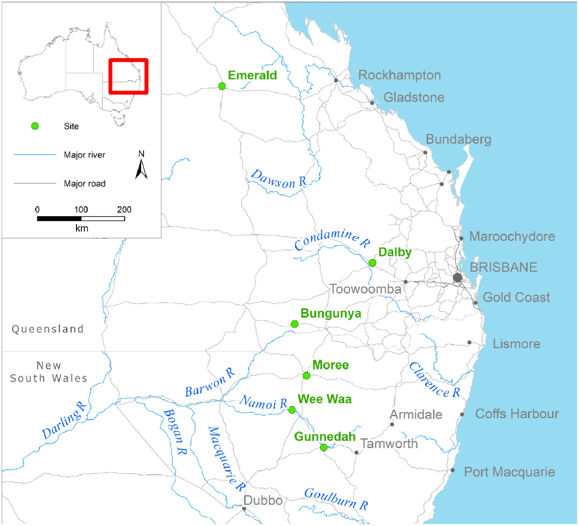
The simulated yields and historical price were combined through copula methods to simulate the economic prospects of rainfed cotton at six locations across NSW and Qld (Fig. 1). In simulation studies where more than one variable is considered, it is important to consider both their distributions and the possibly non-linear dependency between these variables (Wall 1997). Although the Pearson correlation coefficient and multivariate normal distributions are commonly used, there are limitations in using these methods. In particular, the former assumes linearly dependent relationships between the variables, and the latter assumes that all individual variables follow the normal distribution. In reality, the relationship between variables may be non-linear or asymmetric and may exhibit other complicated dependency structures. Also, the individual probability distributions are often asymmetric, skewed or non-normal, and are not the same across all variables. The copula method, which stems from Sklar’s theorem (Sklar 1959), is a flexible tool that can handle all of the aforementioned scenarios (Nelsen 2006; Charpentier and Segers 2007). Copula-based methods have been widely used in finance (Genest et al. 2009) and have made their way into agricultural settings more recently (Hardaker et al. 2015). For example, Nguyen-Huy et al. (2018) used copula methods to obtain the conditional value-at-risk for a wheat-farming portfolio, and Ji et al. (2018) modelled the time-varying dependence structure between energy and agricultural commodity markets through copulas (see Methods: Technical note on copula for more details).
Six rainfed cotton sites in eastern Australia: Emerald, Dalby and Bungunya (near Goondiwindi) in Queensland, and Moree, Wee Waa and Gunnedah in New South Wales (NSW). Source: city and border data spatial from 2019 Esri Data & Maps.
These probabilistic yields and GM results were investigated under different combinations of management options (sowing date and row configuration) under location-specific ranges of weather conditions and prices, and three starting plant-available water (PAW) levels.
Unlike previous studies, this work adds an additional layer of variability in price of cotton and costs associated with production (urea in particular), which can help with identifying those practices that are most robust when price is still an unknown. Given appropriate historical data on weather, costs and prices, this new approach can be applied to cotton and other crops in many parts of the world, assuming that the crop growth can be adequately modelled in software such as OZCOT for cotton (Hearn 1994), AquaCrop (Vanuytrecht et al. 2014) or APSIM (Holzworth et al. 2014).
This study provides: (1) an overview of the simulated yields in the six regions based on long historic, location specific, weather sequences; (2) statistical effects based on the interactions of these conditions (location and starting PAW levels) and agronomic choices; and (3) the combined economic impacts of these practices associated with variability in yield, cost and price, that is, the magnitudes and frequencies of positive and negative GMs achieved through recent history. Depending on the season, the farmer can adjust the sowing date and planting-row configuration to best match the conditions at hand. Historical weather records allow the simulation of distributions of cotton lint yields per hectare, given starting soil PAW (100%, 50% or 30%) for each combination of sowing date and row configuration that the farmer might choose. When combined with yield, the price and cost variations can be used to determine the distributions of GMs per hectare.
Methods
Sites
Six typical rainfed cotton production sites in Australia, encompassing a range of climatic conditions, were selected for analysis (Table 1, Fig. 1). Rainfall and temperature patched-point data from 1945 to 2020 (76 years) for these sites were obtained from SILO climate data systems (Jeffrey et al. 2001). These sites are semi-arid with summer-dominant rainfall, receiving an average of 295–393 mm during the cotton growing season (October–February). Across these sites and through the cotton growing season, the average minimum and maximum temperature ranges were 16.0–20.0°C and 30.3–33.5°C, respectively. The soils across the sites (Table 1) are predominantly Vertosols (SOILpak 1998) according to the Australian Soil Classification system (Isbell 2016), with varied PAW holding capacity (PAWC; see Dalgliesh et al. 2016) of 166–287 mm, to a total soil depth of 1.2 m.
| Location | Latitude and longitude | Soil type | PAWC (mm) | Rainfall (mm) | Oct.–Feb. temperature (°C) | |||
|---|---|---|---|---|---|---|---|---|
| Annual | Oct.–Feb. | Max. | Min. | |||||
| Emerald (Qld) | 23°30′0″S, 148°9′0″E | Vertosol | 287 | 618 (36%) | 393 (40%) | 33.5 (3.27%) | 20.0 (3.31%) | |
| Dalby (Qld) | 27°9′40″S, 151°15′47″E | Vertosol | 285 | 626 (25%) | 372 (35%) | 30.6 (3.83%) | 16.6 (3.89%) | |
| Bungunya (Qld) | 28°25′41″S, 149°39′11″E | Sodosol | 166 | 538 (28%) | 295 (42%) | 32.4 (3.91%) | 18.1 (4.35%) | |
| Moree (NSW) | 29°30′0″S, 149°54′0″E | Vertosol | 214 | 593 (28%) | 327 (42%) | 31.5 (4.27%) | 17.2 (5.52) | |
| Wee Waa (NSW) | 30°12′29″S, 149°35′49″E | Vertosol | 251 | 601 (29%) | 328 (42%) | 31.8 (1.30%) | 16.8 (5.31%) | |
| Gunnedah (NSW) | 30°59′2″S, 150°15′14″E | Vertosol | 207 | 648 (26%) | 356 (37%) | 30.3 (4.25%) | 16.0 (5.43%) | |
Details of agronomic management of cotton used in the simulation are provided below in Simulation treatment. Coefficient of variation (%) in parentheses.
Cotton biophysical modelling
The central component of the OZCOT model is the fruit production and survival subroutine (Hearn and Da Roza 1985). The rates of fruit production, fruit shedding and growth of the organs are governed by carbon supply. Carbon supply for a given day is estimated from intercepted light and crop level photosynthetic rate with respiration deducted. Light interception is estimated, and leaf area generated using an empirical correlation between fruiting site production and leaf area. The leaf expansion rate, photosynthesis and fruiting are modulated by the water supply and nitrogen. The water balance uses a simple moisture extraction routine based on increasing supply with increasing depth of extraction over time (Ritchie 1972). Modifications to the OZCOT model to simulate rainfed skip cotton production systems are described in Milroy et al. (2004). The OZCOT model has been independently validated against field measurements (Carberry and Bange 1998; Milroy et al. 2004; Bange et al. 2005; Richards et al. 2008; Conaty et al. 2018; Darbyshire et al. 2020) for both rainfed and irrigated cotton crops (including commercial crops), and cotton simulations have been tested, and were found to be representative, at several sites, including those chosen for investigation in this study (Roth 2010; Roth et al. 2013; Yang et al. 2014; Williams et al. 2015; Luo et al. 2017; Anwar et al. 2020; Darbyshire et al. 2020; CRDC and CottonInfo 2022). In addition, OZCOT is the same cotton model used in the APSIM crop simulation platform (Holzworth et al. 2014), which has been shown to represent growth and yield processes of cotton accurately under various water conditions (Shukr et al. 2021).
Simulation experiment
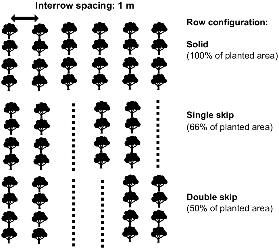
In order to establish the OZCOT model input data, a factorial simulation setup was developed. Representative data for soil parameters, including PAWC at 150–180 cm soil depth in increments of 10–15 cm for each site, were obtained from the APSoil database (Dalgliesh et al. 2009). The factorial design comprised six rainfed cotton growing sites, four sowing dates (30 September, 15 October, 30 October, 15 November), three starting soil water conditions (30% PAW as low, 50% PAW as medium, 100% PAW as high), and three planting-row configurations (solid, single skip, double skip) (Fig. 2), resulting in 36 combinations at each site. Cotton is grown on rows spaced 1 m apart. Solid planting is where seeds are sown in every row (100% of area planted), ‘single skip is where every third row is not planted (66% of area planted), and double skip is where every third and fourth row is not planted (50% area planted). The reduced planting density from using skip rows is used to improve penetration of both sunlight and chemical sprays, and increase access to inter-row soil water by plant roots (where rainfall is expected to be limiting) (Bange et al. 2005). For each factorial combination, the OZCOT model was run using 76 years (1945–2020) of historical weather data (Jeffrey et al. 2001). The model was reset each year at 1 week before the sowing date. By implementing this approach, the yield response for each year was restricted to in-crop season conditions only, and carry-over effects from soil water and nutrient conditions from previous seasons were excluded. Starting soil nitrogen (N) was set at 150 kg/ha. Based on current on-farm practice, N fertiliser (50 kg N/ha) was ‘applied’ as urea at planting. A high-yielding modern cultivar with mid to late maturity and the high fruit retention associated with transgenic cultivars with high levels of insect and pest protection was used in this simulation study.
Statistical analyses
A regression analysis was performed to identify the key factors that affect the yield outcomes. The simulated yields from OZCOT were considered as the response variable, and the agronomic practices (sowing date, row configuration and starting PAW) and location (site) were treated as fixed effects in the model. Interactions between the explanatory variables, except site, were allowed up to the third order. The combination of Emerald (site), 30 September (sowing date), solid (row configuration) and 30% (starting PAW) was chosen as the reference level against which the other factor combinations were compared. Different levels within each factor were compared using Tukey’s post hoc approach at the P = 0.05 family-wise error rate. Regression analysis was conducted using R (R Core Team 2020). Several R packages were used during data preparation, analysis and visualisation, including: tidyverse (Wickham et al. 2019) and ggplot2 (Wickham 2016).
Gross margin budgets
Gross margins were calculated as ‘enterprise’ income (i.e. cotton crop sales) less variable costs (Malcolm et al. 2005). Incomes were derived by multiplying cotton bale prices by simulated crop yields. Probabilistic GM budgets for all six sites were generated using a multivariate distribution estimated from the historical price, simulated yield and cost of applied urea. The data inputs for the copula analysis comprised more than seven decades (76 years) of yields (no. of bales/ha) from 1945 to 2020, and 35 years of varying annual average cotton bale prices (AU$/bale, where 1 bale = 227 kg lint) and urea prices ($/kg) from 1984–85 to 2018–19 (ABARES 2019). The univariate distribution for each of these three key input variables was chosen using the Akaike information criterion (AIC), and the parameters were estimated using the maximum likelihood method (Hardaker et al. 2015; Palisade Corporation 2021). The two price and cost variables were deflated to the base year of 2018–19. All other costs for solid, single skip and double skip planting configuration were taken from the GM budget estimates for the financial year 2018–19 reported in CottonInfo (2018); see Table 2 for further details. A proportional cost was allocated to the solid row configuration. Cotton price adjustments for fibre quality discounts were made for the solid ($135/bale) and single skip ($25/bale) row configurations (Bange et al. 2005).
| Real Price Australian gin-gate return (AU$/bale) (distributions bounded by copula)A | Simulated from fitted distributions and copula (refer to Figs 4, 5). The two variables of price and yield multiplied together gave revenue for each site–tactical decision and accounted for price and production variability for each location. | |||
| Yield (no. of bales/ha): OZCOT simulated data from 1945 to 2020 (distributions bounded by copula)B | ||||
| Variable costs by operationC | Solid | Single skip | Double skip | |
|---|---|---|---|---|
| Fertiliser applied: nutrition urea (50 kg N) (Real Price ($/kg) × fertiliser applied (50 kg))D |  Price simulated according to a uniform distribution bounded between $0.546 and $1.124/kg, and is further multiped by 50 kg urea applied/haE Price simulated according to a uniform distribution bounded between $0.546 and $1.124/kg, and is further multiped by 50 kg urea applied/haE | |||
| Fallow management ($/ha) | 73 | 73 | 73 | |
| Planting and in-crop farming ($/ha) | 110 | 87 | 69 | |
| Crop protection, application and licence fee ($/ha) | 432 | 395 | 361 | |
| Defoliation ($/ha) | 196 | 141 | 102 | |
| Picking (cartage + cartage and ginning costs/rows excluded) ($/ha) | 366 | 332 | 301 | |
| Farming: post-crop ($/ha) | 47 | 47 | 47 | |
| Insurance ($/ha) | 101 | 90 | 80 | |
| Fibre length discount ($/ha) | 135 | 25 | 0 | |
| Total variable cost (actual cost varies owing to randomness of the price of urea) ($/ha) | 1459 | 1190 | 1032 | |
Source: modified from Powell et al. (2020)
AABARES Real Price Australian gin-gate return (AU$/bale): data taken from 1984–85 to 2018−19. 2018−19 was used as base year to convert nominal prices to real. Price combined ABARES lint yield Qld and NSW (t/ha) for the same period using copula functions to capture the dependency structures among these two variables.
BLint was converted to no. bales/ha. We assumed that the cotton farm has a ‘gin for seed’ contract; hence, no dollar value was allocated to cotton seeds. Ginning and cartage costs were not considered because these are almost the same as the proceeds from the sale of cotton seed and so are offset. We also assumed that lint quality was uniform and that no dockages (discounts) were made for quality.
CVariable cost of solid planting was based on the proportional cost of of single skip to double skip planting. For example, the cost of single-skip planting and in-crop farming was 1.27 times the double skip. Therefore $87 × 1.27 = $110.
DABARES Real Urea Price ($/kg): data taken from 1984−85 to 2018−19. 2018−19 was used as base year to convert nominal price to real. 2013−14 onwards missing data sourced from Index Mundi. Nutrition replaced in Powell et al. (2020) GM budget.
ETo view the above figure in colour, please see the online version of this journal.
After fitting the individual distributions of cotton price and yield, the joint distribution in the form of a copula was also estimated, which was then used to simulate both yields and prices with their dependencies considered. For each risk-management scenario, the model was run over 10 000 iterations of Monte Carlo simulation. The GMs calculated from these iterations were used to derive the distributions of the GMs for further comparisons. A similar approach was adopted in Godfrey et al. (2021, 2022). All computational steps to derive GMs were performed using @Risk 8.2 software (Palisade Corporation 2021).
Technical note on copula
In this study, we treated yield and price as two correlated random variables. Simulation of jointly distributed variables was facilitated by using the copula approach. Such an approach is relatively new in agricultural studies; therefore, a brief overview is provided here. In order to capture the co-movement of two variables in simulations, the bivariate distribution needs to be estimated. Sklar’s theorem states that there exist functions called copulas such that all bivariate distributions can be represented as a copula of their univariate distributions (Shemyakin and Kniazev 2017). For example, one could combine two variables, where one follows the uniform distribution and the other follows the normal distribution, by using a copula. The allowance of separate estimations for the marginal and joint distributions is considered a main advantage of using copulas (Genest and Favre 2007; Bouri et al. 2018).
Different types of copula models have been derived. Popular ones include the Gaussian, Student’s t, Gumbel, Clayton and Frank copulas (Patton 2012). Among these, the Frank copula, which will be presented in the Results, admits the form (Hove et al. 2017):
where θ ≠ 0 is a parameter to be estimated from the observed pair of variables u and v. Hove et al. (2017) showed that θ is related to the rank correlation between u and v. Practically, analysts must rely on software to estimate the copula parameter(s) and select the copula type that best fit the data. To improve the flexibility, it is common to consider ‘rotated’ copulas where one axis is rotated by 180° to allow negative correlations or even more sophisticated dependency structures such as asymmetric tail dependence (Wali et al. 2018; Mensah and Adam 2020). Readers are referred to Nelsen (2006) and Hardaker et al. (2015) for more technical details regarding the copula approach. Some practical implementation details using @Risk can be found in Godfrey et al. (2022).
Results
From the farmer’s viewpoint, from the start, the following things are known for certain: the farm’s location, and accompanying soil and historical climate information. Another piece of information is important in forming a strategy for sowing rainfed cotton at a particular location: starting PAW at the sowing time. Given this information, it is then possible, using the results described below, to select one of the 12 combinations of management practices (sowing date and row configuration) that is likely to perform well on average (based on GMs per hectare) given the associated variability in yield, cost and price. At most locations, a wide variation in projected outcomes from the different combinations of management practices is apparent. Each location is unique in responses owing to differences in latitude, altitude, rainfall, temperature and soil conditions.
Cotton yields
All interaction effects between explanatory variables were not statistically significant at P = 0.05 and were removed from the final linear model. Table 3 depicts the results of analysis of variance and the estimated coefficients of the final model for cotton yield, and Fig. 3 shows the distributions of yields simulated from OZCOT at two selected locations (see Supplementary materials for other locations), under three starting PAW levels and 12 combinations of managerial practices formed from four sowing times and three row configurations.
| SS | d.f. | F-statistic | P | Coefficient | s.e. | t-value | P-value | ||
|---|---|---|---|---|---|---|---|---|---|
| Intercept | 3.435 | 0.049 | 69.82 | <0.001 | |||||
| Site | 5673 | 5 | 371.18 | <0.001 | |||||
| Emerald | – | – | – | – | |||||
| Dalby | 0.185 | 0.047 | 3.913 | <0.001 | |||||
| Bungunya | −1.275 | 0.047 | −26.98 | <0.001 | |||||
| Moree | −1.310 | 0.047 | −27.72 | <0.001 | |||||
| Wee Waa | −0.503 | 0.047 | −10.64 | <0.001 | |||||
| Gunnedah | −0.974 | 0.047 | −20.62 | <0.001 | |||||
| Sowing time | 50 | 3 | 5.4575 | 0.001 | |||||
| 30 Sept. (a) | – | – | – | – | |||||
| 15 Oct. (b) | 0.116 | 0.039 | 3.009 | 0.003 | |||||
| 30 Oct. (b) | 0.148 | 0.039 | 3.835 | 0.000 | |||||
| 15 Nov. (ab) | 0.097 | 0.039 | 2.511 | 0.012 | |||||
| Row configuration | 94 | 2 | 15.372 | <0.001 | |||||
| Solid (c) | – | – | – | – | |||||
| Single skip (b) | −0.070 | 0.033 | −2.100 | 0.036 | |||||
| Double skip (a) | −0.183 | 0.033 | −5.494 | <0.001 | |||||
| Starting PAW | 4798 | 2 | 784.91 | <0.001 | |||||
| Low (a) | – | – | – | – | |||||
| Medium (b) | 0.492 | 0.033 | 14.71 | <0.001 | |||||
| High (c) | 1.311 | 0.033 | 39.22 | <0.001 | |||||
| Residual SS = 50 139 on 16 403 d.f. |
Within sowing time, row configuration or starting PAW, levels followed by the same letter (in parentheses) are not significantly different based on Tukey’s post hoc pairwise comparisons using the 5% family-wise error rate. The reference levels for site, sowing date, row configuration and starting PAW are Emerald, 30 September, solid and 30%, respectively.
SS, sum of squares; d.f., degrees of freedom; s.e., standard error.
Two boxplot distributions (top, Dalby; bottom, Moree) shown for each combination of PAW, row configuration and sowing date. Left (blue) boxplot represents rainfed cotton lint yields relative to the overall mean (dashed blue line, 3.40 bales/ha) across all six sites and treatments. Right (red) boxplot represents gross margins (GM) relative to zero (solid red line). In each boxplot, the line in the middle of the box represents the median value for the data, the upper edge of the box the 75th percentile, and the lower edge the 25th percentile. The whiskers correspond to 1.5 times the interquartile range (difference between 75th and 25th percentiles) or to the most extreme observed value, whichever is smallest. Crosses above or below the whiskers represent individual values outside of this range.
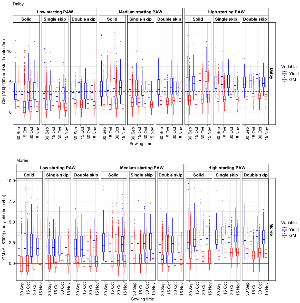
Considering all 216 combinations, the average annual cotton yield was 3.40 bales/ha. Median yield ranged from 1.39 to 5.46 bales/ha, standard deviation from 1.08 to 2.54 bales/ha, and interquartile range from 1.35 to 3.68 bales/ha. From Fig. 3 and Table 3, large site-to-site variations can be observed (P < 0.001). On average, Moree had the lowest yields, and Dalby had the highest yields, with an average difference of 1.50 bales/ha.
Each individual factor significantly impacted the yield of cotton (all P < 0.001, Table 3). The third sowing date (30 October) tended to provide the highest yield, followed by the second sowing date (15 October) and then the latest one (15 November). The earliest sowing time (30 September) led to a significantly lower yield than both 15 October and 30 October (Table 3). Compared with the earliest sowing time, sowing on 15 October and 30 October provided an extra yield of 0.12 and 0.15 bales/ha, on average, respectively (Table 3).
All three row configurations provided significantly different effects on yields (Table 3). Solid row configuration was estimated to provide extra yield of 0.07 and 0.18 bales/ha over single and double skip, respectively (Table 3).
Likewise, the three levels of starting PAW provided significantly different effects on yields (Table 3). High and medium starting PAW led to extra yield of 1.31 and 0.49 bales/ha, respectively, over low starting PAW (Table 3).
Considering yields alone, these results suggest that the combination of solid row configuration and sowing on 30 October would be the best tactical option, regardless of the level of starting PAW. However, this option may not be the best from the profitability perspective, as illustrated later.
Relationship between yield and prices
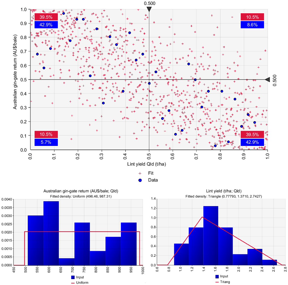
Uniform distributions provided the best fit for the Australian gin-gate return prices for cotton bales recorded in both Qld and NSW, whereas triangular distributions provided the best fit for the lint yields (Figs 4, 5). Regarding the bivariate relationship between Australian gin-gate return prices and lint yields, the Frank copula with the vertical axis flipped (called ‘FrankRX copula’ in @Risk) provided the best fit the data according to the AIC evaluated by the software. The use of the FrankRX copula function suggests that the relationship between Australian gin-gate return price and lint yield was negative and exhibited symmetric dependence in both positive and negative tails (Hove et al. 2017). The estimated parameters (θ = 6.46 and 6.87 in NSW and Qld, respectively) indicate that these two variables were moderately to strongly correlated (Genest 1987; Escarela and Carriere 2003). The rank correlations of the two variables were −0.72 and −0.79 in NSW and Qld, respectively. The red crosses on the top panels of Figs 4 and 5 present the sample simulated values (before transforming back to the original scales) based on the fitted copula. These were used to calculate the GMs as reported in the next part. Because all Australian cotton is sold on the world market, it is bound up in the scenario of low prices when world production and stocks are high, and higher prices when world production and stocks are low.
Top panel: observed (blue circles) and fitted (red crosses) bivariate relationship between Australian gin-gate return in real terms and lint yield from 1984–85 to 2018–19 in Queensland. The fitted data were simulated based on the FrankRX copula that was used to generate the gross margins. The data are presented in a standardised way on a 0–1 scale. The red and blue text boxes show the percentages of the values (of each variable) present in each quadrant of the graph. Bottom panel: observed (blue bars) and fitted (red line) univariate distributions for Australian gin-gate return (left) and lint yield (right) in Queensland used as inputs in fitting the copula.
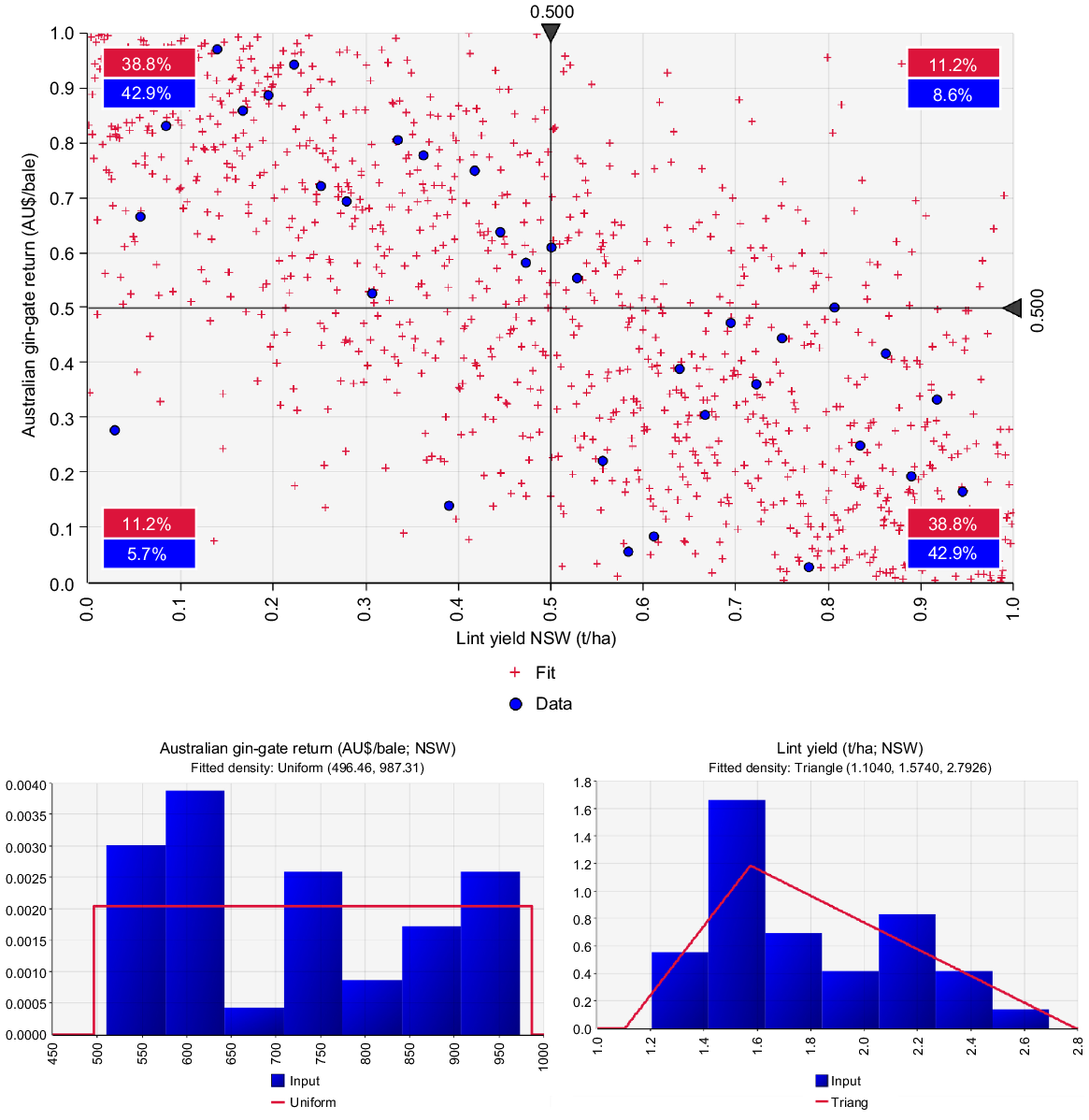
Top panel: observed (blue circles) and fitted (red crosses) bivariate relationship between Australian gin-gate return in real terms and lint yield from 1984–85 to 2018–19 in New South Wales. The fitted data were simulated based on the FrankRX copula that was used to generate the gross margin. Data are presented in a standardised way on a 0–1 scale. The red and blue text boxes show the percentages of the values (of each variable) present in each quadrant of the graph. Bottom panel: observed (blue bars) and fitted (red line) univariate distributions for Australian gin-gate return (left) and lint yield (right) in New South Wales used as inputs in fitting the copula.
Gross margins
The GM distributions for all 36 combinations of factors for Dalby and Moree are given in Fig. 3 alongside the yields. Supplementary Fig. S1 shows the distributions for the other four locations. Across all 216 combinations of factors, the average GM was $1118/ha. Median GM ranged from −$310/ha (i.e. a loss) to $2659/ha, standard deviations from $610/ha to $1674/ha, and interquartile ranges from $763/ha to $2636/ha.
From Figs 3 and S1, it can be seen that higher levels of yield often led to higher GMs. Although there was a negative relationship between price and yield, these were multiplied together to form the revenue. A higher GM is possible when the increment in yield could compensate the decrement in price. Nevertheless, the increase in variabilities in GM compared with the yields is noteworthy, and is expected because these include variabilities in price and cost. Across all 216 combinations, the median coefficient of variation (CV%) for GM was 94% whereas that for yield was 54%. There was also extra variability in GM at higher yield combinations, which may be a result of the local price being negatively correlated with local yield. Thus, a positive yield may not mean a worthwhile investment. In fact, considering yield alone could seriously underestimate the risk involved. At lower yields, these effects will result in less overall variability in GM.
From Figs 3 and S1, large variations across the locations were observed. The most beneficial (depending on different criteria) combinations of starting PAW, row configuration and sowing date at each site are shown in Table 4. More detailed summary statistics can be found in Table S1. Although the combination of solid row configuration and sowing on 30 October tended to provide the highest yield, such a combination is never projected to provide the highest mean or median GM across all sites and starting PAW (Table 4). In fact, Table 4 also shows that single and double skip were found to provide a higher mean or median GM than solid row configuration in many scenarios. In most cases, double skip was found to be a more resilient strategy in terms of minimising the ‘lower tail’ risk using either the fifth percentile or the percentage of negative GMs as a measure.
| High starting PAW | Medium starting PAW | Low starting PAW | ||||||||
|---|---|---|---|---|---|---|---|---|---|---|
| Site | Row configuration | Sowing date | Mean ($’000/ha) | Row configuration | Sowing date | Mean ($’000/ha) | Row configuration | Sowing date | Mean ($’000/ha) | |
| Highest mean GMs | ||||||||||
| Emerald | Single skip | 15 Oct. | 2.44 | Single skip | 15 Nov. | 1.69 | Double skip | 15 Nov. | 1.26 | |
| Dalby | Double skip | 30 Oct. | 2.68 | Double skip | 30 Sept. | 1.91 | Double skip | 30 Sept. | 1.42 | |
| Bungunya | Double skip | 15 Nov. | 1.74 | Double skip | 30 Oct. | 0.85 | Solid | 15 Nov. | 0.40 | |
| Moree | Solid | 30 Sept. | 1.48 | Single skip | 30 Oct. | 0.78 | Single skip | 15 Nov. | 0.49 | |
| Wee Waa | Single skip | 30 Oct. | 2.13 | Single skip | 30 Sept. | 1.27 | Single skip | 30 Sept. | 0.92 | |
| Gunnedah | Double skip | 15 Oct. | 1.59 | Double skip | 30 Sept. | 1.23 | Double skip | 30 Sept. | 1.14 | |
| High starting PAW | Medium starting PAW | Low starting PAW | ||||||||
|---|---|---|---|---|---|---|---|---|---|---|
| Site | Row configuration | Sowing date | Median ($’000/ha) | Row configuration | Sowing date | Median ($’000/ha) | Row configuration | Sowing date | Median ($’000/ha) | |
| Highest median GMs | ||||||||||
| Emerald | Single skip | 15 Oct. | 2.40 | Single skip | 15 Nov. | 1.72 | Double skip | 15 Nov. | 1.24 | |
| Dalby | Double skip | 30 Oct. | 2.66 | Double skip | 30 Oct. | 1.90 | Double skip | 30 Oct. | 1.42 | |
| Bungunya | Double skip | 15 Nov. | 1.75 | Double skip | 30 Oct. | 0.79 | Solid | 15 Nov. | 0.32 | |
| Moree | Solid | 30 Sept. | 1.37 | Single skip | 30 Oct. | 0.72 | Single skip | 15 Nov. | 0.41 | |
| Wee Waa | Single skip | 30 Oct. | 2.04 | Single skip | 30 Sept. | 1.15 | Single skip | 30 Sept. | 0.82 | |
| Gunnedah | Double skip | 15 Oct. | 1.64 | Double skip | 30 Sept. | 1.23 | Double skip | 30 Sept. | 1.25 | |
| High starting PAW | Medium starting PAW | Low starting PAW | ||||||||
|---|---|---|---|---|---|---|---|---|---|---|
| Site | Row configuration | Sowing date | 5th percentile ($’000/ha) | Row configuration | Sowing date | 5th percentile ($’000/ha) | Row configuration | Sowing date | 5th percentile ($’000/ha) | |
| Highest fifth-percentile GMs | ||||||||||
| Emerald | Single skip | 15 Oct. | 1.35 | Double skip | 30 Oct. | 0.03 | Double skip | 15 Nov. | −0.23 | |
| Dalby | Double skip | 30 Oct. | 1.59 | Double skip | 15 Nov. | 0.55 | Double skip | 15 Nov. | −0.09 | |
| Bungunya | Double skip | 15 Nov. | 0.66 | Double skip | 30 Sept. | −0.42 | Double skip | 30 Sept. | −0.80 | |
| Moree | Single skip | 15 Nov. | 0.34 | Single skip | 30 Sept. | −0.59 | Single skip | 15 Nov. | −0.78 | |
| Wee Waa | Double skip | 15 Oct. | 0.84 | Double skip | 30 Sept. | −0.32 | Double skip | 30 Oct. | −0.71 | |
| Gunnedah | Double skip | 15 Oct. | 0.43 | Double skip | 30 Oct. | −0.21 | Double skip | 30 Oct. | −0.40 | |
| High starting PAW | Medium starting PAW | Low starting PAW | ||||||||
|---|---|---|---|---|---|---|---|---|---|---|
| Site | Row configuration | Sowing date | Percentage | Row configuration | Sowing date | Percentage | Row configuration | Sowing date | Percentage | |
| Lowest percentage of negative GMsA | ||||||||||
| Emerald | Single skip | 15 Oct. | 0.00 | Double skip | 30 Oct. | 4.70 | Double skip | 15 Nov. | 8.30 | |
| Dalby | Double skip | 30 Oct. | 0.00 | Double skip | 15 Nov. | 0.10 | Double skip | 15 Nov. | 7.10 | |
| Bungunya | Double skip | 15 Nov. | 0.00 | Double skip | 30 Oct. | 16.8 | Double skip | 15 Oct. | 38.7 | |
| Moree | Single skip | 15 Nov. | 0.70 | Single skip | 30 Oct. | 21.5 | Single skip | 15 Nov. | 33.2 | |
| Wee Waa | Double skip | 15 Oct. | 0.00 | Double skip | 30 Sept. | 11.0 | Single skip | 30 Sept. | 26.3 | |
| Gunnedah | Single skip | 15 Nov. | 1.30 | Double skip | 30 Oct. | 7.90 | Double skip | 30 Oct. | 14.0 | |
AWhen multiple combinations have the same minimum, the one that gives the highest mean GM is reported.
At all locations, it is no surprise that the probability of obtaining positive GMs was the lowest with low starting PAW, and highest with high PAW (Table 4). At Bungunya and Moree, when the starting PAW was low, negative GMs were projected in at least one-third of instances, even with the best management practice. At the Emerald and Dalby, there were still good chances of getting a positive GM even with a low starting PAW, most likely associated with higher summer-dominant rainfall. Below we demonstrate how the distributions of GM provided in Fig. 3 and the statistics in Table 4 can be used jointly to obtain some site-specific features.
At Dalby, Qld, double-skip row configuration and sowing on 30 October tended to give the highest median GM with all three starting PAW levels (Fig. 3). When the starting PAW was high, such a strategy never resulted in a negative GM based on simulation results. Of course, this does not apply to standing flood conditions, which destroy crops however they are spaced. When the starting PAW is either medium or low, double-skip row configuration and sowing on 15 November tended to be least risky.
At Moree, NSW, when the starting PAW was low, the chance of having a positive GM was sometimes less than half, especially when solid row configuration was used (Fig. 3). Single-skip row configuration and late sowing (30 October or 15 November) gave the highest chance of having positive GMs under all three levels of starting PAW (Table 4). These combinations also tended to result in the highest mean and median GMs under low and medium starting PAW (Fig. 3, Table 4). However, under high starting PAW, solid row configuration and sowing on 30 September was the best option for achieving the highest mean or median GM.
Discussion
Farmers know the specific characteristic soils and historical climate variabilities of their location. Farmers can also measure or judge the PAW status of a field before sowing. Given these conditions, the farmer may then use the data published here to choose a combination of sowing date and row configuration (solid, single skip, or double skip) in order to maximise the probability of growing a profitable crop, as summarised in Figs 3 and S1, and Tables 4 and S1.
As with other investors, different farmers have different attitudes towards risk (Iyer et al. 2020). Some may prefer taking a higher risk if the potential profit is higher, whereas others prefer a less risky option. Table S1 provides various summary statistics of the GM distributions, which can be used to conduct further analyses based on some desired criteria such as highest mean GM or lowest chance of having a negative GM.
In this study the results for cotton crop yield were quite different from the GMs in terms of means, medians and variability. This is because GM can be negative while yields are always non-negative, meaning that a positive yield may not mean a worthwhile investment. Hence, it is important to consider rainfed cotton crops from the perspective of GM. To our knowledge, data that shed light on this topic for rainfed cotton based on distributions coming from historical price and yield data and simulated based on their dependencies generated by copula have not been previously published.
Given the inclusion of considerations of prices as well as yield, GMs are generally more variable than yield. Our results starkly contrast the likely outcomes of the two combined management factors decided by farmers (row configuration and sowing date) when given three starting PAW scenarios in the six farming areas, taking into account the known historical variations in weather and in cotton and input price variations over the long term (76 years for weather and 35 years for urea costs and cotton prices). The use of this information may help to shape selection of management options when there are different degrees of uncertainty involved. In this study, it was assumed that the three variables (urea costs, cotton prices and yields) were effectively unknown by the grower at the start of the cropping season. Further understanding is needed to assess how this information influences decision-making leading into a cotton season where choices of sowing time and configuration are available to the farmer. It may be that these analyses exclude management choices for a grower that are not options in any scenario. For example, a scenario such as a dry year with less than 10% PAW, which leaves rainfed cotton prospects so poorly that sowing cannot be recommended, is not covered in the present study. Therefore, as more information is known (such as cost and price/or price range), analyses can focus on a smaller set of management options allowing for simplicity in interpretation (fewer scenarios) plus more in-depth analysis of those scenarios that are important. Obviously, analysis should then generate GM distributions with the inclusion of known information. How these analyses are used for decision-making in light of access to information sources will be a subject for further research. Further research will also seek to understand how these insights can be used to add value to the decision-making of growers, in contrast to more traditional approaches of assessing risk using predefined but limited combinations of price, cost and yield.
Owing to technological advances and economies of scale, real cotton prices tend to be decreasing over time. It could be argued that the use of price data from 30 years ago might have inflated the overall expected price used in the analysis, because farmers today are unlikely to receive the high prices from 20 or 30 years ago. However, our propose is not to prepare management decisions for farmers in 2023 or 2024, but to illustrate the sorts of variations that they face in the long term. For this purpose, the wider the variations, the clearer the big picture. The past 30 years of data have included many possibilities of price fluctuations including the Millennium Drought. Recent unexpected events, including the COVID-19 pandemic and the Ukraine-Russian war have revealed how vulnerable the supply chain is, and how volatile the prices of energy and commodities can be. Therefore, we argue that it is important to include a wide range of prices in the model. Future research may seek to investigate the relationship between the crop yields at local sites and the total industrial supply, with the area planted considered. This may give an indication of how local cotton prices are affected by the overall Australian, or even international, cotton prices, which may better reflect the profitability at farm level.
Throughout the simulation study, it was assumed that the total amount of N was not crop limiting (150 kg/ha starting, plus 50 kg/ha applied) for any of the locations. A direction for future research may be to start with different soil N levels and seek the optimal strategies for fertiliser applications.
Of course, our analysis does not predict how these scenarios might have, or will be, changed by climate change. It is possible that the approaches used here are already capturing these climate-change effects and producing appropriate outcomes reflecting changes over time. This topic will be also the subject of further research.
Conclusion
Our probabilistic simulation model incorporated yield, price and cost uncertainty explicitly based on the distributions and historical relationship of these input variables in order to compare rainfed cotton yields and GMs within and across six locations to assist in business performance of these regions. The method used here is coming into practice in business and can be applied to other agricultural contexts. Long-term seasonal weather forecasting will likely continue to improve and add value to these analyses. Results and techniques presented in this paper may assist growers of rainfed cotton to manage risk in their enterprises. The challenge remains as to how to deliver this information to growers effectively.
Acknowledgements
We thank Deanna Duffy, Spatial Analysis Officer, Spatial Analysis Unit (SPAN), Charles Sturt University, Wagga Wagga, for producing the map of rainfed cotton regions. We also thank Janine Powell, Economist and Partner AgEcon, Narrabri, NSW, for replying to our questions related to the costs of rainfed cotton production. We are grateful for the insights offered in the comments from anonymous reviewers and editors.
References
Anwar MR, Wang B, Liu DL, Waters C (2020) Late planting has great potential to mitigate the effects of future climate change on Australian rain-fed cotton. Science of The Total Environment 714, 136806.
| Crossref | Google Scholar |
Archontoulis SV, Miguez FE (2015) Nonlinear regression models and applications in agricultural research. Agronomy Journal 107, 786-798.
| Crossref | Google Scholar |
Ashton D (2019) Cotton farms in the Murray–Darling Basin. Australian Bureau of Agricultural and Resource Economics and Sciences, Canberra, ACT, Australia. Available at https://www.awe.gov.au/abares/research-topics/surveys/irrigation/cotton#cotton--production-in-the-murraydarling-basin [Accessed 20 April 2022]
Bange MP, Carberry PS, Marshall J, Milroy SP (2005) Row configuration as a tool for managing rain-fed cotton systems: review and simulation analysis. Australian Journal of Experimental Agriculture 45, 65-77.
| Crossref | Google Scholar |
Bange MP, Constable GA, Johnston DB, Kelly D (2010a) A method to estimate the effects of temperature on cotton micronaire. The Journal of Cotton Science 14, 164-172.
| Google Scholar |
Bouri E, Gupta R, Lau CKM, Roubaud D, Wang S (2018) Bitcoin and global financial stress: a copula-based approach to dependence and causality in the quantiles. The Quarterly Review of Economics and Finance 69, 297-307.
| Crossref | Google Scholar |
Charpentier A, Segers J (2007) Lower tail dependence for Archimedean copulas: characterizations and pitfalls. Insurance: Mathematics and Economics 40, 525-532.
| Crossref | Google Scholar |
Conaty WC, Johnston DB, Thompson AJE, Liu S, Stiller WN, Constable GA (2018) Use of a managed stress environment in breeding cotton for a variable rainfall environment. Field Crops Research 221, 265-276.
| Crossref | Google Scholar |
Cotton Incorporated (2022) Why irrigate cotton? Available at https://www.cottoninc.com/cotton-production/ag-resources/irrigation-management/why-irrigate-cotton/ [Accessed 20 April 2022]
CRDC and CottonInfo (2022) Australian cotton production manual 2022. Cotton Research and Development Corporation, Narrabri, NSW, Australia. Available at https://www.cottoninfo.com.au/sites/default/files/documents/2022%20ACPM%20final.pdf [Accessed 28 March 2023]
Dalgliesh NP, Foale MA, McCown RL (2009) Re-inventing model-based decision support with Australian dryland farmers. 2. Pragmatic provision of soil information for paddock-specific simulation and farmer decision making. Crop & Pasture Science 60, 1031-1043.
| Crossref | Google Scholar |
Dalgliesh NP, Hochman Z, Huth N, Holzworth D (2016) Field protocol to APSoil characterisations. Version 4. CSIRO, Australia. Available at https://publications.csiro.au/rpr/download?pid=csiro:EP166550&dsid=DS4 [Accessed 28 March 2023]
Darbyshire R, Crean J, Cashen M, Anwar MR, Broadfoot KM, Simpson M, Cobon DH, Pudmenzky C, Kouadio L, Kodur S (2020) Insights into the value of seasonal climate forecasts to agriculture. Australian Journal of Agricultural and Resource Economics 64, 1034-1058.
| Crossref | Google Scholar |
Escarela G, Carriere JF (2003) Fitting competing risks with an assumed copula. Statistical Methods in Medical Research 12, 333-349.
| Crossref | Google Scholar |
Genest C (1987) Frank’s family of bivariate distributions. Biometrika 74, 549-555.
| Crossref | Google Scholar |
Genest C, Favre A-C (2007) Everything you always wanted to know about copula modeling but were afraid to ask. Journal of Hydrologic Engineering 12, 347-368.
| Crossref | Google Scholar |
Genest C, Gendron M, Bourdeau-Brien M (2009) The advent of copulas in finance. The European Journal of Finance 15, 609-618.
| Crossref | Google Scholar |
Godfrey SS, Nordblom T, Ip RHL, Robertson S, Hutchings T, Behrendt K (2021) Drought shocks and gearing impacts on the profitability of sheep farming. Agriculture 11, 366.
| Crossref | Google Scholar |
Godfrey SS, Ip RHL, Nordblom TL (2022) Risk analysis of Australia’s Victorian dairy farms using multivariate copulae. Journal of Agricultural and Applied Economics 54, 72-92.
| Crossref | Google Scholar |
Hearn AB (1994) OZCOT: a simulation model for cotton crop management. Agricultural Systems 44, 257-299.
| Crossref | Google Scholar |
Hearn AB, Da Roza GD (1985) A simple model for crop management applications for cotton (Gossypium hirsutum L.). Field Crops Research 12, 49-69.
| Crossref | Google Scholar |
Holzworth DP, Huth NI, deVoil PG, Zurcher EJ, Herrmann NI, McLean G, Chenu K, et al. (2014) APSIM – evolution towards a new generation of agricultural systems simulation. Environmental Modelling & Software 62, 327-350.
| Crossref | Google Scholar |
Hove H, Beichelt F, Kapur PK (2017) Estimation of the frank copula model for dependent competing risks in accelerated life testing. International Journal of System Assurance Engineering and Management 8, 673-682.
| Google Scholar |
ICAC (2022) Cotton this Month. 1 April 2022. International Cotton Advisory Committee, Washington, DC, USA. Available at https://www.icac.org/Content/PublicationsPdf%20Files/9f1e2ebf_03c6_479c_9503_26d4c964d8a7/CTM_2022_04_01.pdf.pdf [Accessed 20 April 2022]
Iyer P, Bozzola M, Hirsch S, Meraner M, Finger R (2020) Measuring farmer risk preferences in Europe: a systematic review. Journal of Agricultural Economics 71, 3-26.
| Crossref | Google Scholar |
Jeffrey SJ, Carter JO, Moodie KB, Beswick AR (2001) Using spatial interpolation to construct a comprehensive archive of Australian climate data. Environmental Modelling & Software 16, 309-330.
| Crossref | Google Scholar |
Ji Q, Bouri E, Roubaud D, Shahzad SJH (2018) Risk spillover between energy and agricultural commodity markets: a dependence-switching CoVaR-copula model. Energy Economics 75, 14-27.
| Crossref | Google Scholar |
Luo Q, Behrendt K, Bange M (2017) Economics and risk of adaptation options in the Australian cotton industry. Agricultural Systems 150, 46-53.
| Crossref | Google Scholar |
Mensah PO, Adam AM (2020) Copula-based assessment of co-movement and tail dependence structure among major trading foreign currencies in Ghana. Risks 8, 55.
| Crossref | Google Scholar |
Milroy SP, Bange MP, Hearn AB (2004) Row configuration in rainfed cotton systems: modification of the OZCOT simulation model. Agricultural Systems 82, 1-16.
| Crossref | Google Scholar |
Nguyen-Huy T, Deo RC, Mushtaq S, An-Vo D-A, Khan S (2018) Modeling the joint influence of multiple synoptic-scale, climate mode indices on Australian wheat yield using a vine copula-based approach. European Journal of Agronomy 98, 65-81.
| Crossref | Google Scholar |
Patton AJ (2012) A review of copula models for economic time series. Journal of Multivariate Analysis 110, 4-18.
| Crossref | Google Scholar |
Porter JR, Semenov MA (2005) Crop responses to climatic variation. Philosophical Transactions of the Royal Society B: Biological Sciences 360, 2021-2035.
| Crossref | Google Scholar |
Portmann F T, Siebert S, Döll P (2010) MIRCA2000 – Global monthly irrigated and rainfed crop areas around the year 2000: a new high-resolution data set for agricultural and hydrological modeling. Global Biogeochemical Cycles 24, GB1011.
| Crossref | Google Scholar |
Richards QD, Bange MP, Johnston SB (2008) HydroLOGIC: an irrigation management system for Australian cotton. Agricultural Systems 98, 40-49.
| Crossref | Google Scholar |
Ritchie JT (1972) Model for predicting evaporation from a row crop with incomplete cover. Water Resources Research 8, 1204-1213.
| Crossref | Google Scholar |
Roth G (2010) Economic, environmental and social sustainability indicators of the Australian cotton industry. Available at https://www.crdc.com.au/sites/default/files/pdf/Economic%2C%20social%20and%20environmental%20indicators%20report.pdf [Accessed 28 March 2023]
Roth G, Harris G, Gillies M, Montgomery J, Wigginton D (2013) Water-use efficiency and productivity trends in Australian irrigated cotton: a review. Crop & Pasture Science 64, 1033-1048.
| Crossref | Google Scholar |
Shukr HH, Pembleton KG, Zull AF, Cockfield GJ (2021) Impacts of effects of deficit irrigation strategy on water use efficiency and yield in cotton under different irrigation systems. Agronomy 11, 231.
| Crossref | Google Scholar |
Turner NC, Hearn AB, Begg JE, Constable GA (1986) Cotton (Gossypium hirsutum L.): physiological and morphological responses to water deficits and their relationship to yield. Field Crops Research 14, 153-170.
| Crossref | Google Scholar |
Vanuytrecht E, Raes D, Steduto P, Hsiao TC, Fereres E, Heng LK, Garcia Vila M, Mejias Moreno P (2014) AquaCrop: FAO’s crop water productivity and yield response model. Environmental Modelling & Software 62, 351-360.
| Crossref | Google Scholar |
Wali B, Greene DL, Khattak AJ, Liu J (2018) Analyzing within garage fuel economy gaps to support vehicle purchasing decisions – a copula-based modeling & forecasting approach. Transportation Research Part D: Transport and Environment 63, 186-208.
| Crossref | Google Scholar |
Wall DM (1997) Distributions and correlations in Monte Carlo simulation. Construction Management and Economics 15, 241-258.
| Crossref | Google Scholar |
Wickham H, Averick M, Bryan J, Chang W, McGowan L, François R, Grolemund G, Hayes A, Henry L, Hester J, Kuhn M, Pedersen T, Miller E, Bache S, Müller K, Ooms J, Robinson D, Seidel D, Spinu V, Takahashi K, Vaughan D, Wilke C, Woo K, Yutani H (2019) Welcome to the Tidyverse. Journal of Open Source Software 4, 1686.
| Crossref | Google Scholar |
Williams A, White N, Mushtaq S, Cockfield G, Power B, Kouadio L (2015) Quantifying the response of cotton production in eastern Australia to climate change. Climatic Change 129, 183-196.
| Crossref | Google Scholar |
Yang Y, Yang Y, Han S, Macadam I, Liu DL (2014) Prediction of cotton yield and water demand under climate change and future adaptation measures. Agricultural Water Management 144, 42-53.
| Crossref | Google Scholar |