

Modelling spatial and temporal correlation in multi-assessment perennial crop variety selection trials using a multivariate autoregressive model
J. De Faveri A * , A. P. Verbyla A and R. A. Culvenor B
A The University of Queensland, Queensland Alliance for Agriculture & Food Innovation (QAAFI), Brisbane, Qld 4001, Australia.
B CSIRO Agriculture & Food, Black Mountain, ACT 2601, Australia.
Abstract
Perennial crop variety selection trials are often conducted over several seasons or years. These field trials often exhibit spatial correlation between plots. When data from multiple assessment times are analysed, it is necessary to account for both spatial and temporal correlation. A current approach is to use linear mixed models with separable spatial and temporal residual covariance structures. A limitation of these separable models is that they assume the same spatial correlation structure for each assessment time, which may not hold in practice.
This study aims to provide more flexible methods for modelling the spatio-temporal correlation in multi-assessment perennial crop data, allowing for differing spatial parameters for each time, together with modelling genetic effects over time.
The paper investigates the suitability of two-directional invariant multivariate autoregressive (2DIMVAR1) models for analysis of multi-assessment perennial crop data. The analysis method is applied to persistence data from a pasture breeding trial.
The multivariate autoregressive spatio-temporal residual models are a significant improvement on separable residual models under different genetic models. The paper demonstrates how to fit the models in practice using the software ASReml-R.
A flexible modelling approach for multi-assessment perennial crop data is presented, allowing differing spatial correlation parameters for each time. The models allow investigation into genotype × time interactions, while optimally accounting for spatial and temporal correlation.
The models provide improvements on current approaches and hence will result in more accurate genetic predictions in multi-assessment perennial crop variety selection trials.
Keywords: 2DIMVAR1, BLUP, genotype by environment interaction, linear mixed models, multivariate autoregressive model, perennial crop variety selection, random regression, spatial and temporal modelling, splines.
Introduction
Perennial crop variety selection (in perennial pasture, grains, horticulture or forestry crops) is usually based on field trial evaluation, often in trials that exhibit spatial trends and correlation between plots. Selection is also usually based on measurements taken at multiple assessment (harvest or observation) times during the life of the crop. Thus, the genetic or variety effects may change over assessment times and these effects may be correlated. In addition, for the most accurate variety selections to be made, the statistical analysis must account for the spatial variation and correlation within a trial and the temporal correlation between repeated measurements on the same plot or plant. Furthermore, the spatial correlation between plots may vary between the multiple assessment times and this may need to be allowed for in the statistical analysis (De Faveri 2013).
The primary aim of these trials is selection of varieties. This usually involves treating the variety effects as random effects (Smith et al. 2005). The variety effects are likely to be related over time. There are two approaches to relating the repeated measurements on varieties over time. The first is to directly model the variance–covariance matrix of the variety effects over time. The unstructured genetic covariance model may be used in some cases, whereas more parsimonious models such as the autoregressive or ante-dependence or factor analytic models (Smith et al. 2001) may be appropriate for modelling the genetic covariance structure for more observation times (Smith et al. 2007; De Faveri et al. 2015; Culvenor et al. 2017; Verbyla et al. 2021; Bally and De Faveri 2021).
The second approach is to propose a model for the (usually smooth) trend for varieties over time. This also results in a variance–covariance matrix for variety effects. Often the aim is to model the genetic response over time to allow for prediction at times other than assessment times and also to obtain a better insight into variety × time interactions (De Faveri et al. 2015). A suitable model for estimating the genetic response over time is the random regression (or random coefficients) model (Laird and Ware 1982).
Random regression models involve fitting regression coefficients on time (or other explanatory variables), for each variety, as random effects. This allows for variation between varieties in the shape of the response profile over time.
Random regression models may be implemented via orthogonal, Legendre or cubic polynomials (Campbell et al. 2018); however, they can also be implemented using more flexible bases such as splines, for example B splines (Meyer 2005) or cubic smoothing splines (Verbyla et al. 1999; White et al. 1999; Huisman et al. 2002; DeGroot et al. 2003). Verbyla et al. (1999) implemented cubic smoothing spline random regression for modelling the unit effects in order to account for the temporal correlation between repeated assessments. De Faveri et al. (2015) implemented linear random regressions with an underlying cubic smoothing spline for the mean response for persistence over time in a lucerne breeding trial. De Faveri et al. (2023) extended this approach to the multi-environment (MET) situation. Verbyla and Verbyla (2009) used the cubic smoothing spline in modelling of lactation curves for dairy cattle and then used the area under the curve in an association study.
Both approaches can provide a predictive model for variety effects over time. The first approach does so for each observed time and also other times if the variance–covariance model is ‘smooth’; this is the approach used in geostatistics for instance where prediction across the spatial domain is important, for example using the Matérn function (Haskard et al. 2007).
Although the variety effects are the primary aim, they may be masked by non-genetic effects; these include effects due to the design of the trial and residual effects due to spatial and temporal variation. Hence, it is important to model these non-genetic effects effectively.
In the context of field trials for crops, Gilmour et al. (1997) introduced a spatial analysis approach for trials assessed at a single observation time, based on the linear mixed model that accounted for various sources of spatial variation, including local and global smooth trend and extraneous variation. In these models the local spatial correlation is typically modelled using a separable autoregressive process of order 1 in the row and column directions.
The literature showing the effectiveness and improvement of spatial modelling using the approach of Gilmour et al. (1997) in annual crops or forestry with a single measurement time is widespread (Costa e Silva et al. 2001; Dutkowski et al. 2002; Smith et al. 2005; Oakey et al. 2006; Welham et al. 2010).
In the case of perennial crops (e.g. perennial pasture crops; horticulture tree fruit and nut crops such as macadamia, apple, citrus and mango; other horticulture crops such as strawberry and pineapple; and forestry breeding with multiple measurements), there is the added complication of dealing with not only spatial correlation, but also spatially correlated repeated measurements over time.
When variety selection data are based on multiple assessment times, the statistical analysis methods need to account simultaneously for both spatial variation in the field and the temporal correlation between repeatedly measuring the same plot, plant or tree over time. The temporal correlation is likely to decrease with increasing time between assessments (Bjornsson 1978; Diggle 1988). The residual variance is also likely to vary over time. Not accounting for this spatial and temporal correlation and spatio-temporal interaction may result in biased variety estimates.
Optimal models for spatial and temporal modelling of longitudinal data in perennial crop variety trials are not widespread, and often simplistic models are implemented, such as simple repeatability models without spatial modelling (Smith et al. 1998, O’Connor et al. 2021), or univariate spatial modelling at individual timepoints, or longitudinal non-spatial modelling, for example using ante-dependence or spline models. De Resende et al. (2006) investigated and compared several of these different approaches for the spatial analysis of longitudinal data in perennial tea, showing the inadequacy of the simple repeatability model and the superiority of simultaneous longitudinal and spatial modelling. The full multivariate spatial model used by De Resende et al. (2006) was based on a linear mixed model with three-way (time by row by column) separable structured variance–covariance residual model. This approach was also implemented and extended in Smith et al. (2007), modelling sugarcane repeated measures variety selection data over two seasons, and De Faveri et al. (2015), modelling lucerne multi-harvest data over 10 timepoints. These separable residual models are an improvement on previous models; however, they are restrictive in that they assume common spatial parameters for each assessment time.
Although the separable models are likely to be better than not at accounting for any spatial correlation between plots, the separability assumption may not hold in some cases. Spatial correlation is likely to change over time, especially when perennial crops are measured over multiple seasons with varying environmental conditions such as rainfall or temperature, and also as the plants or trees are changing in age, development stage and size.
De Faveri et al. (2017) introduced a more flexible residual variance–covariance model for analysis of multivariate data from field trials based on a multivariate autoregressive model of order 1. This model involves conditions to allow the process to be directionally invariant in the spatial dimensions. The resulting two-directional invariant multivariate autoregressive process of order 1 (2DIMVAR1) allows for differing spatial correlation parameters for each trait. De Faveri et al. (2017) applied the method to bivariate datasets in the combined analysis of yield and persistence at a single timepoint, where it outperformed the separable residual models in most cases.
The aim of this paper is to demonstrate the suitability and improvement of the 2DIMVAR1 residual model for modelling spatio-temporal correlation in the analysis of multi-assessment perennial crop data in conjunction with modelling of genetic effects over time. Although the 2DIMVAR1 model has been implemented for bivariate multi-trait data at a single timepoint, this paper is the first application for the analysis of repeated measurement data over multiple times. Its novelty lies in being able to model simultaneously spatial and temporal correlation, allowing for differing spatial correlation parameters for each measurement time. It is also the first application integrated with random regression spline genetic models for modelling genetic responses over time.
The method of analysis is applied to persistence data assessed over 5 years from a phalaris (Phalaris aquatica L.) perennial forage grass breeding trial. The models can be fitted using ASReml (Butler et al. 2017) in the R environment (R ver. 4.1.0; R Core Team 2021). A major aim of this paper is to provide code for the analyses to enable the implementation of the methods and this code is provided in the Supplementary material.
Materials and methods
Motivating data
The motivating dataset analysed in this paper comes from a perennial pasture grass variety selection trial conducted over 5 years (2009–13) by CSIRO (for complete details of the trial, see Culvenor et al. 2017). In this paper we investigate the analysis of a single site, namely B09, sown in 2009, near Beckom, NSW, Australia (34°15′59.65″S, 146°59′45.50″E; elevation 222 m a.m.s.l.; average annual rainfall 460 mm). The trial was conducted using a row–column design of eight rows by 15 columns, with four replicates and 30 varieties. Plot size was 4.5 m2 (5 m by 0.9 m).
The varieties (lines) grown in the trial consisted of 29 phalaris lines and one cocksfoot (Dactylis glomerata subsp. hispanica L.) cv. Kasbah, the latter included as a persistent control (Culvenor et al. 2017). Variety ID numbers follow those in Culvenor et al. (2017) and are presented in Table 1.
| No. | Line | |
|---|---|---|
| 1 | Northern retainer | |
| 2 | Northern retainer MS | |
| 3 | Northern | |
| 4 | P × C | |
| 5 | Sirocco retainer | |
| 6 | CPI 19305 | |
| 7 | 19305 Retainer | |
| 8 | TamPWA F2 | |
| 9 | TamPWA F4 | |
| 10 | Sirocco | |
| 11 | Perla Koleagrass | |
| 12 | Atlas PG | |
| 13 | Sirolan | |
| 14 | Holdfast | |
| 15 | Holdfast GT | |
| 16 | Landmaster | |
| 17 | Sirosa | |
| 18 | Australian | |
| 19 | Australian II | |
| 20 | Accession CPI14697 | |
| 21 | Accession M91 | |
| 22 | Accession M170 | |
| 23 | Accession M196 | |
| 24 | Accession M225 | |
| 25 | Kasbah cocksfoot | |
| 26 | Accession M241 | |
| 27 | Accession T39 selection | |
| 28 | Accession S99 | |
| 29 | LD97 | |
| 30 | CPI 19315 |
The trait investigated in this paper is frequency of live plant base. Following the methodology of Lodge and Gleeson (1984) developed for measuring ‘frequency’ of lucerne stands, frequency was measured each winter in two 0.9 m2 fixed quadrats by counting the number of 0.1 m by 0.1 m cells containing live phalaris base and converting to a percentage. Data were collected annually at five timepoints (2009–13). Changes in frequency during the experiment were used to assess persistence. The aim of the trial was variety selection based on persistence and relative to the Kasbah cocksfoot line.
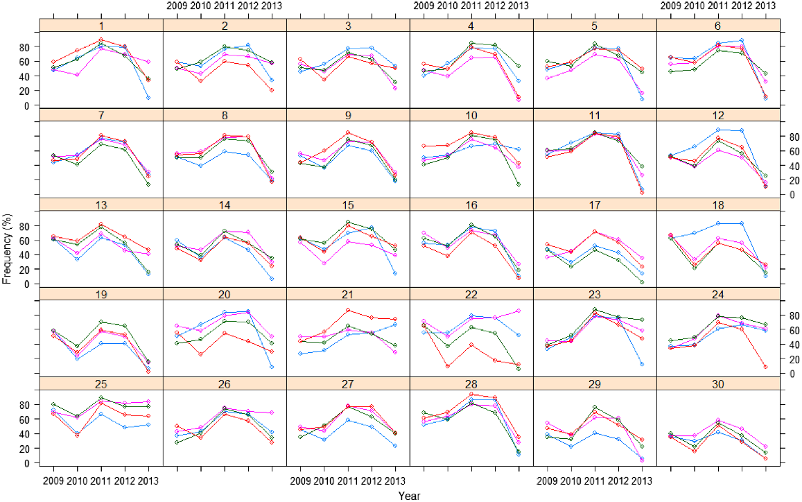
A plot of the raw frequency data over time for each replicate of each variety is given in Fig. 1. The variety profiles are relatively smooth over time and most varieties follow a similar trend. There are differences between individual plot responses within a variety, with some plots having a higher frequency response over the course of the trial and others consistently lower.
Statistical analyses
The phalaris frequency data was analysed using a multi-time analysis, similar to that in De Faveri et al. (2015) but with improved, novel spatio-temporal residual modelling. The variety effects were modelled over time accounting for any spatial and temporal correlation present. The analysis was based on a linear mixed model with estimation using residual maximum likelihood (REML). The analyses were performed in ASReml-R (Butler et al. 2017).
A linear mixed model for the data y (combined across assessment times) may be written as:
where τ is a vector of fixed effects with design matrix X; ug is a vector of random variety (or genetic) effects for t individual assessment-time combinations, with design matrix Zg; uo is a vector of other non-genetic random effects (e.g. replicate effects) with design matrix Zo; and e is the vector of random residual effects.
The random effects from the linear mixed model are assumed to follow a normal distribution with zero mean vector and variance–covariance matrix:
The variance model for the random non-genetic effects is given by a block diagonal matrix Go. The variance matrix Gg for the genetic effects (ug) across times may be represented by where Gh is the genetic variance matrix indexed by the times, and Im is the assumed structure for the varieties. Note that pedigree and/or genomic information could be included here, if available, to relate varieties via relationship matrices; see for example Oakey et al. (2006).
The genetic variance matrix Gh (which consists of genetic variances for each assessment time and genetic co-variances between assessment time combinations) may be modelled using a variety of approaches including unstructured or factor analytic models (Smith et al. 2001, 2015). In Smith et al. (2007), Gh is modelled using an unstructured (US) matrix, but they note that factor analytic (FA) models may also be suitable.
An alternative approach for modelling the genetic effects over time is to use a random regression model. In this approach, the genotype deviations from the underlying mean trend over time are modelled. Often whilst the underlying mean trend may be non-linear, the genotype deviations may be linear over time (Evans and Roberts 1979), but they may vary over varieties. Because we are interested in selection of varieties, the intercept and slope of these deviation responses may be taken as random rather than fixed, similar to the basic quantitative genetics model in which genotype effects are taken as a random factor. If the genetic effects ug have components ug,ik for genotype i, time k (k = 1,…,t), where the actual time is xk, a linear random regression model is:
where ui0 and ui1 are the random intercept and slopes for genotype i, and ue,ik is a residual deviation from the linear random regression, that is, a lack-of-fit term. The intercepts ui0 provide a prediction of performance at xk = 0, so typically the time variable is centred, so that the origin is at the midpoint, or average of the times. The slopes ui1 provide the rate of change of the effect of the genotype, and hence the speed at which the performance changes over time.
This linear random regression model (2) may be extended to a polynomial random regression model to model non-linear trends, or alternatively, it may be preferable to use natural cubic splines (Verbyla et al. 1999) to provide a more flexible approach (De Faveri et al. 2015, 2023).
A random regression model incorporating cubic smoothing splines, for ug,ik (the random effect for variety i at assessment k (k = 1,…,t)) with xk denoting the time at assessment k, can be written as:
For each variety i, usi (a (t − 2) × 1 vector) is the random spline component of the mixed model formulation of the cubic smoothing spline (Verbyla et al. 1999).
The residual covariance matrix R models the spatial correlation and temporal correlation between repeated measurements. This residual covariance matrix has been modelled in this paper using two approaches, including:
1. A three-way separable spatio-temporal process (De Resende et al. 2006; Smith et al. 2007; De Faveri et al. 2015). Therefore, the structure is assumed to be:
where Rh is a covariance matrix that incorporates temporal correlation (between assessment times) and, possibly, heterogeneous variance across times, and Σc and Σr are the column and row local spatial correlation matrices, here taken as autoregressive models of order 1 (ar1) with spatial correlation parameters ϕr and ϕc in the row and column directions, respectively (Gilmour et al. 1997). In the analyses, the temporal covariance components (Rh) have been modelled using unstructured, heterogeneous autoregressive and ante-dependence models (Gabriel 1962). In these analyses, the separable residual models assume the same spatial correlation parameters (ϕr and ϕc) for each assessment time.
2. A two-directional invariant multivariate autoregressive of order 1 (2DIMVAR1) model (De Faveri et al. 2017), where eij, the multivariate error variable for row i and column j for t times is given by:
where ϵ has zero-mean vector and ϵij are mutually independent vector variates, var(eij) = Σ, for all i and j, and Ωr and Ωc are t × t matrices of spatial dependence parameters in the row and column direction, respectively.
It can be shown that under this model, R can be written as the sum of t terms, each the Kronecker product of two autoregressive models and a reduced rank factor analytic model:
This model allows for different spatial correlation parameters for each assessment time.
Full details of the 2DIMVAR1 model can be found in De Faveri et al. (2017); in summary, the model fits a multivariate analogue of the first-order autoregressive spatial model in row and column directions across times (t), with the spatial correlation parameters (ϕr and ϕc) replaced by t × t spatial matrices Ωr and Ωc. The diagonal elements of Ωr give the spatial dependency parameters between neighbouring plots in the row direction at each time, while the off diagonals give the spatial dependency between neighbouring plots at different times, hence allowing for differing spatial correlation across the times (similarly for Ωc). These spatial dependency matrices are not correlation matrices and do not need to be symmetric. Together with a fully unstructured covariance matrix Σ (which models the temporal variance and covariances between times on each plot), the residual spatio-temporal process is modelled. Symmetry constraints on ΩrΣ and ΩcΣ (the spatio-temporal covariance matrices between neighbouring plots in the row and column directions, respectively) make the model directionally invariant in the row and column directions, so the full variance–covariance matrix is the same whether observations are ordered from left to right or from right to left along the rows or columns.
To test the significance of random effects in the linear mixed model, the residual maximum likelihood ratio test (REMLRT) can be used. The REMLRT may be used to compare the fit of two models only if they are nested and contain the same fixed effects. The standard REMLRT statistic is asymptotically distributed as a chi-squared statistic with p1 − p0 degrees of freedom. However, if the test involves a null hypothesis where the parameter is on the boundary of the parameter space, the REMLRT needs to be adjusted (see Stram and Lee 1994).
To compare the goodness of fit of two models (with the same fixed effects) that may be non-nested, the Akaike information criterion (AIC) may be used. The AIC value for a model is calculated as −2(l − p), where l is the residual log-likelihood for the model and p is the number of variance parameters in the model. To compare models with different fixed effects, an AIC based on the full likelihood may be used (Verbyla 2019). Models with smaller AIC values provide a better fit to the data than those with higher AIC values.
Results
The analysis of frequency was based on the linear mixed model given in Eqn 1. A series of genetic and residual models was fitted to the data and results are presented in Table 2. In each analysis, the random experimental design terms for Rep, Row and Column for each year were included in the model.
| Model | Genetic model (G) | Residual model (R) | Other random terms | LL | AIC | |
|---|---|---|---|---|---|---|
| M1 | Diag(Year):Line | id(Col) × id(Row) | Year | At(Year): (Rep + Row + Col) | −1741.564 | 3545.429 | |
| M2 | Diag(Year):Line | ar1(Col):ar1(Row)| Year | At(Year): (Rep + Row + Col) | −1700.932 | 3479.507 | |
| M3 | Diag(Year):Line | ar1(Col):ar1(Row)| Year | At(Year): (Rep + Row + Col) + Plot | −1603.266 | 3274.839 | |
| M4 | Diag(Year):Line | diag(Year):ar1(Col):ar1(Row) | At(Year): (Rep + Row + Col) + Plot | −1612.799 | 3283.941 | |
| M5 | US(Year):Line | ar1h(Year):ar1(Col):ar1(Row) | At(Year): (Rep + Row + Col) + Plot | −1585.288 | 3245.676 | |
| M6 | US(Year):Line | ante(Year,1):ar1(Col):ar1(Row) | At(Year): (Rep + Row + Col) + Plot | −1545.252 | 3173.160 | |
| M7 | US(Year):Line | corgh(Year):ar1(Col):ar1(Row) | At(Year): (Rep + Row + Col) + Plot | −1542.028 | 3175.831 | |
| M8 | US(Year):Line | 2DIMVAR1 | At(Year): (Rep + Row + Col) | −1526.688 | 3115.341 | |
| M9 | RR | ar1h(Year):ar1(Col):ar1(Row) | At(Year): (Rep + Row + Col) + Plot | −1631.308 | 3314.643 | |
| M10 | RR | ante(Year,1):ar1(Col):ar1(Row) | At(Year): (Rep + Row + Col) + Plot | −1580.344 | 3220.703 | |
| M11 | RR | corgh(Year):ar1(Col):ar1(Row) | At(Year): (Rep + Row + Col) + Plot | −1576.359 | 3220.761 | |
| M12 | RR | 2DIMVAR1 | At(Year): (Rep + Row + Col) | −1547.583 | 3173.185 |
Models M1–M4 fit separate genetic effects for each assessment time (Year), whereas models M5–M8 fit a fully unstructured covariance model for the genetic effects across times and models M9–M12 fit a random regression (RR) model for genetic effects over time: Line + lin(time):Line + spl(time):Line + lack of fit term dev(time):Line. In models M1–M8 a separate fixed effect mean for each assessment time (Year) has been fitted, whereas in models M9–M12 the overall mean has been modelled over time using the spline model: 1 + lin(time) + spl(time) + lack of fit term dev(time). Model terms are detailed in the Supplementary material.
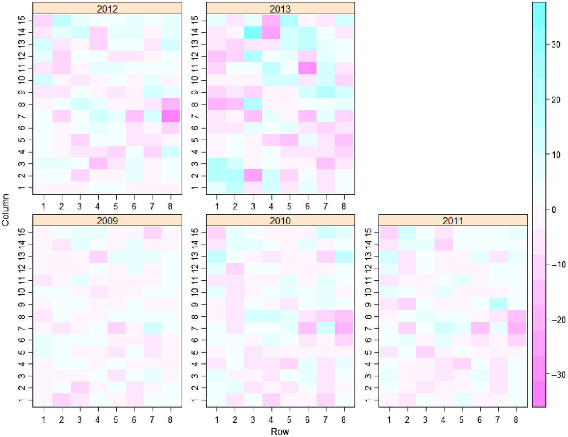
Initially a separate analysis at each time was conducted with a non-spatial model (M1). The residuals from this model are presented in Fig. 2, where it can be seen that the spatial pattern of residuals differs between assessment times. In addition to accounting for the trial design, the next model (M2) followed the spatial analysis approach of Gilmour et al. (1997) and Stefanova et al. (2009), including terms for extraneous and global trend and modelling local spatial correlation using a separable autoregressive process of order 1 in the row and column directions.
Comparing results between model M1 and model M2 clearly shows that accounting for the spatial correlation between plots results in a significant improvement (P < 0.001; REMLRT = 81.264 on 10 d.f.). This initial spatial analysis provides insight into the spatial correlation at each Year. The spatial correlation parameters and residual variances estimated for each assessment time from the initial single time analyses are given in Table 3. From these results, the residual variance can be seen to increase over time. The spatial correlation parameters can also be seen to vary across years with ϕc ranging from 0.261 to 0.622 and ϕr ranging from −0.118 to 0.385. This difference in spatial parameters across times indicates that there may be a need to allow for flexible modelling of the spatial parameters over time.
| Year | Residual variance | Column spatial parameter ϕc | Row spatial parameter ϕr | |
|---|---|---|---|---|
| 2009 | 37.364 | 0.261 | 0.385 | |
| 2010 | 84.575 | 0.528 | −0.048 | |
| 2011 | 67.568 | 0.562 | −0.118 | |
| 2012 | 106.915 | 0.582 | 0.046 | |
| 2013 | 261.859 | 0.622 | 0.049 |
The next model (M3) fitted an overall Plot term, which was significant (REMLRT). The following model (M4) fitted a separable spatial and temporal model allowing for different residual variances for each time but did not model the correlation between times. This separable residual model assumed common row and column spatial parameters across all times, with the common spatial correlation parameters estimated as (ϕc = 0.400, and ϕr = 0.067). This model was not a significant improvement over M3, which allowed for separate spatial parameters across times, indicating that the separable residual models may not be ideal in this situation.
Subsequent models fitted more suitable genetic covariance models to the genetic effects over time, correlating the genetic effects over time.
Models 5, 6 and 7 fitted an unstructured covariance structure to the genetic effects over time, together with different residual models. In this trial the number of measurement times was low (five times), so it was possible to fit the unstructured genetic model. In situations of more measurement times, the number of parameters requiring estimation in the unstructured model is likely to be prohibitive and more parsimonious models are desired (e.g. factor analytic (FA) models). In these three unstructured genetic models, the residual effects have been modelled using a three-way separable spatial and temporal residual model (similar to M4), but in these models the temporal covariance structure is modelled firstly using a heterogeneous autoregressive model of order1 (ar1h) (M5), then an ante-dependence model of order 1 (M6), and then a fully parameterised unstructured model (M7). Based on AIC values, the ante-dependence model was best out of these separable residual models.
The next model (M8) incorporated the multivariate extension of the spatial model, the directionally invariant 2DIMVAR1 residual model, once again with an unstructured genetic model. This residual model allows for differing spatial parameters for each time, hence providing a more flexible spatial and temporal structure. The 2DIMVAR1 model was a significant improvement on the other residual models (REMLRT P < 0.001 in each case).
The final three models fitted a more parsimonious structure to the genetic effects over time using a random regression approach. This approach models the smooth trend across time, allowing for predictions at times other than the measurement times. The models include an underlying overall mean level cubic smoothing spline across times, and random variety deviations are modelled (also using cubic smoothing splines) about this overall mean response, as in Eqn 3. The random variety effects (intercepts and slopes) have been correlated to make the model invariant to translation. It would also be desirable to correlate the random spline components with the random intercepts and slopes to make the model invariant to a change in basis (Fitzmaurice et al. 2009), but this correlation was unable to be fitted. Once again in this set of models, the model with the non-separable 2DIMVAR1 residual model was a significant improvement on the models with separable autoregressive (M9), ante-dependence (M10) and unstructured (M11) by , residual models (REMLRT P < 0.001 in each case).
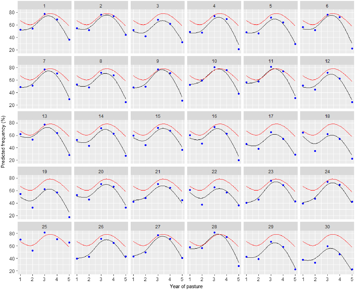
Variety predictions over time have been made from the best random regression model (M12) and smooth responses for each variety plotted in Fig. 3. Predictions from the best unstructured genetic model (M8) have also been included in this plot. Both of these models included the 2DIMVAR1 residual model. In this figure, the control variety (25) response is also plotted in each panel for comparison. The varieties all follow a similar trend, so to compare varieties, it is more informative to investigate the variety deviations from the underlying mean trend. These variety deviations (from M12) are presented in Figs 4 and 5.
Plot of predictions for each variety (black line) and control (25) (red line) from the random regression model with 2DIMVAR1 residual model (M12) together with predictions at each assessment time (blue points) from the unstructured genetic model with 2DIMVAR1 residual model (M8).
Plot of variety deviations from overall mean response over time from model M12 together with 95% prediction intervals.
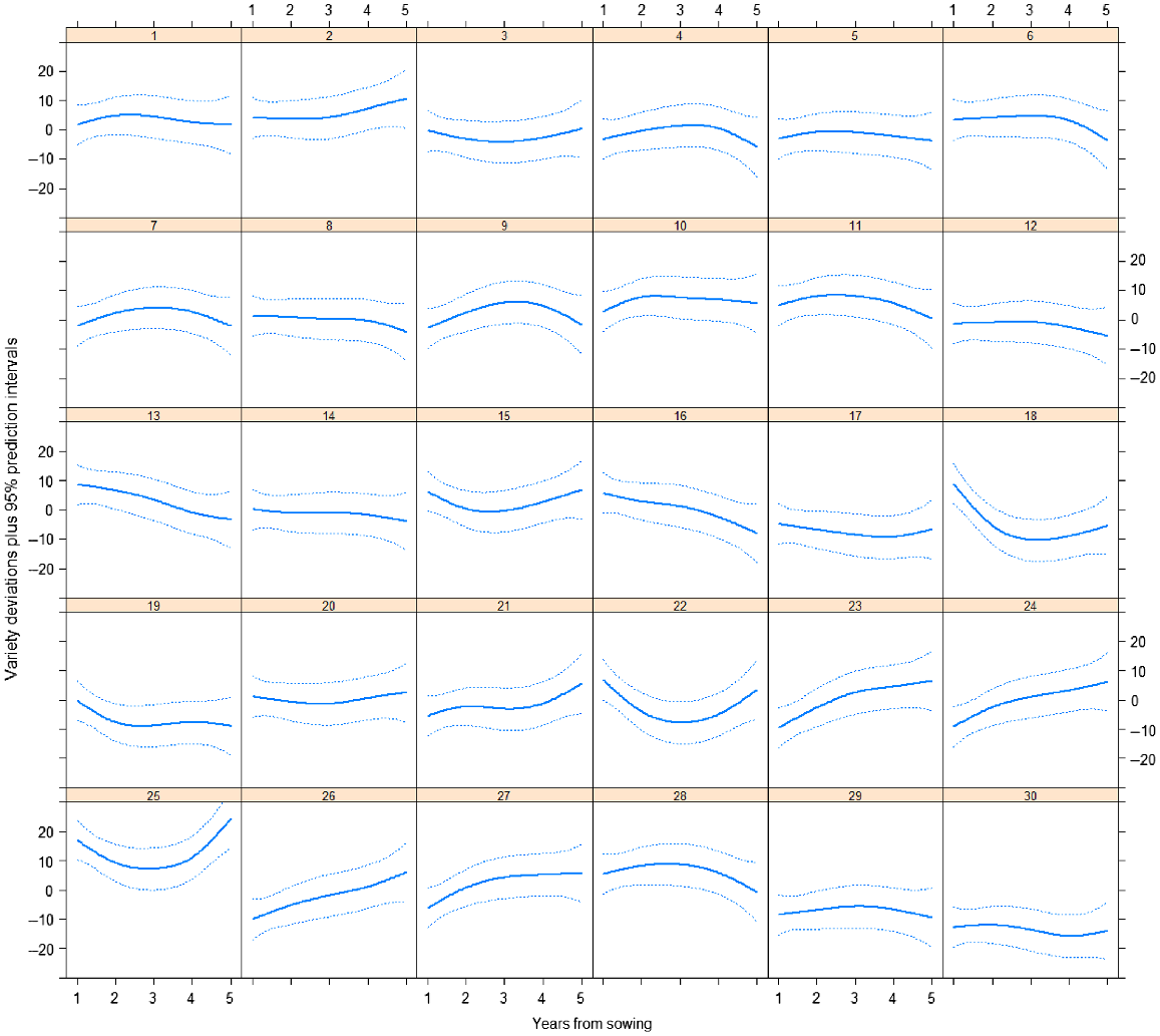
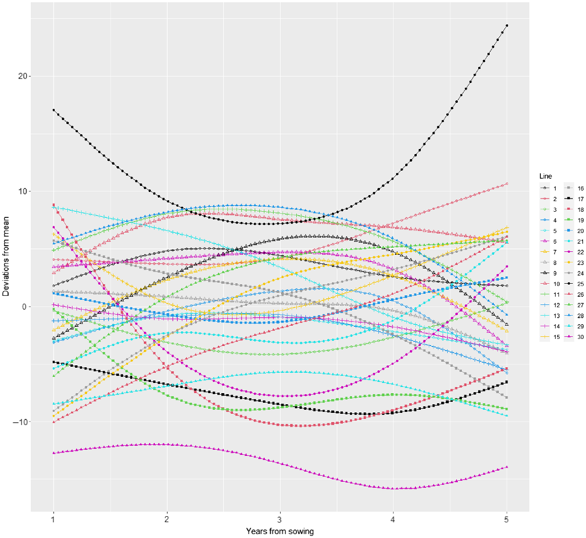
There is considerable variety × year interaction as seen in the crossovers between deviation curves in Fig. 5. The persistent control (25) is high in persistence throughout the trial and especially at the start and end, when it is higher than all other varieties. Some varieties are consistently low (e.g. 30) whereas some start low and continually increase relative to the mean (e.g. 26 and 27). Some varieties do better in the middle years (e.g. 28, 11, 10) and some do better at the end (e.g. 2). Some start high and then decrease (e.g. 18, 16, 13).
As an overall measure of frequency to provide a single comparison measure to rank varieties over time, the area under each predicted variety response curve (from M12) has been calculated. A plot of this total area under curve (AUC) versus final frequency is presented in Fig. 6, giving an insight into those varieties with overall high frequency and high final counts at the end of the trial.
Plot showing the area under the curve versus predicted final frequency for each variety predicted from model M12.
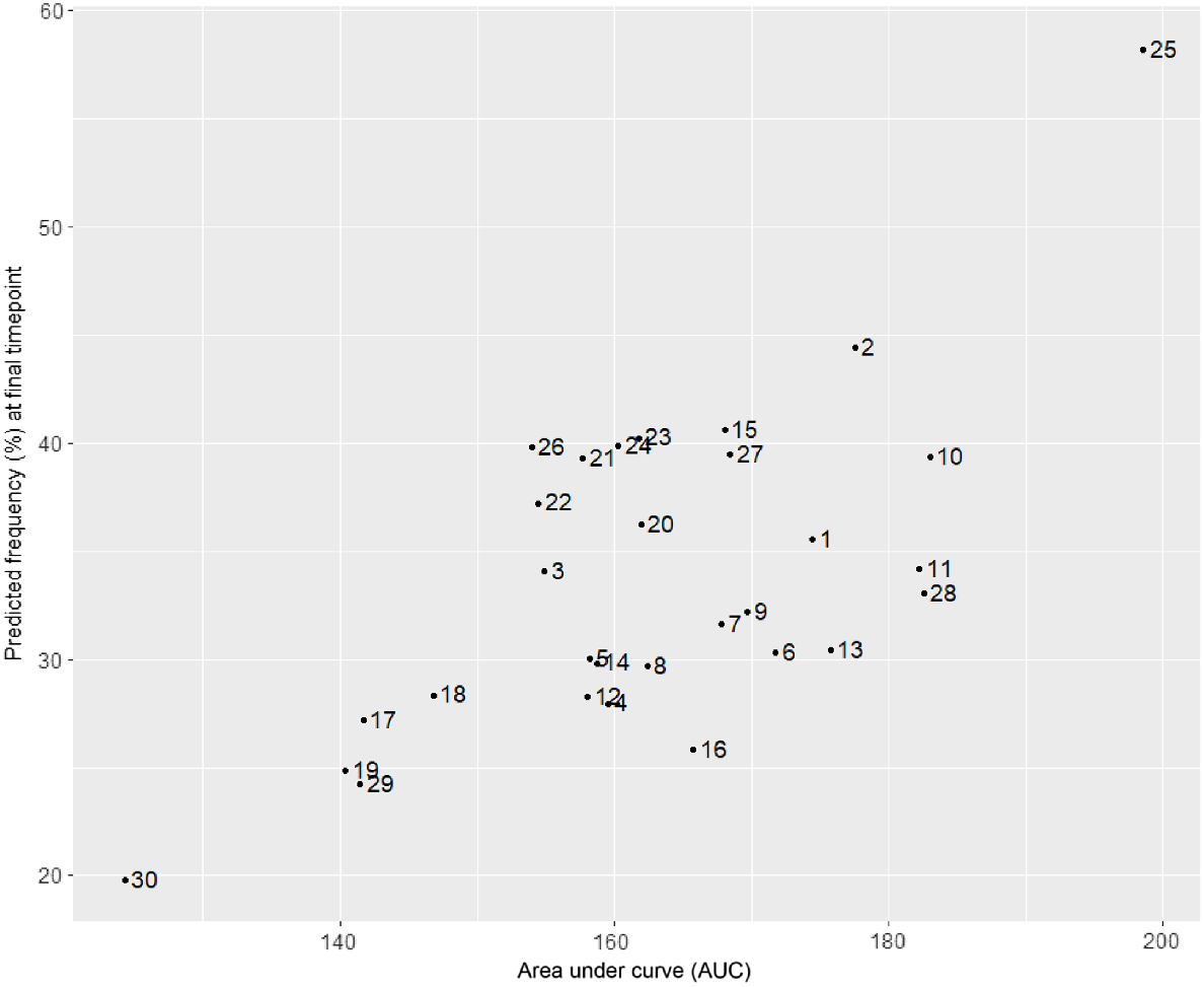
The control variety (25) can be seen to have the greatest AUC and final frequency, while variety 30 has very low AUC and final frequency. Varieties 2 and 10 have high AUC and also high final frequency, whereas varieties 11 and 28 have high AUC but slightly lower final frequency.
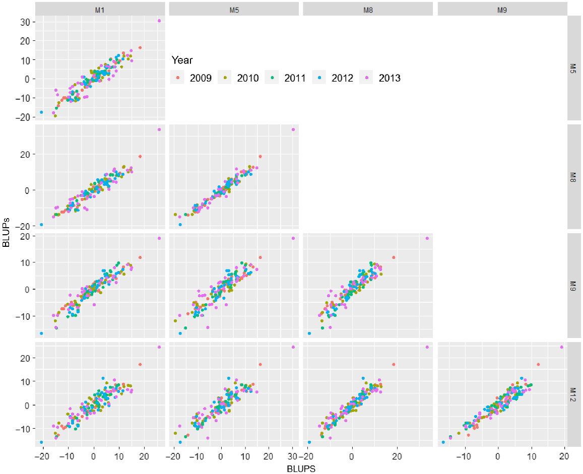
To provide insight into how the choice of residual model may affect the variety predictions, the best linear unbiased predictions (BLUPs) from models M1 (separate non-spatial analysis at each time), M5 and M8 (US genetic model with 3-way separable and 2DIMVAR1 residual model, respectively), and M9 and M12 (CSS random regression genetic model with 3-way separable and 2DIMVAR1 residual model, respectively) have been plotted together in Fig. 7. There are clear differences in the genetic effects depending on the residual model fitted.
Plot of variety BLUPs for each year (represented by colour) from models M1 (separate analysis at each time), M5 and M8 (US genetic model with 3-way separable and 2DIMVAR1 residual model, respectively), and M9 and M12 (CSS random regression genetic model with 3-way separable and 2DIMVAR1 residual model, respectively).
Predicted residual spatial dependency matrices and spatio-temporal correlations from the final model (M12) are presented in the Supplementary material.
Discussion
The analyses presented in this paper of frequency from a perennial pasture variety trial have shown the 2DIMVAR1 residual model to be superior to all of the separable spatial and temporal models fitted under a selection of different genetic models. The models have been compared using AIC values based on the full likelihood (Verbyla 2019). The impact of the different residual models on prediction of genetic effects has been shown in plots of the BLUPs from competing models.
The 2DMVAR1 models were fitted in the software package ASReml-R, taking only seconds per iteration. As the number of measurement times increases, the number of parameters required for estimation in the 2DIMVAR1 model also increases, thereby increasing the computation time and decreasing the feasibility of fitting the 2DMVAR1 model in this form for large numbers of times. It is estimated that any more than 10–12 measurement times may cause computational difficulties using this formulation. Alternative, more parsimonious forms of the 2DIMVAR1 model may be possible (De Faveri 2013) but at this time are unable to be implemented in ASReml-R. This is an area of future research.
The flexibility provided by the 2DIMVAR1 residual model makes sense biologically by allowing for differing spatial correlation at each measurement time. It would be expected that local spatial correlation may be impacted by factors such as soil moisture levels that may vary over time and stage of growth of the plants. The current approach of modelling the spatial and temporal correlation using separable residual models that assume common spatial parameters over time is likely to be restrictive. In many cases, the extra flexibility provided by the 2DIMVAR1 model will provide a statistically better model.
The 2DIMVAR1 residual models in conjunction with random regression genetic models using cubic smoothing splines are easily implemented in the linear mixed model framework, providing an efficient approach for modelling variety profiles over time. The models allow overall rankings to be made across times (for overall performance) and also provide an approach to investigate genotype × time interactions. The models have been implemented here assuming independence between varieties but can easily be extended to include pedigree or genomic relationship information between varieties. The approach can also be extended to the multi-environment situation so that genotype × environment × time interactions may be investigated.
Although the random regression genetic models did not fit as well (based on AIC) as the fully unstructured genetic models in this example (this may be a result of very few measurement times), they enabled in-depth investigation into variety × time interactions and predictions between assessment times. With higher numbers of measurement times, the unstructured model will require too many parameters to be estimated, and the benefit of the more parsimonious genetic models such as the random regression approach is likely to be more evident.
Conclusion
Spatial and temporal correlation affects the prediction of genetic effects over time from perennial pasture field trials, so it is important to model this correlation appropriately. The 2DIMVAR1 residual model provides a flexible covariance structure for modelling this spatial and temporal correlation, allowing for differing spatial correlation across measurement times. This model has been shown to be a significant improvement on more traditional separable spatio-temporal models and, together with parsimonious random regression genetic models, enables investigation into variety × time interactions in perennial crop evaluation.
References
Bally ISE, De Faveri J (2021) Genetic analysis of multiple fruit quality traits in mango across sites and years. Euphytica 217, 44.
| Crossref | Google Scholar |
Bjornsson H (1978) Analysis of a series of long-term grassland experiments with autocorrelated errors. Biometrics 34, 645-651.
| Crossref | Google Scholar |
Campbell M, Walia H, Morota G (2018) Utilizing random regression models for genomic prediction of a longitudinal trait derived from high-throughput phenotyping. Plant Direct 2, 1-11.
| Crossref | Google Scholar |
Costa e Silva J, Dutkowski G, Gilmour AR (2001) Analysis of early tree height in forest genetic trials is enhanced by including a spatially correlated residual. Canadian Journal of Forest Research 31, 1887-1893.
| Crossref | Google Scholar |
Culvenor RA, Norton MR, De Faveri J (2017) Persistence and productivity of phalaris (Phalaris aquatica) germplasm in dry marginal rainfall environments of south-eastern Australia. Crop & Pasture Science 68, 781-797.
| Crossref | Google Scholar |
De Faveri J (2013) Spatial and temporal modelling for perennial crop variety selection trials. PhD Thesis, The University of Adelaide, Adelaide, SA, Australia. Available at http://digital.library.adelaide.edu.au/dspace/handle/2440/83114
De Faveri J, Verbyla AP, Pitchford WS, Venkatanagappa S, Cullis BR (2015) Statistical methods for analysis of multi-harvest data from perennial pasture variety selection trials. Crop & Pasture Science 66, 947-962.
| Crossref | Google Scholar |
De Faveri J, Verbyla AP, Cullis BR, Pitchford WS, Thompson R (2017) Residual variance–covariance modelling in analysis of multivariate data from variety selection trials. Journal of Agricultural, Biological and Environmental Statistics 22, 1-22.
| Crossref | Google Scholar |
De Faveri J, Verbyla AP, Rebetzke G (2023) Random regression models for multi-environment, multi-time data from crop breeding selection trials. Crop & Pasture Science 74, 271-283.
| Crossref | Google Scholar |
De Resende MDV, Thompson R, Welham SJ (2006) Multivariate spatial statistical analysis of longitudinal data in perennial crops. Revista de Matemática e Estatística, São Paulo 24(1), 147-169 Available at https://repository.rothamsted.ac.uk/item/8q3zq.
| Google Scholar |
DeGroot BJ, Keown JF, Kachman SD, Van Vleck D (2003) Cubic splines for estimating lactation curves and genetic parameters of first lactation Holstein cows treated with bovine somatotropin. In ‘Conference on applied statistics in agriculture’. pp. 150–163. (New Prairie Press: Kansas, USA). doi:10.4148/2475-7772.1181
Diggle PJ (1988) An approach to the analysis of repeated measurements. Biometrics 44, 959-971.
| Crossref | Google Scholar |
Dutkowski GW, Silva JCe, Gilmour AR, Lopez GA (2002) Spatial analysis methods for forest genetic trials. Canadian Journal of Forest Research 32, 2201-2214.
| Crossref | Google Scholar |
Evans JC, Roberts EA (1979) Analysis of sequential observations with applications to experiments on grazing animals and perennial plants. Biometrics 35, 687-693.
| Crossref | Google Scholar |
Gabriel KR (1962) Ante-dependence analysis of an ordered set of variables. The Annals of Mathematical Statistics 33, 201-212.
| Crossref | Google Scholar |
Gilmour AR, Cullis BR, Verbyla AP (1997) Accounting for natural and extraneous variation in the analysis of field experiments. Journal of Agricultural, Biological, and Environmental Statistics 2, 269-293.
| Crossref | Google Scholar |
Haskard KA, Cullis BR, Verbyla AP (2007) Anisotropic Matérn correlation and spatial prediction using REML. Journal of Agricultural, Biological, and Environmental Statistics 12(2), 147-160.
| Crossref | Google Scholar |
Huisman AE, Veerkamp RF, van Arendonk JAM (2002) Genetic parameters for various random regression models to describe the weight data of pigs. Journal of Animal Science 80, 575-582.
| Crossref | Google Scholar |
Laird NM, Ware JH (1982) Random-effects models for longitudinal data. Biometrics 38, 963-974.
| Crossref | Google Scholar |
Lodge GM, Gleeson AC (1984) A comparison of methods of estimating lucerne population for monitoring persistence. Australian Journal of Experimental Agriculture and Animal Husbandry 24, 174-177.
| Crossref | Google Scholar |
Meyer K (2005) Random regression analyses using B-splines to model growth of Australian Angus cattle. Genetics Selection Evolution 37, 473.
| Crossref | Google Scholar |
Oakey H, Verbyla A, Pitchford W, Cullis B, Kuchel H (2006) Joint modeling of additive and non-additive genetic line effects in single field trials. Theoretical and Applied Genetics 113, 809-819.
| Crossref | Google Scholar |
O’Connor KM, Hayes BJ, Hardner CM, Alam M, Henry RJ, Topp BL (2021) Genomic selection and genetic gain for nut yield in an Australian macadamia breeding population. BMC Genomics 22, 370.
| Crossref | Google Scholar |
R Core Team (2021) ‘R: a language and environment for statistical computing.’ (R Foundation for Statistical Computing: Vienna, Austria) Available at https://www.R-project.org/
Smith KF, Simpson RJ, Oram RN, Lowe KF, Kelly KB, Evans PM, Humphreys MO (1998) Seasonal variation in the herbage yield and nutritive value of perennial ryegrass (Lolium perenne L.) cultivars with high or normal herbage water-soluble carbohydrate concentrations grown in three contrasting Australian dairy environments. Australian Journal of Experimental Agriculture 38, 821-830.
| Crossref | Google Scholar |
Smith A, Cullis B, Thompson R (2001) Analyzing variety by environment data using multiplicative mixed models and adjustments for spatial field trend. Biometrics 57, 1138-1147.
| Crossref | Google Scholar |
Smith AB, Cullis BR, Thompson R (2005) The analysis of crop cultivar breeding and evaluation trials: an overview of current mixed model approaches. The Journal of Agricultural Science 143, 449-462.
| Crossref | Google Scholar |
Smith AB, Stringer JK, Wei X, Cullis BR (2007) Varietal selection for perennial crops where data relate to multiple harvests from a series of field trials. Euphytica 157, 253-266.
| Crossref | Google Scholar |
Smith AB, Ganesalingam A, Kuchel H, Cullis BR (2015) Factor analytic mixed models for the provision of grower information from national crop variety testing programs. Theoretical and Applied Genetics 128, 55-72.
| Crossref | Google Scholar |
Stefanova KT, Smith AB, Cullis BR (2009) Enhanced diagnostics for the spatial analysis of field trials. Journal of Agricultural, Biological, and Environmental Statistics 14, 392-410.
| Crossref | Google Scholar |
Stram DO, Lee JW (1994) Variance components testing in the longitudinal mixed effects model. Biometrics 50, 1171-1177.
| Crossref | Google Scholar |
Verbyla AP (2019) A note on model selection using information criteria for general linear models estimated using REML. Australian & New Zealand Journal of Statistics 61, 39-50.
| Crossref | Google Scholar |
Verbyla KL, Verbyla AP (2009) Estimated breeding values and association mapping for persistency and total milk yield using natural cubic smoothing splines. Genetics Selection Evolution 41, 48.
| Crossref | Google Scholar |
Verbyla AP, Cullis BR, Kenward MG, Welham SJ (1999) The analysis of designed experiments and longitudinal data by using smoothing splines. Journal of the Royal Statistical Society Series C: Applied Statistics 48, 269-311.
| Crossref | Google Scholar |
Verbyla AP, De Faveri J, Deery DM, Rebetzke GJ (2021) Modelling temporal genetic and spatio-temporal residual effects for high-throughput phenotyping data. Australian & New Zealand Journal of Statistics 63, 284-308.
| Crossref | Google Scholar |
Welham SJ, Gogel BJ, Smith AB, Thompson R, Cullis BR (2010) A comparison of analysis methods for late-stage variety evaluation trials. Australian & New Zealand Journal of Statistics 52(2), 125-149.
| Crossref | Google Scholar |
White IMS, Thompson R, Brotherstone S (1999) Genetic and environmental smoothing of lactation curves with cubic splines. Journal of Dairy Science 82, 632-638.
| Crossref | Google Scholar |