

Evaluating the Agricultural Production Systems sIMulator (APSIM) wheat module for California
Nicholas Alexander George A B * , Helio de Jesus Pedro Cuamba B C , Mark E. Lundy A D and Sarita Jane Bennett B
A
B
C
D
Abstract
Computer-based crop simulation models are important tools for agricultural research and management. APSIM (Agricultural Production Systems sIMulator) is commonly used around the world but has not been widely validated in North America.
The objective of this work was to evaluate the reliability of APSIM for simulating wheat production in California, with the aim of providing guidance for future field research aimed at model calibration and validation.
Environmental and management data from state-wide wheat variety trials of common wheat (Triticum aestivum L.) were used to parameterise the APSIM-Wheat module (ver. 7.10 r4220). Simulated yield and protein data were compared with observed field trial results to test the reliability of APSIM simulations.
The most reliable simulation of grain yield had a root-mean-square error of 1040 kg/ha and normalised root-mean-square error of 16% relative to actual field data. Preliminary calibration of the model for Californian wheat varieties did not improve simulation accuracy or precision.
The accuracy or precision of the simulations was comparable to that of other tests of the APSIM-Wheat module in environments where it has not been previously calibrated but was considered too low to be reliable. The lack of reliability was due to the poor representation of local Californian wheat genotypes by existing APSIM cultivars, as well as possible lack of precision and accuracy of field data.
APSIM could be a valuable tool for wheat research and management in California; however, further research is needed to generate suitable field data for model calibration and validation.
Keywords: abiotic stress, agronomy, breeding, cereals, cropping systems, farming systems, mediterranean environments.
Introduction
Computer-based crop simulation models are well-established tools for agricultural research and management and are becoming increasingly important for improving agricultural productivity and addressing challenges such as climate change (Reardon-Smith et al. 2015; Robertson et al. 2015; Ahmed et al. 2016; Muller and Martre 2019; Keating 2020). They permit the exploration of complex bio-physical processes, which can at times be difficult, time-consuming or expensive to study in the field (Pasquel et al. 2022). One of the more widely used of these models is the Agricultural Production Systems sIMulator (APSIM), developed by the Agricultural Production Systems Research Unit, Toowoomba, Queensland, Australia. APSIM has been successfully applied to a range of common crop species and complex agricultural systems around the world (Keating et al. 2003; Holzworth et al. 2014, 2018).
California, USA, is one of the world’s most commercially valuable agricultural regions (USDA NASS 2020), being a leading generator of farm cash receipts for several decades for products including vegetables, nuts, fruits, and small grains, totalling US$50 billion in 2021 (CDFA 2022). The dominant grain crop in California is wheat (Jackson et al. 2006; CDFA 2022); it plays an important role in the agricultural systems of the region as one of the few crops adapted to cool-season and predominantly rainfed production (Jackson et al. 2006). The region has recently experienced drought events that are attributed in part to climate change (Williams et al. 2022). Climate change is likely to lead to increasing temperatures and decreasing rainfall in the region, negatively impacting irrigated perennial and summer crops (Pathak et al. 2018). In addition, the 2014 Sustainable Groundwater Management Act has also directly reduced irrigation availability (Harter 2020). The winter rotational niche, when crops can be grown using rainfall and during times of lower evapotranspiration, could therefore become increasingly important for the viability of agribusinesses in California.
APSIM has potential for multiple practical applications for the Californian wheat industry, including identification of optimal strategies for irrigation and nitrogen fertility management (Asseng et al. 2001; Peake et al. 2014; Lawes et al. 2019; Zhao et al. 2020); optimisation of crop rotations (Yunusa et al. 2004; Kotir et al. 2020); informing plant breeding objectives (Chenu et al. 2018; Hammer et al. 2020; Ramirez-Villegas et al. 2020); in-season decision support for growers (Hochman et al. 2009a); and better understanding the impacts of climate change and identifying mitigation strategies (Zheng et al. 2012; Ahmed et al. 2016; Ramirez-Villegas et al. 2020; Ye et al. 2020). A recent assessment of the general performance of the APSIM-Wheat model found that it successfully predicted crop responses to a diverse range of environmental conditions and management practices (Brown et al. 2018). There has been recent testing and validation of APSIM for simulation of the growth and water use of crops including maize, soybean and canola in North America (Archontoulis et al. 2014a, 2014b; George and Kaffka 2017; George et al. 2018; Balboa et al. 2019). APSIM has been used to simulate wheat production for both research and commercial purposes in regions of Australia that are climatically comparable to California (Asseng et al. 1998; Farré et al. 2002; Hochman et al. 2009b). However, published work testing the accuracy or precision of the model for simulating wheat production in the western United States is scarce.
The application of a crop model to new genotypes and environments requires formal model calibration and validation. In the case of the APSIM-Wheat module, this necessitates relatively ‘high-resolution’ field data for parameters including the phenological response of local genotypes to thermal time, sensitivity to vernalisation and phenology, canopy development and senescence, yield and biomass accumulation over time, and crop response to water and nitrogen (Zheng et al. 2015; Brown et al. 2018). Such data are generally obtained through dedicated field experiments, and are either not routinely collected for wheat in California (Dubcovsky 2020), or are not available across a sufficient number of environments to allow for model calibration and validation. A lack of suitable field data often acts as a barrier to the development and use of crop models (Zhao et al. 2019).
The Small Grains Program of the University of California (UC), Davis, conducts annual state-wide multi-environment field trials and agronomic studies of wheat (George et al. 2017; Nelsen et al. 2018, 2019). This work generates information regarding the performance of local wheat genotypes, along with management and environmental information, across multiple, diverse sites and years throughout California. These data are not collected for crop model testing, and therefore do not fully comprise the type of information needed for calibrating and validating APSIM. However, this study utilises the extensive, multi-environment dataset opportunistically to evaluate the performance of the APSIM-Wheat model in California. Our objective was to test the accuracy and precision of the current APSIM release to inform future field research efforts aimed at the validation and calibration of the model for California.
Materials and methods
Field data
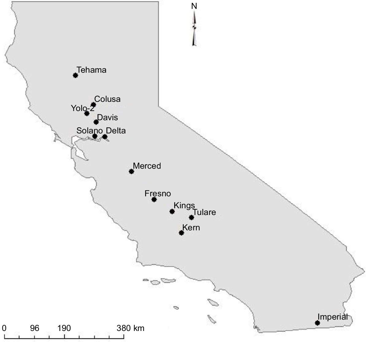
Both public and internal data including grain yield, grain protein and phenology for common wheat (Triticum aestivum L.) were obtained from the state-wide genotype trial results of the UC Small Grains Program, USA (George et al. 2017; Nelsen et al. 2018, 2019). These comprised 12 field locations in the main cereal production regions of California, conducted over three winter seasons from 2016–17 to 2018–19 (Fig. 1, Table 1). In total, 34 environments (location-by-management-by-year combinations) were sampled. The field locations fall between latitudes 33°N and 42°N, a north–south distance of ~800 km. Two locations in the dataset were identified where field yields were considered unlikely in view of the reported environmental and management conditions for the locations as described below. Estimates of the water-limited yield potential, using Sadras (2020), suggested the reported yield at Tulare in 2017 was too high given the reported growing-season rainfall and starting soil water. The yields at the low-nitrogen managed-stress Fresno 2018 site were also considered too high considering the reported nitrogen fertilisation and residual soil nitrogen. Owing to the uncertainty around the reliability of reported environmental and management variables at these locations, they were removed from the simulation.
Locations used as a source of field data to test the performance of the APSIM-Wheat module in California (George et al. 2017; Nelsen et al. 2018, 2019).
| Site | Season | Lat. (°) | Long. (°) | Sowing date | Soil type | |
|---|---|---|---|---|---|---|
| Colusa | 2016–17 | 39.04 | −121.84 | 10 Nov. 2016 | Loam | |
| Davis | 2016–17 | 38.52 | −121.77 | 15 Nov. 2016 | Loam | |
| Davis (ln) | 2016–17 | 38.52 | −121.77 | 15 Nov. 2016 | Loam | |
| Delta | 2016–17 | 38.15 | −121.53 | 18 Nov. 2016 | Clay loam | |
| Fresno | 2016–17 | 36.34 | −120.12 | 1 Dec. 2016 | Clay loam | |
| Fresno (ln) | 2016–17 | 36.34 | −120.12 | 1 Dec. 2016 | Clay loam | |
| Fresno (lw) | 2016–17 | 36.34 | −120.12 | 1 Dec. 2016 | Clay loam | |
| Imperial | 2016–17 | 32.81 | −115.45 | 9 Dec. 2016 | Silty clay | |
| Kern | 2016–17 | 35.38 | −119.33 | 21 Nov. 2016 | Sandy loam | |
| Solano | 2016–17 | 38.14 | −121.74 | 16 Nov. 2016 | Clay | |
| Tulare | 2016–17 | 35.81 | −119.05 | 29 Nov. 2016 | Clay | |
| Colusa | 2017–18 | 38.93 | −121.84 | 22 Nov. 2017 | Loam | |
| Davis | 2017–18 | 38.54 | −121.78 | 21 Nov. 2017 | Loam | |
| Davis (ln) | 2017–18 | 38.54 | −121.78 | 29 Nov. 2017 | Loam | |
| Davis (lw) | 2017–18 | 38.54 | −121.78 | 21 Nov. 2017 | Loam | |
| Delta | 2017–18 | 38.13 | −121.53 | 18 Nov. 2017 | Clay loam | |
| Fresno | 2017–18 | 36.34 | −120.11 | 29 Nov. 2017 | Clay loam | |
| Fresno (ln) | 2017–18 | 36.34 | −120.11 | 1 Dec. 2017 | Clay loam | |
| Fresno (lw) | 2017–18 | 36.34 | −120.11 | 29 Nov. 2017 | Clay loam | |
| Imperial | 2017–18 | 32.81 | −115.44 | 13 Dec. 2017 | Silty clay | |
| Kern | 2017–18 | 35.37 | −119.33 | 28 Nov. 2017 | Sandy loam | |
| Kings | 2017–18 | 35.99 | −119.59 | 5 Dec. 2017 | Clay | |
| Solano | 2017–18 | 38.15 | −121.81 | 21 Nov. 2017 | Clay | |
| Tehama | 2017–18 | 39.88 | −122.36 | 15 Dec. 2017 | Loam | |
| Tulare | 2017–18 | 35.82 | −119.04 | 28 Nov. 2017 | Clay | |
| Colusa | 2018–19 | 39.03 | −121.84 | 26 Nov. 2018 | Loam | |
| Davis | 2018–19 | 38.53 | −121.77 | 13 Dec. 2018 | Loam | |
| Davis (ln) | 2018–19 | 38.53 | −121.77 | 13 Dec. 2018 | Loam | |
| Delta | 2018–19 | 38.19 | −121.49 | 14 Nov. 2018 | Silt loam | |
| Fresno | 2018–19 | 36.34 | −120.08 | 12 Dec. 2018 | Clay loam | |
| Kern | 2018–19 | 35.52 | −119.49 | 20 Nov. 2018 | Sandy loam | |
| Merced | 2018–19 | 37.14 | −120.75 | 19 Nov. 2018 | Clay loam | |
| Yolo 2 | 2018–19 | 38.8 | −122.05 | 27 Nov. 2018 | Silty clay loam |
ln, low-nitrogen managed-stress trial; lw, low-irrigation managed-stress trial.
Environmental and management details are summarised in Tables 1, 2 and 3. Additional trial methodology and field management details are summarised by Nelsen et al. (2019) and George and Lundy (2019). A range of management practices were used across the field sites, including low-input dryland production, with low growing-season rainfall, to high-input and fully irrigated production. At the Davis and Fresno locations, managed-stress trials were also conducted adjacent to conventionally managed trials with the same wheat genotypes. The managed-stress trials consisted of either restricted irrigation or no nitrogen fertilisation.
| Initial soil N | Sowing N rate | Total N rate | Sowing N type | Second application | Third application | Fourth application | ||||||||
|---|---|---|---|---|---|---|---|---|---|---|---|---|---|---|
| Environment | <50 cm depth (μg/g) | (kg N/ha) | Date | Rate (kg N/ha) | Type | Date | Rate (kg N/ha) | Type | Date | Rate (kg N/ha) | Type | |||
| Colusa 2016–17 | 35 | 140 | 175 | NH4NO3 | 25 Feb. | 35 | NH4NO3 | |||||||
| Colusa 2017–18 | 24 | 70 | 130 | NH4 | 28 Feb. | 60 | Urea | |||||||
| Colusa 2018–19 | 89 | 65 | 120 | NH4 | 31 Jan. | 55 | Urea | |||||||
| Davis 2016–17 | 10 | 55 | 225 | Urea | 4 Feb. | 170 | Urea | |||||||
| Davis 2017–18 | 5 | 55 | 220 | Urea | 20 Feb. | 110 | NH4SO4 | 5 Apr. | 55 | Urea | ||||
| Davis 2018–19 | 26 | 30 | 195 | Urea | 22 Feb. | 110 | Urea | 19 Apr. | 55 | Urea | ||||
| Davis (ln) 2016–17 | 10 | 0 | 0 | |||||||||||
| Davis (ln) 2017–18 | 5 | 0 | ||||||||||||
| Davis (ln) 2018–19 | 26 | 0 | ||||||||||||
| Davis (lw) 2017–18 | 5 | 55 | 220 | Urea | 20 Feb. | 110 | NH4SO4 | 5 Apr. | 55 | Urea | ||||
| Delta 2016–17 | 12.5 | 55 | 55 | NH4NO3 | ||||||||||
| Delta 2017–18 | 21 | 140 | 140 | NH4NO3/urea | ||||||||||
| Delta 2018–19 | 19.5 | 0 | ||||||||||||
| Fresno 2016–17 | 4 | 55 | 225 | Urea | 15 Feb. | 170 | Urea | |||||||
| Fresno 2017–18 | 11 | 75 | 26 Feb. | 50 | Urea | 5 Apr. | 25 | Urea | ||||||
| Fresno 2018–19 | 13 | 165 | 25 Feb. | 110 | Urea | 15 Apr. | 55 | Urea | ||||||
| Fresno (ln) 2016–17 | 0.5 | 0 | ||||||||||||
| Fresno (ln) 2017–18 | 11 | 0 | ||||||||||||
| Fresno (lw) 2016–17 | 0.5 | 55 | 165 | Urea | 15 Feb. | 110 | Urea | |||||||
| Fresno (lw) 2017–18 | 11 | 50 | 20 Mar. | 50 | Urea | |||||||||
| Imperial 2016–17 | 30 | 55 | 280 | Urea | 31 Jan. | 75 | Urea | 1 Mar. | 75 | Urea | 30 Mar. | 75 | Urea | |
| Imperial 2017–18 | 30 | 55 | 275 | Urea | 19 Jan. | 110 | NH4 | 13 Feb. | 55 | NH4 | 7 Mar. | 55 | NH4 | |
| Kern 2016–17 | 12 | 85 | 140 | NH4NO3/urea | 14 Mar. | 55 | NH4NO3/urea | |||||||
| Kern 2017–18 | 5 | 120 | 280 | NH4NO3/urea | 21 Feb. | 160 | Urea | |||||||
| Kern 2018–19 | 31 | 120 | 280 | NH4NO3/urea | 21 Feb. | 160 | Urea | |||||||
| Kings 2017–18 | 15 | 95 | 220 | NH4 | 21 Jan. | 35 | NH4 | 21 Feb. | 55 | NH4NO3/urea | 21 Mar. | 35 | NH4 | |
| Merced 2018–19 | 110 | 10 | 10 | Urea | ||||||||||
| Solano 2016–17 | 1.5 | 55 | 190 | Urea | 26 Jan. | 135 | Urea | |||||||
| Solano 2017–18 | 1.5 | 55 | 55 | NH4 | ||||||||||
| Tehama 2017–18 | 3 | 55 | 165 | Urea | 22 Feb. | 110 | Urea | |||||||
| Tulare 2016–17 | 5 | 10 | 10 | NH4 | ||||||||||
| Tulare 2017–18 | 5 | 0 | ||||||||||||
| Yolo 2 2018–19 | 12 | 30 | 105 | NH4 | 9 Feb. | 65 | NH4NO3 | 25 Apr. | 10 | NH4 | ||||
ln, low-nitrogen managed-stress trial; lw, low-water managed-stress trial.
| Environment | Starting SWC (mm) | CIMIS | GSR | Irrigation | GDD | First irrigation | Second irrigation | Third irrigation | Fourth irrigation | Fifth irrigation | Sixth irrigation | |||||||
|---|---|---|---|---|---|---|---|---|---|---|---|---|---|---|---|---|---|---|
| (mm) | Timing | Amount (mm) | Timing | Amount (mm) | Timing | Amount (mm) | Timing | Amount (mm) | Timing | Amount (mm) | Timing | Amount (mm) | ||||||
| Colusa 2016–17 | 0 | Davis | 726 | Rainfed | 2240 | |||||||||||||
| Colusa 2017–18 | 180 | Davis | 228 | Rainfed | 2310 | |||||||||||||
| Colusa 2018–19 | 0 | Davis | 643 | Rainfed | 2030 | |||||||||||||
| Davis 2016–17 | 50 | Davis | 726 | Rainfed | 2240 | |||||||||||||
| Davis 2017–18 | 0 | Davis | 228 | 405 | 2310 | 14 Dec. | 25.4 | 21 Feb. | 152 | 20 Apr. | 228 | |||||||
| Davis 2018–19 | 15 | Davis | 643 | 64 | 2030 | 22 Apr. | 63.5 | |||||||||||
| Davis (ln) 2016–17 | 15 | Davis | 726 | Rainfed | 2240 | |||||||||||||
| Davis (ln) 2017–18 | 10 | Davis | 228 | 405 | 2310 | 14 Dec. | 25.4 | 21 Feb. | 152 | 20 Apr. | 228 | |||||||
| Davis (ln) 2018–19 | 20 | Davis | 643 | 64 | 2030 | 22 Apr. | 63.5 | |||||||||||
| Davis (lw) 2017–18 | 0 | Davis | 228 | 127 | 2310 | 14 Dec. | 25.4 | 21 Feb. | 102 | |||||||||
| Delta 2016–17 | 700 A | Staten | 805 | Rainfed | 2300 | |||||||||||||
| Delta 2017–18 | 700 A | Staten | 229 | Rainfed | 2370 | |||||||||||||
| Delta 2018–19 | 0 | Staten | 570 | Rainfed | 2310 | |||||||||||||
| Fresno 2016–17 | 260 | FivePoints | 179 | 533 | 2290 | 9 Dec. | 88.9 | 16 Feb. | 88.9 | 14 Mar. | 177.8 | 26 Apr. | 177.8 | |||||
| Fresno 2017–18 | 20 | FivePoints | 100 | 244 | 2380 | 6 Dec. | 12 | 7 Dec. | 38 | 14 Dec. | 17 | 20 Feb. | 93 | 10 Apr. | 84 | |||
| Fresno 2018–19 | 0 | FivePoints | 207 | 371 | 2190 | 13 Dec. | 25.4 | 21 Dec. | 19.05 | 8 Jan. | 19.05 | 28 Feb. | 12.7 | 25 Mar. | 172.72 | 16 Apr. | 121.92 | |
| Fresno (ln) 2016–17 | 270 | FivePoints | 179 | 533 | 2290 | 9 Dec. | 88.9 | 16 Feb. | 88.9 | 14 Mar. | 177.8 | 26 Apr. | 177.8 | |||||
| Fresno (ln) 2017–18 | 0 | FivePoints | 100 | 237 | 2380 | 6 Dec. | 8 | 7 Dec. | 35 | 14 Dec. | 17 | 20 Feb. | 93 | 10 Apr. | 84 | |||
| Fresno (lw) 2016–17 | 210 | FivePoints | 179 | 320 | 2290 | 9 Dec. | 25.4 | 16 Feb. | 147.32 | 13 Apr. | 147.32 | |||||||
| Fresno (lw) 2017–18 | 10 | FivePoints | 100 | 153 | 2380 | 6 Dec. | 8 | 7 Dec. | 35 | 14 Dec. | 17 | 20 Feb. | 93 | |||||
| Imperial 2016–17 | 20 | Meloland | 32 | 715 | 2980 | 15 Dec. | 143 | 31 Jan. | 143 | 1 Mar. | 143 | 30 Mar. | 143 | 4 Apr. | 143 | |||
| Imperial 2017–18 | 165 | Meloland | 0 | 938 | 2960 | 14 Dec. | 178 | 19 Jan. | 76 | 13 Feb. | 178 | 7 Mar. | 100 | 27 Mar. | 178 | 13 Apr. | 228 | |
| Kern 2016–17 | 150 | Shafter | 149 | 334 | 2400 | 1 Dec. | 167 | 14 Mar. | 167 | 21 Apr. | 167 | |||||||
| Kern 2017–18 | 0 | Shafter | 94 | 608 | 2450 | 28 Nov. | 152 | 1 Jan. | 152 | 1 Mar. | 152 | 21 Apr. | 152 | |||||
| Kern 2018–19 | 80 | Shafter | 188 | 457 | 2430 | 1 Oct. | 152.4 | 25 Mar. | 152.4 | 15 Apr. | 152.4 | |||||||
| Kings 2017–18 | 0 | Shafter | 41 | 452 | 2370 | 15 Dec. | 100 | 21 Jan. | 152 | 21 Feb. | 100 | 21 Mar. | 100 | |||||
| Merced 2018–19 | 65 | Denair II | 359 | 178 | 2260 | 15 Dec. | 88.9 | 30 Dec. | 88.9 | |||||||||
CIMIS Station indicates the name of the nearest representative weather station (CIMIS 2020).
ln, low-nitrogen managed-stress trial; lw, low-water managed-stress trial.
Soil types at the field locations were predominantly loams, with relatively undifferentiated profiles to a depth of at least 1 m (California Soil Resources Lab 2020). Physical and chemical information for the soils at the field locations was obtained from soil samples taken during the establishment of field sites and the previous work of George and Kaffka (2017). Additional soil information was obtained from the California Soil Resources Lab (2020). Representative starting soil-water data were obtained from soil sampling and reported field measurements (George et al. 2017; Nelsen et al. 2018, 2019). The plant-available soil-water content was estimated by using this information and the crop and soil lower limits. In most locations, starting soil-water content was small relative to rainfall and irrigation.
Weather data were obtained from the California Irrigation Management Information System (CIMIS) weather station network, using the nearest representative station to each location (CIMIS 2020). The locations represent a range of climate types (Mediterranean to desert) (Peel et al. 2007). Growing-season rainfall was estimated from sowing to 1 July of the following year. Growing-season rainfall varied from 0 to 800 mm. Growing degree-days were estimated with daily average temperature, using base 0°C.
Twenty commonly grown wheat genotypes were tested across all three growing seasons (Table 4); however, not all genotypes survived to harvest in all environments. The dataset comprised a range of maturity types and yield potentials, with field yields ranging from 22 to 11 700 kg/ha.
| Cultivar | UC code | |
|---|---|---|
| Yecora Rojo | 112 | |
| SY Cal Rojo | 1478 | |
| UC Lassik | 1495 | |
| SY Redwing | 1521 | |
| SY Blanca Grande 515 | 1657 | |
| SY Summit 515 | 1658 | |
| Bag New Dirkwin | 1667 | |
| UC Patwin 515 | 1680 | |
| LCS Atomo | 1723 | |
| WB Joaquin Oro | 1728 | |
| WB 9229 | 1730 | |
| WB Patron | 1731 | |
| UC Patwin 515 HP | 1743 | |
| UC Yurok | 1745 | |
| WB 9904 | 1751 | |
| Assl Tam 204 | 1778 | |
| UC Central Red | 1817 | |
| SY Sienna | 1835 | |
| WB 9350 | 1842 | |
| WB 9433 | 1847 |
At the Davis location in the 2016–17 and 2017–18 seasons, phenological observations were taken of the genotypes SY Cal Rojo (UC1478) and SY Blanca Grande 515 (UC1657). Commencing at early tillering, observations were taken at approximately ten-day intervals from plots of both the conventional and managed-stress trials. In the 2017–18 season, observations of heading and anthesis were also taken at approximately weekly intervals from all genotypes at the Davis field location. Cumulative thermal time (degree-days) spent in individual phenological stages was estimated for SY Cal Rojo (UC1478) and SY Blanca Grande 515 (UC1657) at the Davis location in the 2016–17 and 2017–18 seasons.
APSIM procedures
Wheat production was simulated using the unmodified APSIM-Wheat module (ver. 7.10 r4220) (Holzworth et al. 2014). Model parameterisation followed the methods for canola in California, previously described by George and Kaffka (2017), using data for the sites presented in Tables 1, 2 and 3. The field data, and previous work of George and Kaffka (2017), were used to parameterise the APSIM soil module to reflect the properties of the soil at the test locations. Sites were all sown on a fixed date according to the reported sowing date for the location in Table 1, with sowing parameters matching those described by George and Lundy (2019). Locations were fertilised and irrigated according to the reported field management in Tables 2 and 3. The APSIM Climate Control module was used to specify an atmospheric carbon dioxide content of 410 ppm, representing the approximate atmospheric carbon dioxide content for the 2016–17, 2017–18 and 2018–19 period (Blunden and Boyer 2021). To compare field observations with APSIM predictions, grain production and grain protein at harvest were simulated for all environments using cultivars that represent all unique combinations of cultivar parameters in the APSIM-Wheat module. The phenological development of all cultivars was simulated on a daily basis for the 2016–17 and 2017–18 seasons at the Davis location for comparisons with field observations of phenology taken at this location during these growing seasons.
Genetic parameters used to simulate the cultivars in the APSIM-Wheat model referred to in this work, and a description of their meaning, are presented in Tables 5 and 6. For additional information regarding model parameters, please refer to the documentation for APSIM-Wheat Module (ver. 7.10) (Zheng et al. 2015).
| Genetic parameter | Description | APSIM cultivars | UC Davis | ||||
|---|---|---|---|---|---|---|---|
| Base | Gatton Hartog | Gregory | V2_P2 | ||||
| Grains_per_gram_stem | Kernel number per stem weight at the beginning of grainfill (no./g) | 25 | 35 | 28 | |||
| Max_grain_size | Maximum grain size (g) | 0.041 | 0.047 | 0.047 | |||
| Node_sen_rate | Rate of node senescence on the main stem. (degree-days/node) | 60 | 120 | 120 | |||
| Photop_sens | Sensitivity to photoperiod (0, lowest; 5, highest) | 3 | 3.5 | 3.2 | 2 | 3.5 | |
| Vern_sens | Vernalisation sensitivity (0, lowest; 5, highest) | 1.5 | 2.5 | 2.7 | 2 | 1.7 | |
Parameter values for the APSIM base cultivar are provided, along with parameter values for the APSIM cultivars referred to in the Results. Parameter values that vary from the base cultivar are indicated. V2_P2 is derived from the APSIM New Zealand base cultivar, which has a reduced rate of senescence following flag leaf and a reduced rate of senescence during water stress. UC Davis - indicates the preliminary cultivar parametrization for Californian varieties based on field data. Information in the table is adapted from Zheng et al. (2015).
| Genetic parameter | Description (degree-days) | Zadoks growth stage | APSIM cultivar (degree-days) | Field observation (degree-days) | ||||||
|---|---|---|---|---|---|---|---|---|---|---|
| Base | Gatton Hartog | Gregory | V2_P2 | Davis 2017 | Davis 2018 | Av. | ||||
| tt_end_of_juvenile | Thermal time from sowing to end of juvenile | 0–19 | 400 | 620 | 750 | 685 | ||||
| tt_floral_initiation | Thermal time from floral initiation to flowering | 20–59 | 555 | 700 | 640 | 670 | ||||
| tt_flowering | Thermal time for anthesis phase | 60–69 | 120 | 250 | 240 | 245 | ||||
| tt_start_grain_fill | Thermal time from beginning to end of grainfill | 70–89 | 545 | 650 | 350 | 520 | 435 | |||
| tt_end_grain_fill | Thermal time from end of grainfill to maturity | 90–99 | 35 | 100 | NA | 100 | ||||
Parameter values for the APSIM base cultivar are provided, along with parameter values for the APSIM cultivars referred to in the Results. Parameter values that vary from the base cultivar are indicated. V2_P2 is derived from the APSIM New Zealand base cultivar, which has a reduced rate of senescence following flag leaf and a reduced rate of senescence during water stress. Adapted from Zheng et al. (2015). Cumulative growing degree-days spent in each phenological stage estimated from field observations of SY Cal Rojo (1478) and SY Blanca Grande 515 (1657) growing at Davis in 2017 and 2018; NA, not available. Zadoks growth stages as per Zadoks et al. (1974).
Data management and analysis
Data management and analyses were performed using the R software (v3.6.2) (R Core Team 2020). The accuracy of APSIM simulations for simulating grain yield and protein content was assessed by individually comparing the yields predicted by APSIM cultivars with the reported yield of wheat genotypes tested in the state-wide trials. The nature of the linear relationship between the simulated and field data was assessed using the root-mean-square error (RMSE), the coefficient of determination (R2), and the slope and intercept of the linear relationship (Ahmed et al. 2016; Brown et al. 2018; Wallach et al. 2019). For comparison with published literature, the RMSE was also normalised (nRMSE) using the data range method of the hydroGOF library in R (Zambrano-Bigiarini 2020).
Management and environmental variables were unique to individual locations, so their impact on model output was explored by comparing the difference between simulated and observed yields at the location level with management and environmental variables across locations. The relative importance of individual APSIM-Wheat module genetic parameters (specified in Table 5) for the performance of the simulation was assessed by using a classification and regression tree from the rpart library in R (Therneau and Atkinson 2019), and by stepwise linear regression, implemented using the olsrr library in R (Hebbali 2020). For classification and regression tree (CART) analysis, genetic parameters for individual APSIM cultivars were used as predictor variables of the RMSE between the simulated and actual yield and protein data across all environments. A grid search approach was used to determine optimal model parameter settings for the CART analysis that minimised the estimates of cross-validated prediction error. Stepwise linear regression was performed assuming genetic parameters were numeric variables. Given differences in units, the data were scaled and centred. The best model from the stepwise linear regression was selected based on the Akaike Information Criterion (AIC). The stability of regression estimates was assessed using variance inflation factors, which measure the inflation in the variances of the parameter estimates due to collinearities that exist among the predictors (Hebbali 2020). The regression diagnostics of initial stepwise linear regression models found that node senescence on the main stem exhibited multiple collinearities with other predictors, as well as residual-leverage issues, and it was therefore removed from the stepwise regression analysis. Initial analyses also found that interactions between parameters could not be included in the regression model owing to collinearities and model sparsity. Regression assumptions of the linear fits were visually assessed. The process described above was also applied to the coefficient of determination; it did not lead to different conclusions from the RMSE and is therefore not reported.
Model calibration
Field data needed for comprehensive model calibration and validation were not available. However, using findings from the analyses described above, preliminary cultivar parameterisation was performed. The parameter file for wheat was modified to match the thermal-time values observed for SY Cal Rojo (1478) and SY Blanca Grande 515 (1657) reported in Table 6. This was done for the base cultivar as well as the New Zealand base cultivar, which generated some of the more reliable simulations and these are described in the Results.
Results
Performance of the APSIM-Wheat model for simulation of yield and protein in California
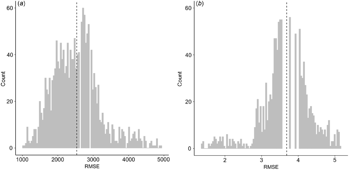
The accuracy and precision of the existing APSIM-Wheat module for predicting grain yield and protein varied considerably between unique combinations of APSIM-Wheat cultivars and field genotypes (Fig. 2). For grain yield, across all pair-wise comparisons, the relationships observed for RMSE ranged from 1040 to 4900 kg/ha and nRMSE from 16% to 68%. The RMSE of protein varied from 1.4% to 5.1% and the nRMSE varied from 17% to 74%.
Distribution of root-mean-square-errors (RMSE) between all combinations of APSIM-Wheat cultivars and field genotypes tested in the analysis for (a) grain yield and (b) grain protein. Dashed line shows the mean value.
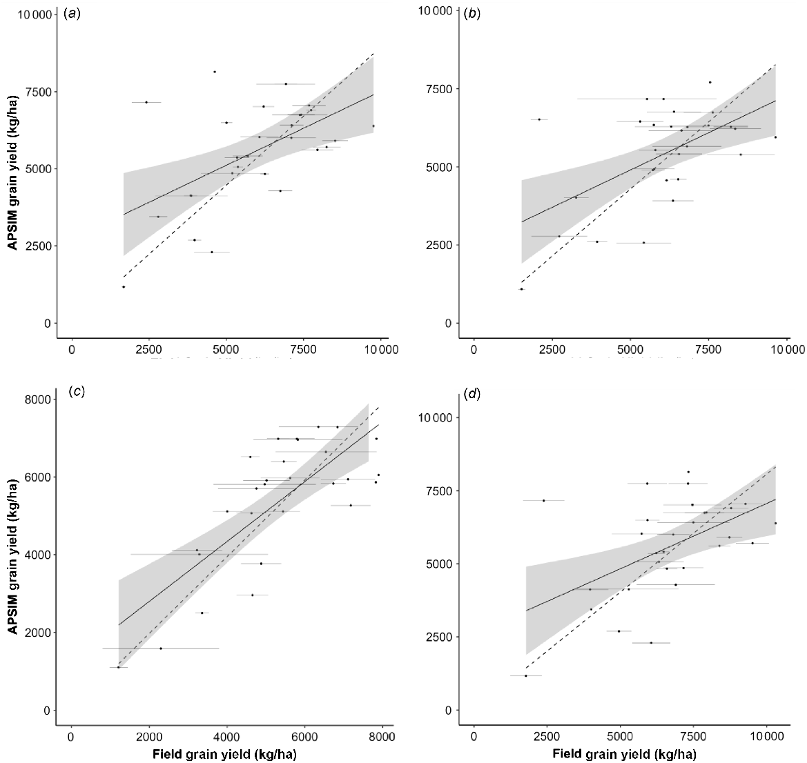
In terms of grain yield, the best linear relationships between the simulated and field data for SY Cal Rojo (UC1478) and SY Blanca Grande 515 (UC1657) are presented in Fig. 3a, b. In both cases, the nRMSE was >20%, with multiple outliers, and the linear fit over-predicted lower yielding environments and under-predicted high-yielding environments. Across all pairwise combinations of APSIM cultivars and field genotypes, WB Joaquin Oro (UC1728) had one of the lowest values of RMSE for yield (Fig. 3c). There were few apparent outliers, and the fit was close to 1:1, despite over-prediction in lower yielding environments. The genotype LCS Atomo (UC1723) had the highest yields of all genotypes tested in the multi-environment trials and was therefore specifically examined. The best model fit for this genotype was relatively poor (Fig. 3d). The relationships between simulated and field data for grain protein content were considered poor by all metrics, the best fit being r2 = 0.35, and are not presented.
Relationships between grain yields from field and simulated genotypes: (a) SY Cal Rojo (UC1478) and APSIM cultivar Gatton Hartog (RMSE = 1750, nRMSE = 22%, mean absolute error = 1300, r2 = 0.30, intercept = 2720, slope = 0.48); (b) SY Blanca Grande 515 (UC1657) and APSIM cultivar Gregory (RMSE = 1730, nRMSE = 21%, mean absolute error = 1346, r2 = 0.32, intercept = 2512, slope = 0.48); (c) WB Joaquin Oro (UC1728) and APSIM cultivar V2_P2 (RMSE = 1129, nRMSE = 17%, mean absolute error = 1000, r2 = 0.59, intercept = 1257, slope = 0.77); (d) LCS Atomo (UC1723) and Gatton Hartog (RMSE = 2084, nRMSE = 24%, mean absolute error = 1694, r2 = 0.27, intercept = 2599, slope = 0.44). Solid line shows the unconstrained linear relationship and dashed line the 1:1 relationship. Shading indicates the 95% confidence interval.
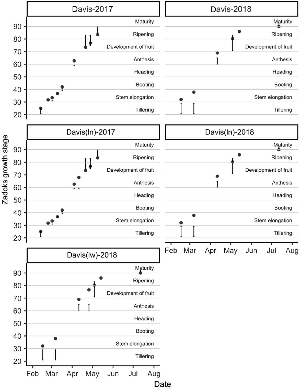
Performance of the APSIM-Wheat module for simulation of phenology
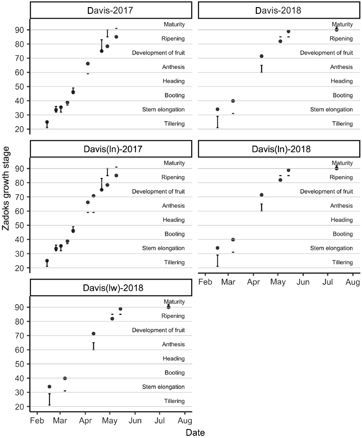
Figs 4 and 5 show the relationships between the observed field phenology of SY Cal Rojo (UC1478) and SY Blanca Grande 515 (UC1657), respectively, at the Davis location, and APSIM model predictions of phenology using the cultivars that gave the smallest RMSE of prediction for yield (as shown in Fig. 3). In all environments, the predicted time to all phenological stages between tillering and anthesis was slightly shorter than observed in the field, and was longer for late anthesis, early grain development, and grain maturation. The phenological data for WB Joaquin Oro (UC1728) and LCS Atomo (UC1723) showed a similar pattern but were available only for the Davis location in a single season, and at a lower temporal resolution, and are therefore not presented.
Relationship between observed phenology of field genotype SY Cal Rojo (UC1478) and predicted phenology of simulated APSIM cultivar Gatton Hartog (filled circles). Field observations span a range of phenology stages and are therefore represented as a value range (vertical lines). Observations were taken at the Davis location in the 2016–17 and 2017–18 seasons. ln, low-nitrogen managed-stress trial; lw, low-water managed-stress trials.
Relationship between observed phenology of field genotype SY Blanca Grande 515 (UC1657) and predicted phenology of APSIM cultivar Gregory (black circles). Field observations span a range of phenology stages and are therefore represented as a value range (vertical lines). Observations were taken at the Davis location in the 2016–17 and 2017–18 seasons. ln, low-nitrogen managed-stress trial; lw, low-water managed-stress trials.
Importance of management, environmental, and APSIM-Wheat parameters to simulation reliability
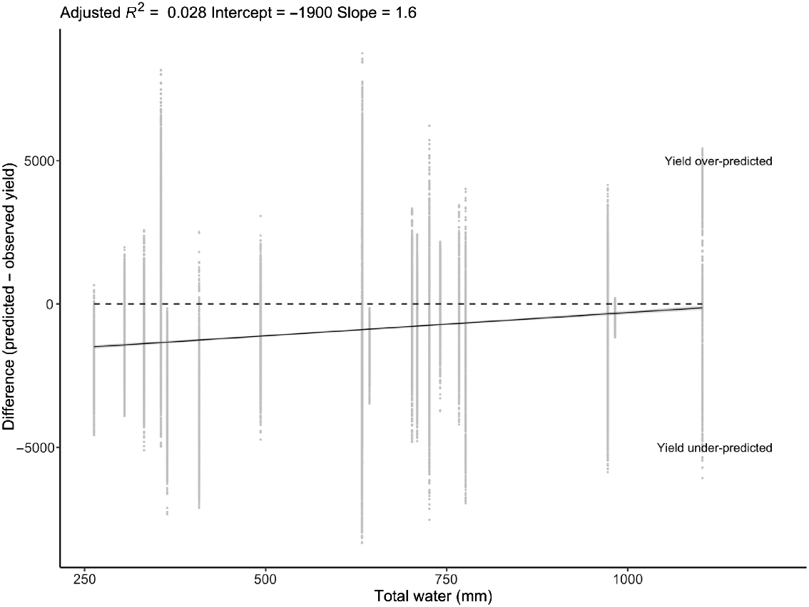
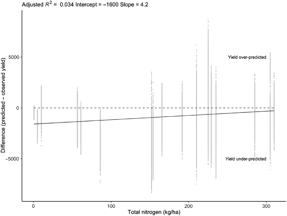
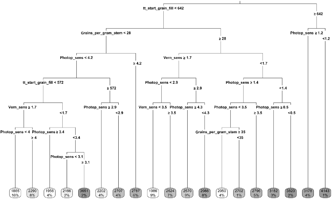
Water and nitrogen status of the locations was not strongly associated with model reliability; there was a trend whereby the yield at sites with lower water and nitrogen status was under-predicted, although the relationship was weak with large residual variation (Figs 6 and 7). CART analyses found thermal time to the start of grainfill and number of grains per stem weight were strong determinants of model reliability, as were vernalisation and photoperiod sensitivity (Fig. 8). Stepwise linear regression found all variables to have a significant impact on RMSE (Table 7), and similar to the CART analysis, thermal time to the start of grainfill and number of grains per stem weight had some of the largest impacts on model reliability. By contrast, vernalisation and photoperiod were not found to be strong predictors. The analysis was also performed using the coefficient of determination as the indicator of model reliability, but the results were the same as for RMSE between simulated and actual yield and protein data, and the results of the analysis are therefore not presented.
Relationship between total water (starting plant-available soil water, seasonal precipitation and irrigation) and the difference between predicted and observed yield across all locations and years. Dotted line shows no correlation between predictor and response (y = 0).
Relationship between total nitrogen (starting soil nitrogen and fertilisation) and the difference between predicted and observed yield across all locations and years. Dotted line shows no correlation between predictor and response (y = 0).
Classification and regression tree showing the importance of predictor variables to the RMSE of the linear relationship between all combinations of APSIM wheat cultivars and field genotypes for grain yield. See Tables 5 and 6 for a description of the values. Boxes along the bottom depict RMSE and the proportion of the dataset that falls in each division.
| Model | Beta | s.e. | t | Sign. | Lower | Upper | |
|---|---|---|---|---|---|---|---|
| tt_end_of_juvenile | −0.338 | 0.033 | −10.184 | 0 | −0.403 | −0.273 | |
| Max_grain_size | −0.219 | 0.039 | −5.653 | 0 | −0.295 | −0.143 | |
| Vern_sens | 0.099 | 0.023 | 4.28 | 0 | 0.054 | 0.144 | |
| Photop_sens | 0.106 | 0.024 | 4.439 | 0 | 0.059 | 0.152 | |
| tt_end_grain_fill | 0.108 | 0.025 | 4.239 | 0 | 0.058 | 0.157 | |
| tt_floral_initiation | 0.122 | 0.029 | 4.25 | 0 | 0.065 | 0.178 | |
| tt_flowering | 0.243 | 0.036 | 6.82 | 0 | 0.173 | 0.312 | |
| tt_start_grain_fill | 0.39 | 0.03 | 13.108 | 0 | 0.332 | 0.448 | |
| Grains_per_gram_stem | 0.427 | 0.038 | 11.181 | 0 | 0.352 | 0.502 |
Node senescence rate had only two unique values and was therefore removed from the analysis.
Observations of thermal time for phenological stages and model calibration
The thermal time spent in phenological stages was similar for both SY Cal Rojo (UC1478) and SY Blanca Grande 515 (UC1657), under conventional and managed-stress conditions in individual seasons. Comparison of thermal time spent in phenological stages with the equivalent parameter in the APSIM-Wheat module (Table 6) shows that the thermal times needed from sowing to the end of juvenile stage, from floral initiation to flowering, and to reach the anthesis stage were greater than for the APSIM cultivars, whereas thermal time needed from the beginning to end of grainfill was smaller.
Cultivar calibration
The APSIM base cultivar and New Zealand base cultivar were both reparameterised with thermal-time observations from SY Cal Rojo (UC1478) and SY Blanca Grande 515 (UC1657). However, like the unparameterised cultivars reported in Fig. 3, the reparameterised cultivars simulated WB Joaquin Oro (UC1728) most reliably (Table 8). The summary statistics show that the relationship between predicted and observed yield for the parameterised cultivars was worse than for the unparameterised model in Fig. 3.
| Parameterised APSIM cultivar | Field genotype | RMSE | nRMSE | r2 | Intercept | Slope | |
|---|---|---|---|---|---|---|---|
| Base | SY Blanca Grande 515 (UC1657) | 3011 | 37 | 0.06 | 3057 | 0.39 | |
| SY Cal Rojo (UC1478) | 2865 | 35 | 0.11 | 2433 | 0.50 | ||
| WB Joaquin Oro (UC1728) | 2437 | 37 | 0.24 | 886 | 0.82 | ||
| New Zealand base | SY Blanca Grande 515 (UC1657) | 2903 | 36 | 0.07 | 3358 | 0.41 | |
| SY Cal Rojo (UC1478) | 2765 | 34 | 0.13 | 2741 | 0.52 | ||
| WB Joaquin Oro (UC1728) | 2338 | 35 | 0.28 | 1041 | 0.87 |
Discussion
The performance of APSIM for simulation of wheat yield in California
Computer-based crop simulation models support agricultural research and production, but model calibration and testing requires field data that are often not available. The objective of this work was to use pre-existing data from state-wide field trials to evaluate the performance of the APSIM model (v7.10) for simulating wheat production in California and to identify future research needs for model validation and calibration. Given the large yield range and the diversity of environments, management methods and latitudes represented in the field data, we found that the APSIM model was capable of predicting relative grain yield responses for at least one field genotype. The accuracy of the relationship between predicted and reported field yields was comparable to other tests of the APSIM-Wheat module in environments where it has not been previously calibrated (Asseng et al. 2000; Farré et al. 2002; Zhao et al. 2014, 2020; Kouadio et al. 2015; Hussain et al. 2018).
Despite this, we do not consider the current APSIM-Wheat module to be accurate or precise enough to simulate wheat production scenarios in this environment, where greater specificity is required. The model could not reliably simulate high-yielding genotypes and was unable to reliably simulate grain protein content. The genotype that was simulated most reliably, WB Joaquin Oro (UC1728), was one of the lowest yielding of the advanced genotypes included in the California field trials, although it achieved some of the highest protein values (Nelsen et al. 2018, 2019). The usefulness of the current APSIM model for the Californian wheat industry is therefore limited, and it will require further calibration and validation.
Reasons for the performance of APSIM-wheat in California
The poor performance of APSIM for simulating wheat production in California is surprising given the environmental similarities between the region and southern Australia, where the model has been calibrated and extensively validated. The uncalibrated APSIM model has also previously been found to simulate canola production reliably in the same region (George and Kaffka 2017). Inaccuracies in crop simulation modelling result from both parameter sensitivity and parameterisation error (He et al. 2015).
Correct calibration of APSIM relies on genetic parameters that accurately represent the crop genotype being simulated (Ceglar et al. 2011; Zhao et al. 2014; Casadebaig et al. 2016; Harris et al. 2016; Meier et al. 2020). As would be expected, the performance of APSIM for simulating wheat in California was shown to vary considerably depending on the choice of APSIM cultivar and the field genotype with which it was compared. Analyses of the importance of variables for model reliability, observation of field phenology, and initial thermal-time estimates all suggest that the parameterisation of APSIM cultivars does not currently represent the Californian genotypes well. APSIM was able to approximate the phenology of field genotypes SY Cal Rojo (UC1478), SY Blanca Grande 515 (UC1657) and LCS Atomo (UC 1723) despite the yields of these genotypes not being simulated reliably. By contrast, the phenology of WB Joaquin Oro (UC1728) was not simulated as reliably, despite the yield of this genotype being simulated more reliably than that of other genotypes.
Several phenology and grain parameters are influencing the outcome of the simulation. Parameterisation of the model using field observations of thermal time did not lead to improvements in yield simulations. Therefore, fieldwork is necessary to develop a better understanding of these phenology and grain parameters in Californian varieties. Most wheat genotypes in California are considered to have a low sensitivity to vernalisation and are photoperiod-insensitive (Dubcovsky et al. 2006). However, Ottman et al. (2013) demonstrated that consideration of photoperiod alongside thermal time improves predictions of flowering date in autumn/fall-planted spring wheat cultivars in the south-west of USA. Our findings also suggest that photoperiod and vernalisation sensitivity are important predictors and should also be investigated in more detail.
All efforts were made to parameterise the model to accurately reflect environmental and management conditions at the locations using reported data, but there are reasons to believe the management and environmental data for some locations are not accurate. The RMSE of prediction of yield of WB Joaquin Oro (UC 1728) was also comparable to the reported single-site standard deviation from the field data for the genotype (George et al. 2017; Nelsen et al. 2018, 2019), illustrating the sensitivity of yield to environmental factors within field sites not being captured by the simulation, along with the potential for imprecisions in reported management and environmental data at field sites.
Datasets from state-wide multi-environment trials, which are often long-running, geographically extensive, agro-environmentally diverse, and publicly available, are resources for understanding the impacts of management and environmental data on crop production (e.g. George and Lundy 2019; Barrett-Lennard et al. 2024). Within resourcing limits, the California Small Grains Program collects comprehensive data regarding crops and test locations (George et al. 2017; Nelsen et al. 2018, 2019), but our study shows such datasets may still have limitations due to insufficient resolution or completeness. Well-conducted multi-environment trials are essential for effective plant breeding and agronomy (Yan 2014) and will continue to be routine in many regions of the world. Existing multi-environment trials should therefore be leveraged to generate data that can be applied to analytics and modelling (Keating 2020; Pasquel et al. 2022). This will increase the long-term value of these programs.
Conclusions and future work: improvement of the APSIM-Wheat module for California
The current APSIM-Wheat module calibration is not able to simulate wheat production reliably under Californian conditions. Models such as APSIM will continue to be important tools for agricultural research and management (Chenu et al. 2017; Keating 2020), and increasing the accuracy and precision of the APSIM-Wheat module for Californian conditions will provide a tool to support and complement existing agricultural research. Our study finds that data needed for model calibration are not currently available. Future work should therefore prioritise higher resolution observations of phenology, sensitivity to photoperiod and vernalisation, and grain characteristics, as well as canopy development and senescence (Zheng et al. 2015; Brown et al. 2018). Seasonal biomass accumulation and soil-water dynamics would also be valuable (Asseng et al. 1998) and assist in improving simulations.
Data availability
The data that support this study are available in Dryad at: https://datadryad.org/stash/share/YpQMK9qqFHhtUTrbQ0rndYGMt_ekh1Hk4Zd4IK7vsLI.
Acknowledgements
The following people and organisations are thanked: The Australia Awards Scholarship for supporting Mr Helio de Jesus Pedro Cuamba; Dr Imma Farré and Dr Lindsay Bell for their advice regarding APSIM; Dr Ayalsew Zerihun and Dr Raphael Viscarra Rossel for their advice regarding data analysis; Dr Jorge Dubcovsky for providing information regarding wheat genotypes in California; the staff and students at the University of California Small Grains Program. In addition, the California Wheat Commission, the California Crop Improvement Association, and the University of California Division of Agriculture and Natural Resources are thanked for making field data publicly available.
References
Ahmed M, Akram MN, Asim M, Aslam M, Hassan F-U, Higgins S, et al. (2016) Calibration and validation of APSIM-wheat and CERES-wheat for spring wheat under rainfed conditions: models evaluation and application. Computers and Electronics in Agriculture 123, 384-401.
| Crossref | Google Scholar |
Archontoulis SV, Miguez FE, Moore KJ (2014a) Evaluating APSIM maize, soil water, soil nitrogen, manure, and soil temperature modules in the Midwestern United States. Agronomy Journal 106, 1025-1040.
| Crossref | Google Scholar |
Archontoulis SV, Miguez FE, Moore KJ (2014b) A methodology and an optimization tool to calibrate phenology of short-day species included in the APSIM PLANT model: application to soybean. Environmental Modelling & Software 62, 465-477.
| Crossref | Google Scholar |
Asseng S, Keating BA, Fillery IRP, Gregory PJ, Bowden JW, Turner NC, et al. (1998) Performance of the APSIM-wheat model in Western Australia. Field Crops Research 57, 163-179.
| Crossref | Google Scholar |
Asseng S, van Keulen H, Stol W (2000) Performance and application of the APSIM Nwheat model in the Netherlands. European Journal of Agronomy 12, 37-54.
| Crossref | Google Scholar |
Asseng S, Turner NC, Keating BA (2001) Analysis of water-and nitrogen-use efficiency of wheat in a Mediterranean climate. Plant and Soil 233, 127-143.
| Crossref | Google Scholar |
Balboa GR, Archontoulis SV, Salvagiotti F, Garcia FO, Stewart WM, Francisco E, et al. (2019) A systems-level yield gap assessment of maize-soybean rotation under high-and low-management inputs in the Western US Corn Belt using APSIM. Agricultural Systems 174, 145-154.
| Crossref | Google Scholar |
Barrett-Lennard EG, D’Antuono M, George N, Holmes KW, Ward PR (2024) Rainfall, reference evapotranspiration and fertiliser application are the main variables affecting crop yield in National Variety Trials under rainfed conditions across southern Australia. Crop & Pasture Science In press.
| Google Scholar |
Blunden J, Boyer T (2021) A look at 2020: takeaway points from the state of the climate. Bulletin of the American Meteorological Society 102, 756-768.
| Crossref | Google Scholar |
Brown H, Huth N, Holzworth D (2018) Crop model improvement in APSIM: using wheat as a case study. European Journal of Agronomy 100, 141-150.
| Crossref | Google Scholar |
California Soil Resources Lab (2020) Streaming soil survey data. California Soil Resources Laboratory, University of California, Davis. Available at http://casoilresource.lawr.ucdavis.edu/drupal/node/538
Casadebaig P, Zheng B, Chapman S, Huth N, Faivre R, Chenu K (2016) Assessment of the potential impacts of wheat plant traits across environments by combining crop modeling and global sensitivity analysis. PLoS ONE 11, e0146385.
| Crossref | Google Scholar | PubMed |
Ceglar A, Črepinšek Z, Kajfež-Bogataj L, Pogačar T (2011) The simulation of phenological development in dynamic crop model: the Bayesian comparison of different methods. Agricultural and Forest Meteorology 151, 101-115.
| Crossref | Google Scholar |
Chenu K, Porter JR, Martre P, Basso B, Chapman SC, Ewert F, et al. (2017) Contribution of crop models to adaptation in wheat. Trends in Plant Science 22, 472-490.
| Crossref | Google Scholar | PubMed |
Chenu K, Van Oosterom EJ, McLean G, Deifel KS, Fletcher A, Geetika G, et al. (2018) Integrating modelling and phenotyping approaches to identify and screen complex traits: transpiration efficiency in cereals. Journal of Experimental Botany 69, 3181-3194.
| Crossref | Google Scholar | PubMed |
CIMIS (2020) California irrigation management information system. California Department of Water Resources Office of Water Use Efficiency, Sacramento, CA. Available at http://wwwcimis.water.ca.gov/cimis/data.jsp
Dubcovsky J (2020) Distinguished Professor, Department of Plant Sciences, the University of California, Davis. (Ed. NA George). Available at https://dubcovskylab.ucdavis.edu/home
Dubcovsky J, Loukoianov A, Fu D, Valarik M, Sanchez A, Yan L (2006) Effect of photoperiod on the regulation of wheat vernalization genes VRN1 and VRN2. Plant Molecular Biology 60, 469-480.
| Crossref | Google Scholar | PubMed |
Farré I, Robertson MJ, Walton GH, Asseng S (2002) Simulating phenology and yield response of canola to sowing date in Western Australia using the APSIM model. Australian Journal of Agricultural Research 53, 1155-1164.
| Crossref | Google Scholar |
George N, Kaffka S (2017) Canola as a new crop for California: a simulation study. Agronomy Journal 109, 496-509.
| Crossref | Google Scholar |
George N, Lundy M (2019) Quantifying genotype × environment effects in long-term common wheat yield trials from an agroecologically diverse production region. Crop Science 59, 1960-1972.
| Crossref | Google Scholar |
George N, Thompson SE, Hollingsworth J, Orloff S, Kaffka S (2018) Measurement and simulation of water-use by canola and camelina under cool-season conditions in California. Agricultural Water Management 196, 15-23.
| Crossref | Google Scholar |
Hammer GL, McLean G, van Oosterom E, Chapman S, Zheng B, Wu A, et al. (2020) Designing crops for adaptation to the drought and high-temperature risks anticipated in future climates. Crop Science 60, 605-621.
| Crossref | Google Scholar |
Harris F, Martin P, Eagles H (2016) Understanding wheat phenology: flowering response to sowing time. GRDC Grains Research Update, Wagga, NSW. Available at https://grdc.com.au/Research-and-Development/GRDC-Update-Papers/2016/02/Understanding-wheat-phenologyflowering-response-to-sowing-time
He L, Zhao G, Jin N, Zhuang W, Yu Q (2015) Global sensitivity analysis of APSIM-Wheat parameters in different climate zones and yield levels. Transactions of the Chinese Society of Agricultural Engineering 31, 148-157.
| Crossref | Google Scholar |
Hebbali A (2020) olsrr: tools for building OLS regression models. R package version 0.5.3. Available at https://CRAN.R-project.org/package=olsrr
Hochman Z, van Rees H, Carberry PS, Hunt JR, McCown RL, Gartmann A, et al. (2009a) Re-inventing model-based decision support with Australian dryland farmers. 4. Yield Prophet® helps farmers monitor and manage crops in a variable climate. Crop & Pasture Science 60, 1057-1070.
| Crossref | Google Scholar |
Hochman Z, Holzworth D, Hunt JR (2009b) Potential to improve on-farm wheat yield and WUE in Australia. Crop & Pasture Science 60, 708-716.
| Crossref | Google Scholar |
Holzworth DP, Huth NI, deVoil PG, Zurcher EJ, Herrmann NI, McLean G, et al. (2014) APSIM – evolution towards a new generation of agricultural systems simulation. Environmental Modelling & Software 62, 327-350.
| Crossref | Google Scholar |
Holzworth D, Huth NI, Fainges J, Brown H, Zurcher E, Cichota R, et al. (2018) APSIM next generation: overcoming challenges in modernising a farming systems model. Environmental Modelling & Software 103, 43-51.
| Crossref | Google Scholar |
Hussain J, Khaliq T, Ahmad A, Akhtar J (2018) Performance of four crop model for simulations of wheat phenology, leaf growth, biomass and yield across planting dates. PLoS ONE 13, e0197546.
| Crossref | Google Scholar | PubMed |
Keating BA (2020) Crop, soil and farm systems models – science, engineering or snake oil revisited. Agricultural Systems 184, 102903.
| Crossref | Google Scholar |
Keating BA, Carberry PS, Hammer GL, Probert ME, Robertson MJ, Holzworth D, et al. (2003) An overview of APSIM, a model designed for farming systems simulation. European Journal of Agronomy 18, 267-288.
| Crossref | Google Scholar |
Kotir J, Bell L, Kirkegaard J, Whish J, Atkins KA (2020) Farm resource use as influenced by diverse cropping systems in the Australian Northern cropping zone. In ‘The 64th Annual Conference of the Australasian Agricultural and Resource Economics Society (AARES)’. Perth, Western Australia, 12–14 February 2020. p. 5. (Australian Agricultural and Resource Economics Society)
Kouadio L, Newlands N, Potgieter A, McLean G, Hill H (2015) Exploring the potential impacts of climate variability on spring wheat yield with the APSIM decision support tool. Agricultural Sciences 6, 686-698.
| Crossref | Google Scholar |
Lawes RA, Oliver YM, Huth NI (2019) Optimal nitrogen rate can be predicted using average yield and estimates of soil water and leaf nitrogen with infield experimentation. Agronomy Journal 111, 1155-1164.
| Crossref | Google Scholar |
Meier E, Lilley J, Kirkegaard J, Whish J, McBeath T (2020) Management practices that maximise gross margins in Australian canola (Brassica napus L.). Field Crops Research 252, 107803.
| Crossref | Google Scholar |
Muller B, Martre P (2019) Plant and crop simulation models: powerful tools to link physiology, genetics, and phenomics. Journal of Experimental Botany 70(9), 2339-2344.
| Crossref | Google Scholar |
Ottman MJ, Anthony Hunt L, White JW (2013) Photoperiod and vernalization effect on anthesis date in winter-sown spring wheat regions. Agronomy Journal 105, 1017-1025.
| Crossref | Google Scholar |
Pasquel D, Roux S, Richetti J, Cammarano D, Tisseyre B, Taylor JA (2022) A review of methods to evaluate crop model performance at multiple and changing spatial scales. Precision Agriculture 23, 1489-1513.
| Crossref | Google Scholar |
Pathak TB, Maskey ML, Dahlberg JA, Kearns F, Bali KM, Zaccaria D (2018) Climate change trends and impacts on California agriculture: a detailed review. Agronomy 8, 25.
| Crossref | Google Scholar |
Peake AS, Huth NI, Carberry PS, Raine SR, Smith RJ (2014) Quantifying potential yield and lodging-related yield gaps for irrigated spring wheat in sub-tropical Australia. Field Crops Research 158, 1-14.
| Crossref | Google Scholar |
Peel MC, Finlayson BL, Mcmahon TA (2007) Updated world map of the Köppen-Geiger climate classification. Hydrology and Earth System Sciences Discussions 4, 439-473.
| Crossref | Google Scholar |
R Core Team (2020) ‘R: a language and environment for statistical computing.’ (R Foundation for Statistical Computing: Vienna, Austria) Available at https://www.R-project.org/
Ramirez-Villegas J, Molero Milan A, Alexandrov N, Asseng S, Challinor AJ, Crossa J, et al. (2020) CGIAR modeling approaches for resource-constrained scenarios: I. Accelerating crop breeding for a changing climate. Crop Science 60, 547-567.
| Crossref | Google Scholar |
Reardon-Smith K, Mushtaq S, Farley HS, Cliffe N, Stone RC, Ostini J, et al. (2015) Virtual discussions to support climate risk decision making on farms. Journal of Economic and Social Policy 17, 7-1-7-12.
| Google Scholar |
Robertson MJ, Rebetzke GJ, Norton RM (2015) Assessing the place and role of crop simulation modelling in Australia. Crop & Pasture Science 66, 877-893.
| Crossref | Google Scholar |
Sadras VO (2020) On water-use efficiency, boundary functions, and yield gaps: French and Schultz insight and legacy. Crop Science 60, 2187-2191.
| Crossref | Google Scholar |
Therneau T, Atkinson B (2019) rpart: recursive partitioning and regression trees. R package version 4.1-15. Available at https://CRAN.R-project.org/package=rpart
USDA NASS (2020) United States Department of Agriculture National Agricultural Statistics Service. Washington, DC. Available at http://www.nass.usda.gov/
Williams AP, Cook BI, Smerdon JE (2022) Rapid intensification of the emerging southwestern North American megadrought in 2020–2021. Nature Climate Change 12, 232-234.
| Crossref | Google Scholar |
Ye Z, Qiu X, Chen J, Cammarano D, Ge Z, Ruane AC, et al. (2020) Impacts of 1.5° C and 2.0° C global warming above pre-industrial on potential winter wheat production of China. European Journal of Agronomy 120, 126149.
| Crossref | Google Scholar |
Yunusa IAM, Bellotti WD, Moore AD, Probert ME, Baldock JA, Miyan SM (2004) An exploratory evaluation of APSIM to simulate growth and yield processes for winter cereals in rotation systems in South Australia. Australian Journal of Experimental Agriculture 44, 787-800.
| Crossref | Google Scholar |
Zadoks JC, Chang TT, Konzak CF (1974) A decimal code for the growth stages of cereals. Weed Research 14(6), 415-421.
| Crossref | Google Scholar |
Zambrano-Bigiarini M (2020) hydroGOF: goodness-of-fit functions for comparison of simulated and observed hydrological time series. R package version 0.4-0. Available at https://github.com/hzambran/hydroGOF
Zhao G, Bryan BA, Song X (2014) Sensitivity and uncertainty analysis of the APSIM-wheat model: interactions between cultivar, environmental, and management parameters. Ecological Modelling 279, 1-11.
| Crossref | Google Scholar |
Zhao C, Liu B, Xiao L, Hoogenboom G, Boote KJ, Kassie BT, et al. (2019) A SIMPLE crop model. European Journal of Agronomy 104, 97-106.
| Crossref | Google Scholar |
Zhao P, Zhou Y, Li F, Ling X, Deng N, Peng S, et al. (2020) The adaptability of APSIM-wheat model in the middle and lower reaches of the Yangtze River Plain of China: a case study of winter wheat in Hubei Province. Agronomy 10, 981.
| Crossref | Google Scholar |
Zheng B, Chenu K, Fernanda Dreccer M, Chapman SC (2012) Breeding for the future: what are the potential impacts of future frost and heat events on sowing and flowering time requirements for Australian bread wheat (Triticum aestivium) varieties? Global Change Biology 18, 2899-2914.
| Crossref | Google Scholar | PubMed |
Zheng B, Chenu K, Doherty A, Chapman S (2015) The APSIM-wheat module (7.5R3008). Available at https://www.apsim.info/wp-content/uploads/2019/09/WheatDocumentation.pdf