

Estimating post-fire debris-flow hazards prior to wildfire using a statistical analysis of historical distributions of fire severity from remote sensing data
Dennis M. Staley A D , Anne C. Tillery B , Jason W. Kean A , Luke A. McGuire C , Hannah E. Pauling A , Francis K. Rengers A and Joel B. Smith AA U.S. Geological Survey, Landslide Hazards Program, Golden, CO 80422, USA.
B U.S. Geological Survey, New Mexico Water Science Center, Albuquerque, NM 87113, USA.
C University of Arizona, Department of Geosciences, Tucson, AZ 85721, USA.
D Corresponding author. Email: dstaley@usgs.gov
International Journal of Wildland Fire 27(9) 595-608 https://doi.org/10.1071/WF17122
Submitted: 16 August 2017 Accepted: 6 August 2018 Published: 24 August 2018
Journal Compilation © IAWF 2018 Open Access CC BY-NC-ND
Abstract
Following wildfire, mountainous areas of the western United States are susceptible to debris flow during intense rainfall. Convective storms that can generate debris flows in recently burned areas may occur during or immediately after the wildfire, leaving insufficient time for development and implementation of risk mitigation strategies. We present a method for estimating post-fire debris-flow hazards before wildfire using historical data to define the range of potential fire severities for a given location based on the statistical distribution of severity metrics obtained from remote sensing. Estimates of debris-flow likelihood, magnitude and triggering rainfall threshold based on the statistically simulated fire severity data provide hazard predictions consistent with those calculated from fire severity data collected after wildfire. Simulated fire severity data also produce hazard estimates that replicate observed debris-flow occurrence, rainfall conditions and magnitude at a monitored site in the San Gabriel Mountains of southern California. Future applications of this method should rely on a range of potential fire severity scenarios for improved pre-fire estimates of debris-flow hazard. The method presented here is also applicable to modelling other post-fire hazards, such as flooding and erosion risk, and for quantifying trends in observed fire severity in a changing climate.
Additional keywords: hazard assessment, mass movement, risk.
Introduction
Recently burned areas in the western United States are susceptible to debris flows even without antecedent rainfall, as post-fire debris flows have been initiated during the first few minutes of the first significant rainstorm following wildfire (Wells 1987; Cannon et al. 2008; Kean et al. 2011). In the western United States, wildfire may be coincident with intense convective storms that produce rainfall intensities sufficient for generation of debris flows. In such cases, there is limited time for public officials to develop and implement potentially costly and time-consuming risk-mitigation or risk-reduction strategies and emergency management plans that address post-fire debris flow hazards.
Currently, predictive models of debris-flow likelihood, magnitude and triggering rainfall conditions have been developed to reduce risk from post-fire debris-flow hazards (Cannon et al. 2008; Cannon et al. 2010; Staley et al. 2016, 2017; USGS 2018a). These models combine data related to the severity of wildfire, the steepness of the burned terrain and the physical properties of the soils to estimate post-fire debris-flow hazards in response to a range of rainfall intensities (Table 1). The predictive equations require a priori information about the severity of the wildfire (Gartner et al. 2014; Staley et al. 2016, 2017), including the differenced Normalized Burn Ratio (dNBR) obtained from remote sensing techniques (French et al. 2008), and a map of field-validated soil burn severity (Key and Benson 2006; Parson et al. 2010). However, direct prediction of fire severity and associated metrics (i.e. dNBR and soil burn severity) and potential debris-flow hazards for future wildfires is an infrequently explored topic in the scientific literature (Tillery et al. 2014; Haas et al. 2016; Tillery and Haas 2016).

|
The natural patterns of fire severity that result from wildfire are a result of a complex interaction between weather conditions, vegetation characteristics, fuel conditions and topography (Rollins et al. 2002). ‘Fire severity’ is a general term used to describe the surface and subsurface changes in organic matter composition that result from wildfire (Keeley 2009), frequently estimated using dNBR. ‘Soil burn severity’ is a more specific term used to describe the relative change in soil properties (organic matter content, soil strength, infiltration capacity) that results from wildfire, as estimated in the field (Parson et al. 2010).
Several studies have attempted to predict fire severity before wildfire. Fire simulation models, such as FlamMap (Finney 2006) model fire behaviour (i.e. growth rate, shape, flame length, crown fire activity, etc.). The FlamMap output represents a single realisation of a potential fire, and not the potential range of behaviours. FSim (Finney et al. 2011) models conditional flame length and fire intensity, which can be used as a proxy for fire severity. Holden et al. (2009) developed an empirical model for predicting the probability of severe fire occurrence from topographic variables. However, the authors conclude that model predictions are unlikely to accurately predict future burn severity at specific locations within their study area in Arizona, and are unlikely to be applicable for other regions. The FIRESEV project (Keane et al. 2013) expands on the approach of Holden et al. (2009) to predict the potential for high-severity fire throughout the western United States. However, FlamMap, FSim and FIRESEV do not explicitly produce quantitative predictions of dNBR or soil burn severity required for assessment of post-fire debris-flow hazards. Additionally, the models only predict the probability of a high-severity fire, and does not explicitly predict soil burn severity or dNBR.
Few efforts to estimate potential debris-flow hazards before the occurrence of fire (Stevens et al. 2011; Lancaster et al. 2014; Tillery et al. 2014; Haas et al. 2016; Tillery and Haas 2016) have been attempted. Stevens et al. (2011) used the presence of vegetation cover as an indicator of fire severity. Here, the authors assumed a ‘worst-case’ scenario, where any vegetation cover defined as shrub or forest type, as identified by the National Land Cover Database (Homer et al. 2007), was assumed to burn at high or moderate severity. Tillery et al. (2014) describe an approach for pre-fire prediction of debris-flow hazards by combining fire simulation models (Finney 2006; Finney et al. 2011) with an older generation of models of debris-flow hazard estimation (Cannon et al. 2010) to estimate the potential likelihood and volume of post-fire debris flows in New Mexico. Although this approach, also used by Haas et al. (2016) and Tillery and Haas (2016), provides useful information such as burn probabilities, it is limited in its applicability for debris-flow prediction using current modelling equations for two reasons. First, the fire simulation models used in these analyses are labour-intensive and require a thorough understanding of wildfire processes and associated variables. Second, the fire behaviour models do not directly predict dNBR values, which are an independent variable in the models used to estimate post-fire debris-flow likelihood (Staley et al. 2016), magnitude (Gartner et al. 2014) and rainfall intensity-duration thresholds (Staley et al. 2017) (Table 1). Instead, Tillery et al. (2014) used crown fire potential as a proxy for burn severity. Lancaster et al. (2014) relied on a scenario-based approach for characterising fire extent and soil burn severity that assumed varying proportions of high and moderate soil burn severity (i.e. 25, 50 and 100% of the upslope area) to estimate post-fire debris-flow likelihood, volume and combined hazard for 20 watersheds in southern California.
Although the approaches of Stevens et al. (2011) and Lancaster et al. (2014) are conceptually and computationally much simpler than the method of Tillery et al. (2014), none of the reviewed methods directly predict dNBR and, therefore, they are of limited applicability when using the current generation of equations for estimating post-fire debris-flow likelihood, magnitude and rainfall intensity-duration thresholds (Table 1). In addition, the methods of Stevens et al. (2011), Lancaster et al. (2014), Tillery et al. (2014), Tillery and Haas (2016), or Haas et al. (2016) were not tested for accuracy against actual post-fire data, a step that is critical to ensure that the predictions provided by simulations accurately represent potential debris-flow hazards for the modelled areas. Therefore, there is a current research need to model fire severity using an approach that can be combined with existing statistical models for estimating debris-flow likelihood, magnitude and rainfall intensity-duration threshold and verified using existing debris-flow occurrence and magnitude data.
In what follows, we present an alternative approach that is simple in application, requires limited and publicly available input data, produces a dNBR output, and is tested for accuracy using eight test datasets and a case study from the San Gabriel Mountains of southern California. We describe a statistical method for predicting post-fire debris-flow hazards before wildfire occurrence, which can be used by public officials such as land managers and emergency coordinators to answer the following question: ‘Should a fire occur in this watershed, what will be the expected range of debris-flow likelihood, magnitude and rainfall intensity-duration thresholds?’ We do not attempt to directly predict natural or simulated geographic patterns of fire severity or the probability of fire occurrence in a specific location. Instead, we focus our efforts on attempting to better define the historical distribution of fire severity for individual vegetation types. We use this information to constrain the statistical range of potential dNBR and soil burn severity for a given location along a stream channel, which can then be used to estimate debris-flow hazards in unburned locations. Specifically, we demonstrate the application of the method to an unburned area in the Wasatch Mountains above Salt Lake City, Utah, using three potential fire scenarios: a moderately frequent moderate-severity fire; a moderately infrequent higher-severity fire; and an infrequent fire with very high severity.
Methods
We hypothesise that we can adequately simulate fire severity (dNBR) and soil burn severity to accurately depict post-fire debris-flow hazards using a statistical approach. This methodology assumes that in the near term, wildfires will have a similar distribution of fire severity (measured using dNBR) to past wildfires. To test our hypothesis, we calculate a statistical distribution of dNBR for each vegetation type within a large calibration dataset of historically burned areas. We then define the historical frequency of dNBR values using a cumulative distribution function (CDF) for different types of vegetation and define soil burn severity classes from the simulated dNBR. The derived dNBR and soil burn severity data are entered into the post-fire debris-flow hazard assessment equations to estimate the potential likelihood (Staley et al. 2016), magnitude (Gartner et al. 2014) and 15-min rainfall intensity-duration threshold (Staley et al. 2017) for eight recently burned areas not included in the calibration dataset. We test the predictive accuracy of the proposed methodology by comparing the results of the simulated models with those calculated using the observed post-fire burn severity data for these eight test areas. A flow chart depicting the processing steps can be found in Fig. S1 (available as supplementary material to this paper online).
We relied on historical data characterising fire severity to derive a statistical distribution of dNBR for each class of LandFire Existing Vegetation Type (EVT) (Rollins 2009; LandFire 2017) in the calibration dataset. Testing our hypothesis relied on five methodological components. First, we analysed fire severity information derived from remote sensing data (Eidenshink et al. 2007; MTBS 2017). Second, we defined the historical distribution of dNBR values and burn severity for fires that occurred between 2001 and 2014 in each of the study regions. Third, we simulated fire severity data for the eight recently burned areas composing the test dataset (Table 1). Fourth, we compared estimates of debris-flow hazard based on simulated and observed fire severity data for the eight recently burned areas in the test dataset. Fifth, we compared simulated and post-fire estimates of debris-flow likelihood, magnitude and rainfall intensity-duration threshold with debris-flow occurrence and magnitude data obtained at a monitoring site in the San Gabriel Mountains of southern California during the winter of 2016–17. We then present an example of a scenario-based pre-fire assessment of debris-flow hazards for a portion of the Wasatch Front above suburban Salt Lake City, Utah, that has not been subject to wildfire in the past several decades.
Study areas
The Monitoring Trends in Burn Severity (MTBS) database (Eidenshink et al. 2007; MTBS 2017) was used to define the statistical distribution of fire severity for all EVT classes within every documented fire ≥4 km2 (1000 acres) occurring in the western United States from 1 January 2001 through 31 December 2014.1 In total, 3163 individual burn areas compose the calibration set, which comprised 176 621 km2 of burned terrain and 282 unique EVT classes. We then tested the methodology for pre-fire estimation of post-fire debris-flow hazards for eight burn areas in four regions (Table 2) that covered a range of physiographic conditions and a diversity of vegetation types. The four regions consisted of (1) the San Gabriel and San Bernardino Mountains of southern California (the 2016 San Gabriel Complex and Blue Cut fires); (2) the southern Cascade Mountains of northern California, including the Siskiyou and Salmon Mountains (the 2016 Gap and Pony fires); (3) the central Rocky Mountains of southern Colorado, including the eastern San Juan, Sangre de Cristo and Wet Mountains (2016 Hayden Pass and Junkins fires); and (4) the Chelan Mountains of the Cascade Range in central Washington near Lake Chelan (the 2015 Wolverine and First Creek fires) (Fig. 1).

|

|
Hydrological and meteorological data were collected at the Las Lomas debris-flow monitoring site in the San Gabriel Complex during the winter of 2016–17 (Fig. 2) using methods previously described by Kean et al. (2011). Monitoring data from this location recorded flow stage and rainfall rates for 29 storm events, 5 of which generated debris flows: 16 December 2016, 23 December 2016, 11 January 2017, 20 January 2017 and 17 February 2017. Video footage of a debris flow at the Las Lomas monitoring site on 20 January 2017 can be found online at the USGS Landslide Hazards Program post-fire debris-flow hazards website (USGS 2018b). Volumetric data for three debris-flow events were obtained from an analysis of the observed debris levels in the Las Lomas sediment retention basin following the methods described by Gartner et al. (2014).

|
Quantifying fire severity from remote sensing data
The severity of wildfire influences the amount that vegetation cover is reduced and the magnitude of changes in the chemical and physical properties of soils, which in turn alter surface and near-surface hydrology (Shakesby and Doerr 2006; Keeley 2009). The net effect of these changes contributes to increases in the susceptibility of recently burned watersheds to debris flow (Cannon 2001). Data derived from remote sensing techniques, including dNBR and soil burn severity, are frequently used to characterise these wildfire-induced changes. In the present study, we utilise the following remote sensing products: dNBR, Burned Area Reflectance Classification with four classes (BARC4), and soil burn severity from the MTBS website (MTBS 2017) and the Burned Area Emergency Response (BAER) imagery support website (USFS 2018). Detailed discussion of the methods for deriving these products is outside the scope of the present paper, but readers seeking additional information on these products should seek out the primary sources (Key and Benson 2006; Roy et al. 2006; Eidenshink et al. 2007; Parson et al. 2010; Kolden et al. 2015; MTBS 2017).
Quantifying the historical distributions of fire severity
Recently, vegetation type has been used as context to better understand historical patterns and trends of fire severity (Picotte et al. 2016), because the magnitude of spectral changes that occur in response to wildfire varies with vegetation type. Thus, similar dNBR values in different vegetation types do not necessarily reflect a similar degree of fire severity (Eidenshink et al. 2007; Kolden et al. 2015). For example, grasslands are typically entirely consumed during wildfire, resulting in a very high dNBR value in spite of observed low burn severity (Roy et al. 2006).
We address this dissimilarity in spectral response by using LandFire data (Rollins 2009; LandFire 2017) to analyse this historical distribution of dNBR within each EVT for all fires in the calibration dataset. The LandFire dataset is periodically updated to incorporate changes in landcover associated with disturbance, such as wildfire. The present analysis utilises updates from 2001 (version 105), 2008 (version 110), 2010 (version 120), 2012 (version 130) and 2014 (version 140) (LandFire 2017) to characterise EVT for each analysed burn area. The EVT version that was published in closest temporal proximity and before each fire was used for the calibration dataset. For example, a fire that burned in 2009 utilises the 2008 (version 110) dataset to characterise pre-fire EVT.
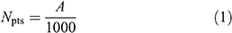
To define the historical distribution of dNBR values within each vegetation type, EVT and dNBR were randomly sampled within each of the 3163 burn areas, where the number of sample points (Npts) within the perimeter is a function of area burned (A, in m2):
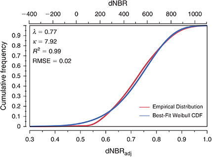
Sample points were selected in a stratified random process, where only pixels that were classified as having low, moderate or high burn severity were sampled in order to avoid the influence of unburned vegetation on the statistical distribution of dNBR, as recommended for any analysis of MTBS data in Kolden et al. (2015). From these data, we fitted a Weibull CDF to the sampled dNBR data for each vegetation type (Staley 2018). This flexible, two-parameter CDF has been demonstrated to accurately define the distribution of fire severity data in other recently burned areas (Lutz et al. 2011). The high R2 and low root-mean-square error (RMSE) values calculated during the analysis of the fitted distribution (Staley, 2018) add further support to the use of this distribution in the current analysis.
Calculation of the Weibull CDF requires that all data values be greater than zero. To meet that requirement, we rescaled the dNBR data (which ranged from −1000 to +1000) to an adjusted dNBR (dNBRadj) before fitting the CDF by using the following equation:

We then identified the Weibull CDF for every EVT class by calculating the best-fit  (shape parameter) and
  (scale parameter) for the CDF using the equation:

where Pd is the cumulative probability of a location of having a dNBRadj value less than or equal to the calculated value. An example of the Weibull CDF fit to dNBR sample data for the central and southern California Mixed Evergreen Woodland vegetation type (EVT group 3014) can be found in Fig. 3. Best-fit Weibull CDF parameters and statistical measures of goodness-of-fit can be found for every EVT class in Staley (2018).
|
Simulating fire severity
To test the precision of the proposed methodology, we compared post-fire debris-flow hazard estimates from simulated dNBR and burn severity data with those made using the observed post-fire dNBR and burn severity data for eight recently burned areas in California, Colorado and Washington. Hereafter, we refer to the estimates made using simulated data as ‘simulated’ estimates, and the estimates made using the post-fire data as ‘observed’ estimates. We applied the Weibull CDF obtained in the previous step to ensure that the simulated and post-fire estimates were calculated at a similar degree of severity and historical frequency. This allowed us to test the hypothesis that the simulated fire severity produced similar local hazard estimates to the observed post-fire severity data. We accomplished this using a three-step process. First, we calculated Pd using the post-fire dNBR data for every pixel within each of the eight test burn perimeters. To assign an estimate of the historical frequency of fire severity, we calculated the median value of Pd for each of the eight test areas. We then used the following equation (Hudak and Tiryakioğlu 2009) to calculate the adjusted dNBR value (SimdNBRadj) at a given value in the Weibull distribution for any given EVT:

where Pdsim represents the percentile of the Weibull CDF at which fire severity is being simulated. SimdNBRadj is then converted to a simulated dNBR to apply the equations listed in Table 1 for estimating post-fire debris-flow hazards.
As field-validated soil burn severity data do not exist for simulated burn areas, we utilised the BARC4 thresholds reported in the MTBS metadata (MTBS 2017) to establish estimates of soil burn severity for the simulated burn area data. We defined the thresholds used to differentiate low from moderate and high burn severity in the simulated data as the median threshold values for all of the 2001–14 burn areas located in the same geographic region as the test datasets (Staley 2018). The debris-flow equations (Table 2) are only sensitive to the break between low and moderate severity; hence, we did not distinguish or analyse the break between moderate and high severity. Comparison between the simulated soil burn severity classes and the observed soil burn severity data can be found in Table S1.
Fig. 4 demonstrates the results of the analysis steps for the San Gabriel Complex. Post-fire dNBR and soil burn severity are displayed in Fig. 4a and Fig. 4b respectively. Fig. 4c portrays Pd for each vegetation type (using Eqn 3) of the post-fire dNBR values for the area burned by the San Gabriel Complex fire. The median value of Pd for all pixels in the burn area was 0.95. We then calculated SimdNBRadj for each EVT in the test perimeter using Eqn 4 where Pdsim = 0.95. SimdNBRadj was then converted to SimdNBR (Fig. 4d) for use in the equations listed in Table 1.

|
Comparison of debris-flow hazard estimates
Debris-flow hazard estimates were calculated for eight test burn areas using both the post-fire severity data and simulated fire severity data. Specific equations for the calculation of debris-flow likelihood (HL), volume (HV) and 15-min rainfall intensity-duration threshold (HT15) can be found in Table 1. These equations were calculated for a range of rainfall intensities, on a pixel-by-pixel basis, and then summarised at the scale of the stream segment. Examples of post-fire debris-flow hazard assessments can be found at the USGS post-fire debris-flow hazard assessment website (USGS 2018a), and full documentation of the methods can be found in Gartner et al. (2014), Staley et al. (2016) and Staley et al. (2017).
We compared the difference in estimated values between the observed fire severity data and the simulated fire severity data for each modelled stream segment. Here, a stream segment is defined as the portion of a stream channel between confluences and having a maximum length of 250 m. Where the length of channel exceeds 250 m between confluences, the stream channel is partitioned into multiple stream segments. Differences in each of the hazard estimates for likelihood and volume were calculated individually for every stream segment as:

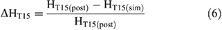
where Hpost is the hazard estimate calculated using the post-fire severity data, and Hsim represents the hazard estimate using the simulated data. In order to calculate differences in hazard estimates for rainfall intensity-duration thresholds, we standardised the difference in 15-min threshold intensity by calculating the proportional difference in estimated threshold between the post-fire and simulated estimate using the equation:
We calculated the difference in hazard estimates for likelihood (ΔHL), volume (ΔHV) and 15-min threshold intensity (ΔHT15) for the eight test burn areas. In addition to the analysis of the distributions of ΔHL, ΔHV and ΔHT15, we also present a case study comparing the predictions based on post-fire and simulated fire severity data with the occurrence of post-fire debris flows in the Las Lomas study basin in the San Gabriel Complex of southern California during the winter of 2016–17.
Results
Histograms representing the distributions of ΔHL, ΔHV and ΔHT15 (by proportion of total segment length) for all eight analysed burn areas are displayed in Fig. 5. The dark grey shaded area in the centre of each of the graphs represents close agreement between simulated and observed estimate values, which we define as a difference of less than 20% for ΔHL (Fig. 5a) and ΔHT15 (Fig. 5b), and within 1000 m3 for ΔHV (Fig. 5c). Frequency data plotted to the left of the shaded area represent the percentage length of modelled stream segment where the simulated estimates were greater than the observed estimates. Frequency data plotted to the right of the shaded area represent the proportional length of modelled stream segment where the simulated estimate was less than the observed estimates.

|
For ΔHL (Fig. 5a) and ΔHV (Fig. 5b), simulated estimates that are lower than observed estimates represented outcomes where the post-fire conditions were estimated to be more hazardous than the simulated conditions (e.g. simulated estimates of likelihood and volume were lower than the observed estimates of likelihood and volume). For ΔHT15 Fig. 5c), simulated estimates that were greater than observed estimates represent outcomes where the post-fire conditions were estimated to be less hazardous than the simulated conditions (e.g. estimated rainfall thresholds based on simulated data are lower than the estimated thresholds based on post-fire data). The proposed method was considered to produce a reasonable approximation of potential debris-flow hazards from the simulated data if a majority of the total stream length had a value of ΔH approaching zero (i.e. most of the proportional length is within the centre grey shaded area). The supplementary material contains maps depicting the results of the modelling for both observed and simulated HL (Fig. S2), HV (Fig. S3) and HT15 (Fig. S4).
Comparison of simulated with post-fire hazard estimates
The results of the estimates of debris-flow hazard derived from simulated fire severity compared favourably with the model predictions based on the post-fire severity data. For debris-flow likelihood, we predicted a majority (>50%) of the total modelled stream segment length to within ΔHL = ±0.2 for all analysed fires in the test dataset (Fig. 5a). Highest accuracies were obtained for the areas burned by the Blue Cut fire and San Gabriel Complex in southern California, whereas least accurate predictions were obtained for the areas burned by the First Creek fire (central WA) and the Pony fire (northern CA).
Debris-flow volume estimates compared favourably between simulated and post-fire data, with >50% of modelled stream segment length within ±1000 m3 ΔHV for six of the eight burn areas (Fig. 5b). The Gap and Pony fires in northern California had the least accurate predictions, with less than 50% of the modelled stream length with ΔHV = ±1000 m3. In the area burned by the Pony fire, estimates of potential volume derived from simulated severity data were greater than those derived from post-fire severity data, whereas post-fire volume predictions were greater than those based on simulated data in the area burned by the Gap fire.
The estimated 15-min rainfall intensity-duration threshold was found to have the lowest predictive accuracy of the three hazard estimates. We determined ΔHT15 was within ±0.2 for >50% of the modelled stream channel length for four of the eight analysed burn areas. The highest levels of predictive accuracy were identified for the area burned by the Blue Cut fire and San Gabriel complex. The least accurate predictions were identified within the areas burned by the First Creek, Gap and Pony fires.
Case study: San Gabriel Complex, winter 2016–17
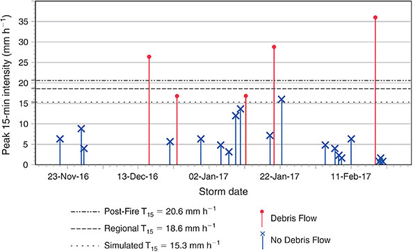
In this section, we present a site-specific analysis of the accuracy of the proposed method as compared with field data collected in the area burned by the San Gabriel Complex. Specifically, we compared predictions of debris-flow hazard based on both simulated and post-fire severity data with debris-flow occurrence (and non-occurrence) information, measurements of debris-flow volume and rainfall intensity-duration data for 29 storm events during the winter of 2016–17 at a monitoring site in the Las Lomas watershed. Individual storms are defined as being separated by a minimum period of 8 h without rainfall, as described by Staley et al. (2013). Storm summary data and modelled hazard estimates for the seven most intense rainfall events can be found in Table 3.

|
Likelihood and rainfall threshold estimates calculated using the observed post-fire severity data correctly predicted debris-flow occurrence for 28 of the 29 rainstorms, while failing to predict the occurrence of a small, short-lived debris flow surge during the storm on 11 January 2017 (Fig. 6 and Table 3). Here, the likelihood model based on post-fire data estimated HL = 0.22 at the measured rainfall intensity of 13.6 mm h−1, which was well below the estimated HT15 of 20.6 mm h−1. The remaining four debris-flow events were associated with rainfall rates that corresponded with HL >0.5 (i.e. a greater than 50% likelihood of debris-flow occurrence).
|
Estimates derived from simulated fire severity correctly predicted debris-flow occurrence for 27 of the 29 storm events that impacted the monitoring watershed (Fig. 6). Simulated data predicted the occurrence of debris flows during storms on 12 January and 21–24 January 2017; however, no debris flows were recorded during this time period. For these storms, the models based on simulated data predicted HL = 0.59 (12 January 2017) and HL = 0.54 (21–24 January 2017) and HT15 = 15.3 mm h−1.
Measurable debris-flow volumes were recorded after three events: 16 December 2016, 20 January 2017 and 18 February 2017 (Table 3). Estimates based on both observed and simulated fire severity data were in close agreement, particularly for the two January debris-flow events. Although both models overpredicted volume by ~100% for the 16 December storm, these estimates were still well within the confidence limits of the volume model where the residual standard error of the estimate (S) = 1.04 (Gartner et al. 2014) is equivalent to a potential volume range of 200–12 000 m3 for using observed fire severity data, and 200–14 000 m3 for simulated fire severity data. Volumetric predictions for the remaining two debris-flow events were much closer to measured values, with post-fire and simulated estimates within 800 and 500 m3 of measured volumes on 20 January 2017, and within 200 and 500 m3 of measured volumes on 18 February 2017.
Discussion
When modelled at a similar historical frequency, we accepted our original hypothesis that estimates based on simulated fire severity data were comparable with those that were calculated using the post-fire burn severity information (Fig. 5). The method also provides hazard estimates that are comparable with field measurements of debris-flow occurrence and magnitude at a monitoring site. We interpreted the degree of predictive accuracy of the simulated estimates as being sensitive to two factors. First, the spatial uniformity of burn severity produced by the wildfire directly affected the predictions of post-fire debris-flow hazard. Here, the highest degree of predictive accuracy was obtained for the southern California burn areas, both of which were characterised by a spatially uniform fire severity, where the San Gabriel Complex was burned mostly at high severity, and the Blue Cut fire burned at mostly moderate severity. The areas burned by the Pony and First Creek fires had a much more spatially variable pattern of fire severity, which resulted in lower predictive accuracies. Second, historical fire occurrence (i.e. a re-burn of the same area) likely affected both dNBR and soil burn severity during subsequent fires. For example, the Pony fire, which was identified as producing a lower degree of predictive accuracy relative to the seven other analysed burn areas, was a re-burn terrain that had been affected by the 2001 Happy Camp Complex and the 2008 Siskiyou–Blue 2 Complex. In this case, dNBR values obtained during post-fire analysis corresponded to a lower soil burn severity than typical for burn areas in this region.
In addition to difficulties in simulating natural spatial patterns of fire severity, implementation of the proposed method for pre-fire prediction requires a priori knowledge or estimation of fire severity. As the historical frequency of a fire cannot be estimated before the occurrence of fire, we recommend the use of a scenario-based approach for the prediction of post-fire debris-flow hazards before wildfire. Specifically, we recommend that fire severity be simulated at three levels of historical frequency: Pdsim = 0.5, 0.75 and 0.9. Here, the dNBR values at the 50th percentile in the CDF (Pdsim = 0.5) represent a moderately frequent fire severity for that vegetation type. The 75th percentile (Pdsim = 0.75) would represent a moderately infrequent degree of fire severity, and the 90th percentile (Pdsim = 0.9) would represent an infrequent, high-severity wildfire.
Here, we provide an example of a scenario-based approach for estimating debris-flow hazards before wildfire for a portion of the Wasatch Front above suburban Salt Lake City, UT, that has not been affected by wildfire in recent decades. Specifically, we focused on three canyons: Ferguson Canyon (3.1 km2), North Fork Deaf Smith Canyon (7.0 km2) and Deaf Smith Canyon (2.2 km2).
An analysis of potential debris-flow hazards revealed a potential for a high degree of hazard at all three scenarios using a design storm with rainfall rates of 24 mm h−1 (results for other storm scenarios with peak 15-min intensities of 12 and 36 mm h−1 can be found in the supplementary material, Figs S5 and S6). Likelihood values were moderate to high in all locations, given steep slopes and high simulated soil burn severities. At Pdsim = 0.5 (Fig. 7a), debris-flow likelihood exceeded 0.6 at the outlet of Ferguson and Deaf Smith Canyons, and was 0.4–0.6 at the outlet of North Fork Deaf Smith Canyon. At Pdsim = 0.75 (Fig. 7d) and Pdsim = 0.9 (Fig. 7g), debris-flow likelihood exceeded 0.6 for all canyon outlets, with likelihood values exceeding 0.8 at the highest simulated fire severity.

|
Despite increases in debris-flow likelihood with increasing fire severity, estimated volumes were similar for the three scenarios, owing to little change in the total amount of simulated area estimated to burn at high or moderate severity. For all scenarios, volumes were estimated to be between 10 000 and 100 000 m3 for the outlets of Ferguson and Deaf Smith Canyon, and >100 000 m3 for the outlet of North Fork Deaf Smith Canyon (Fig. 7b, e and h).
Our model estimated modest 15-min rainfall intensity-duration at all three canyon outlets (Fig. 7c, f and j). Here, we report the 15-min rainfall intensities that equate to a likelihood = 0.5 as the rainfall intensity-duration threshold, after Staley et al. (2017). For each scenario, all three canyon outlets were estimated to have a rainfall intensity-duration threshold of <20 mm h−1, a rate equivalent to a storm with a less than 1-year recurrence interval (NOAA 2016).
Given the high relief and steep terrain within these three canyons, outside of prescribed burning, traditional mitigation strategies that are intended to reduce runoff, stabilise surficial hillslope material, and decrease the volume and velocity of surface runoff may be of limited effectiveness. Instead, risk reduction strategies such as debris-flow early warning, evacuation plans and protective measures that trap sediment (e.g. large sediment retention basins) and constrain channelised flow, should be considered the most effective measures for reducing public exposure to debris-flow hazards.
Conclusions
In the western United States, intense debris-flow generating precipitation associated with convective summer thunderstorms can be concurrent with wildfire, leaving land managers, emergency managers and local officials little time to reduce public exposure to post-fire debris-flow hazards during and after wildfire. As such, accurate estimates of potential debris-flow hazards before wildfire would be beneficial for identifying and prioritising areas in need of risk reduction projects and emergency management strategies, and for implementing mitigation projects to reduce the potential impact of debris flows on communities, infrastructure and important natural and cultural resources. We present a simple, computationally efficient method for estimating potential debris-flow hazards using a statistical approach based on the historical frequency of fire severity, as measured by dNBR and soil burn severity. The proposed method provides estimates of debris-flow hazard based on simulated data that compare favourably with estimates made using fire severity data collected following wildfire.
In addition, the method presented here provides accurate estimates of post-fire debris-flow likelihood and magnitude and rainfall intensity-duration threshold, for a small debris-flow monitoring site in the San Gabriel Mountains of southern California. Despite the accuracy of the method compared with post-fire modelling and field observations, we do not consider the presented method a substitute for a post-fire debris-flow hazard assessment (e.g. Staley et al. 2016, 2017; USGS 2018a). A reanalysis of the area of interest using observed dNBR and field-validated soil burn severity data following wildfire is necessary to better characterise natural patterns of fire severity that are not considered in the present pre-fire analysis.
This method can easily be applied to unburned areas using a scenario-based approach for simulating fire severity, as illustrated by our example of the Wasatch Front above suburban Salt Lake City. The scenario-based approach provides estimates of likelihood, volume and rainfall intensity-duration threshold for a variety of potential fire severities that can be used for pre-fire planning and decision making. As hazard mitigation and risk reduction strategies are often time-consuming to organise and implement, and costly to put in place, pre-fire awareness of the potential debris-flow hazards following wildfire using the proposed method permits better-informed decision support and a longer timeframe for developing future risk mitigation strategies.
The simulation methods presented here may also be directly applicable to other locations, and other areas of wildfire research. Whereas the analysis is specific to the western United States, it would be possible to apply this method to other regions through the analysis of globally available Landsat imagery. However, this approach would require the calculation of a regional vegetation cover database similar to the LandFire project (LandFire 2017). Furthermore, the analysis of the historical distribution of dNBR and soil burn severity within different types of vegetation may be useful for improving our understanding of historical patterns and the temporal changes in fire severity associated with a changing climate. Finally, the methods presented here are directly applicable to modelling other forms of post-fire hazards before wildfire, including flooding and erosion risk, as prediction of both hazards requires input data characterising the severity of wildfire.
Conflicts of interest
The authors declare no conflict of interest.
Acknowledgements
The authors would like to acknowledge the efforts of Robert Leeper (University of California at Riverside) in collecting volumetric data at the Las Lomas study basin. Jonathan Godt and Jeff Coe (USGS) and two anonymous reviewers provided comments and suggestions that improved this manuscript.
References
Cannon SH (2001) Debris-flow generation from recently burned watersheds. Environmental & Engineering Geoscience 7, 321–341.| Debris-flow generation from recently burned watersheds.Crossref | GoogleScholarGoogle Scholar |
Cannon SH, Gartner JE, Wilson R, Bowers J, Laber J (2008) Storm rainfall conditions for floods and debris flows from recently burned areas in south-western Colorado and southern California. Geomorphology 96, 250–269.
| Storm rainfall conditions for floods and debris flows from recently burned areas in south-western Colorado and southern California.Crossref | GoogleScholarGoogle Scholar |
Cannon SH, Gartner JE, Rupert MG, Michael JA, Rea AH, Parrett C (2010) Predicting the probability and volume of post-wildfire debris flows in the intermountain western United States. Geological Society of America Bulletin 122, 127–144.
| Predicting the probability and volume of post-wildfire debris flows in the intermountain western United States.Crossref | GoogleScholarGoogle Scholar |
Eidenshink J, Schwind B, Brewer K, Zhu Z-L, Quayle B, Howard S (2007) A project for monitoring trends in burn severity. The Journal of the Association for Fire Ecology 3, 3–21.
| A project for monitoring trends in burn severity.Crossref | GoogleScholarGoogle Scholar |
Finney MA (2006) An overview of FlamMap fire modeling capabilities. In ‘Fuels management – How to measure success: conference proceedings’, Portland, OR, March 28–30 2006. USDA Forest Service, Proceedings RMRS-P-41, pp. 213–220. (Fort Collins, CO).
Finney MA, McHugh CW, Grenfell IC, Riley KL, Short KC (2011) A simulation of probabilistic wildfire risk components for the continental United States. Stochastic Environmental Research and Risk Assessment 25, 973–1000.
| A simulation of probabilistic wildfire risk components for the continental United States.Crossref | GoogleScholarGoogle Scholar |
French NHF, Kasischke ES, Hall RJ, Murphy KA, Verbyla DL, Hoy EE, Allen JL (2008) Using Landsat data to assess fire and burn severity in the North American boreal forest region: an overview and summary of results. International Journal of Wildland Fire 17, 443–462.
| Using Landsat data to assess fire and burn severity in the North American boreal forest region: an overview and summary of results.Crossref | GoogleScholarGoogle Scholar |
Gartner JE, Cannon SH, Santi PM (2014) Empirical models for predicting volumes of sediment deposited by debris flows and sediment-laden floods in the transverse ranges of southern California. Engineering Geology 176, 45–56.
| Empirical models for predicting volumes of sediment deposited by debris flows and sediment-laden floods in the transverse ranges of southern California.Crossref | GoogleScholarGoogle Scholar |
Haas JR, Thompson M, Tillery A, Scott JH (2016) Capturing spatiotemporal variation in wildfires for improving postwildfire debris-flow hazard assessments. In ‘Natural hazard uncertainty assessment’ (Eds K Riley, P Webley, M Thompson and K Riley.) pp. 301–317. (John Wiley & Sons, Inc.: New York, NY)
Holden ZA, Morgan P, Evans JS (2009) A predictive model of burn severity based on 20-year satellite-inferred burn severity data in a large south-western US wilderness area. Forest Ecology and Management 258, 2399–2406.
| A predictive model of burn severity based on 20-year satellite-inferred burn severity data in a large south-western US wilderness area.Crossref | GoogleScholarGoogle Scholar |
Homer C, Dewitz J, Fry J, Coan M, Hossain N, Larson C, Herold N, McKerrow A, VanDriel JN, Wickham J (2007) Completion of the 2001 National Land Cover Database for the conterminous United States. Photogrammetric Engineering and Remote Sensing 73, 337–341.
Hudak D, Tiryakioğlu M (2009) On estimating percentiles of the Weibull distribution by the linear regression method. Journal of Materials Science 44, 1959
| On estimating percentiles of the Weibull distribution by the linear regression method.Crossref | GoogleScholarGoogle Scholar |
Kean JW, Staley DM, Cannon SH (2011) In situ measurements of post-fire debris flows in southern California: comparisons of the timing and magnitude of 24 debris-flow events with rainfall and soil moisture conditions. Journal of Geophysical Research 116,
| In situ measurements of post-fire debris flows in southern California: comparisons of the timing and magnitude of 24 debris-flow events with rainfall and soil moisture conditions.Crossref | GoogleScholarGoogle Scholar |
Keane RE, Morgan PM, Dillon GK, Sikkink PG, Karau EC (2013) A fire severity mapping system for real-time fire management applications and long-term planning: the FIRESEV project. Available at https://digitalcommons.unl.edu/jfspresearch/18/ [Accessed 25 July 2018].
Keeley JE (2009) Fire intensity, fire severity and burn severity: a brief review and suggested usage. International Journal of Wildland Fire 18, 116–126.
| Fire intensity, fire severity and burn severity: a brief review and suggested usage.Crossref | GoogleScholarGoogle Scholar |
Key CH, Benson NC (2006) Landscape Assessment (LA) sampling and analysis methods. In: FIREMON: Fire effects monitoring and inventory system. Gen. Tech. Rep. RMRS-GTR-164-CD. (Eds DC Lutes, RE Keane, JF Caratti, CH Key, NC Benson, S Sutherland, LJ Gangi) p. LA-1-55. (U.S. Department of Agriculture, Forest Service, Rocky Mountain Research Station: Fort Collins, CO)
Kolden CA, Smith AMS, Abatzoglou JT (2015) Limitations and utilisation of Monitoring Trends in Burn Severity products for assessing wildfire severity in the USA. International Journal of Wildland Fire 24, 1023–1028.
| Limitations and utilisation of Monitoring Trends in Burn Severity products for assessing wildfire severity in the USA.Crossref | GoogleScholarGoogle Scholar |
Lancaster JT, McCrea SE, Short WR (2014) Assessment of post-fire runoff hazards for pre-fire hazard mitigation planning – southern California. Fire Ecology 234, 201
LandFire (2017) Existing vegetation type. Available at https://www.landfire.gov/index.php [Accessed 25 July 2018].
Lutz JA, Key CH, Kolden CA, Kane JT, van Wagtendonk JW (2011) Fire frequency, area burned, and severity: a quantitative approach to defining a normal fire year. Fire Ecology 7, 51–65.
| Fire frequency, area burned, and severity: a quantitative approach to defining a normal fire year.Crossref | GoogleScholarGoogle Scholar |
MTBS (2017) Monitoring Trends in Burn Severity. Available at http://www.mtbs.gov/index.html [Accessed 25 July 2018].
NOAA (2016) Hydrometeorological Designs Study Center Precipitation Frequency Data Server (PFDS). Available at http://hdsc.nws.noaa.gov/hdsc/pfds/index.html [Accessed August 2018].
Parson A, Robichaud PR, Lewis SA, Napper C, Clark JT (2010) Field guide for mapping post-fire soil burn severity. USDA Forest Service, Rocky Mountain Research Station, General Technical Report RMRS-GTR-243. (U.S. Department of Agriculture, Forest Service, Rocky Mountain Research Station: Fort Collins, CO)
Picotte JJ, Peterson B, Meier G, Howard SM (2016) 1984–2010 trends in fire burn severity and area for the conterminous US. International Journal of Wildland Fire 25, 413–420.
| 1984–2010 trends in fire burn severity and area for the conterminous US.Crossref | GoogleScholarGoogle Scholar |
Rollins MG (2009) LANDFIRE: a nationally consistent vegetation, wildland fire, and fuel assessment. International Journal of Wildland Fire 18, 235–249.
| LANDFIRE: a nationally consistent vegetation, wildland fire, and fuel assessment.Crossref | GoogleScholarGoogle Scholar |
Rollins MG, Morgan P, Swetnam T (2002) Landscape-scale controls over 20th century fire occurrence in two large Rocky Mountain (USA) wilderness areas. Landscape Ecology 17, 539–557.
| Landscape-scale controls over 20th century fire occurrence in two large Rocky Mountain (USA) wilderness areas.Crossref | GoogleScholarGoogle Scholar |
Roy DP, Boschetti L, Trigg SN (2006) Remote sensing of fire severity: assessing the performance of the normalized burn ratio. IEEE Geoscience and Remote Sensing Letters 3, 112–116.
| Remote sensing of fire severity: assessing the performance of the normalized burn ratio.Crossref | GoogleScholarGoogle Scholar |
Shakesby R, Doerr S (2006) Wildfire as a hydrological and geomorphological agent. Earth-Science Reviews 74, 269–307.
| Wildfire as a hydrological and geomorphological agent.Crossref | GoogleScholarGoogle Scholar |
Staley DM (2018) Data used to characterize the historical distribution of wildfire severity in the western United States in support of pre-fire assessment of debris-flow hazards: US Geological Survey Data Release. Available at https://www.sciencebase.gov/catalog/item/5b2d0704e4b040769c10b72c [Accessed 25 July 2018].
Staley DM, Kean JW, Cannon SH, Schmidt KM, Laber JL (2013) Objective definition of rainfall intensity–duration thresholds for the initiation of post-fire debris flows in southern California. Landslides 10, 547–562.
| Objective definition of rainfall intensity–duration thresholds for the initiation of post-fire debris flows in southern California.Crossref | GoogleScholarGoogle Scholar |
Staley DM, Negri JA, Kean JW, Laber JL, Tillery AC, Youberg AM (2016) Updated logistic regression equations for the calculation of post-fire debris-flow likelihood in the western United States. US Geological Survey Open-File Report 2016–1106.
Staley DM, Negri JA, Kean JW, Laber JL, Tillery AC, Youberg AM (2017) Prediction of spatially explicit rainfall intensity–duration thresholds for post-fire debris-flow generation in the western United States. Geomorphology 278, 149–162.
| Prediction of spatially explicit rainfall intensity–duration thresholds for post-fire debris-flow generation in the western United States.Crossref | GoogleScholarGoogle Scholar |
Stevens MR, Flynn JL, Stephens VC, Verdin KL (2011) Estimated probabilities, volumes, and inundation depths of potential post-wildfire debris flows from Carbonate, Slate, Raspberry and Milton Creeks, near Marble, Gunnison County, Colorado. US Geological Survey Scientific Investigations Report 2011–5047.
Tillery AC, Haas JR (2016) Potential post-wildfire debris-flow hazards – A pre-wildfire evaluation for the Jemez Mountains, north-central New Mexico. US Geological Survey Scientific Investigations Report 2016–5101.
Tillery AC, Haas JR, Miller LW, Scott JH, Thompson MP (2014) Potential post-wildfire debris-flow hazards – a pre-wildfire evaluation for the Sandia and Manzano Mountains of surrounding areas, central New Mexico. US Geological Survey Scientific Investigations Report 2014–5161.
U.S. Forest Service (USFS) (2018) Remote Sensing Application Center Burned Area Emergency Response imagery support. Available at https://fsapps.nwcg.gov/afm/baer/download.php [Accessed 18 June 2018].
U.S. Geological Survey (USGS) (2018a) Emergency assessment of post-fire debris-flow hazards. Available at http://landslides.usgs.gov/hazards/postfire_debrisflow/ [Accessed 25 July 2018].
U.S. Geological Survey (USGS) (2018b) Post-fire debris-flow hazards. Available at https://landslides.usgs.gov/hazards/ [Accessed 25 July 2018].
Wells WG (1987) The effects of fire on the generation of debris flows in southern California. Reviews in Engineering Geology 7, 105–114.
| The effects of fire on the generation of debris flows in southern California.Crossref | GoogleScholarGoogle Scholar |
1 MTBS data for 2015 became available after analysis for the present manuscript had been completed.