Consumer assessment of eating quality – development of protocols for Meat Standards Australia (MSA) testing
R. Watson A E , A. Gee B , R. Polkinghorne C and M. Porter DA Department of Mathematics and Statistics, University of Melbourne, Vic. 3010, Australia.
B Cosign, 20 Eleventh Avenue, Sawtell, NSW 2452, Australia.
C Marrinya Agricultural Enterprises, 70 Vigilantis Road, Wuk Wuk, Vic. 3875, Australia.
D 2 Oliver Street, Ashburton, Vic. 3147, Australia.
E Corresponding author. Email: rayw@ms.unimelb.edu.au
Australian Journal of Experimental Agriculture 48(11) 1360-1367 https://doi.org/10.1071/EA07176
Submitted: 12 June 2007 Accepted: 20 June 2008 Published: 16 October 2008
Abstract
Meat Standards Australia sought a consistent measure of the beef eating experience to the consumer. Rather than objective measurements or trained panel sensory assessment, it was decided to proceed with direct consumer assessment. Consumer-based assessment has much greater variation, but it has the decided advantage of validity. This paper summarises the path taken to obtain consistent consumer assessment. What meat samples to present to consumers? What responses to ask for? What to do with these responses when they were obtained? The answers to these questions have led to the MQ4 measure of consumer assessment of meat eating quality, which now forms the basis of the MSA predictive model.
Introduction
As discussed by Polkinghorne et al. (2008), support for development of the Meat Standards Australia (MSA) beef grading system came from the 1996 Meat Industry Strategic Plan, where three of the six objectives involved the need for better description of product and marketing systems which would deliver a more consistent beef eating experience to the consumer. Early planning identified the need for a technique by which beef eating quality could be routinely measured. If effective, this methodology could be applied to systematically benchmark the existing retail product and establish or verify the effects and interactions of all product and processing factors.
Options for measuring meat quality included consumer or trained taste panels and objective measurements. Whilst objective measurements (such as shear force and compression) have the advantage of being relatively cheap, they are rather simplistic, one-dimensional measures of a complex set of interactions which occur when cooked meat is chewed and masticated in the mouth. Perry et al. (2001) examined the relationship between objective and sensory measurements and concluded that, whilst shear force was a useful indicator of sensory tenderness, it did not account for all the improvement in sensory scores when meat was aged. This relates to the decreasing importance of the strength of the myofibrillar component of toughness with aging. Further, it was difficult to predict the sensory juiciness scores from objective measurements of meat texture or cooking loss.
Huffman et al. (1996) reported that consumer ratings were consistent with Warner–Bratzler shear values. While they state that this shows consumers can accurately evaluate tenderness, for MSA purposes the salient question was could Warner–Bratzler values predict consumer satisfaction? Further concerns regarding the level of correlation between Warner–Bratzler shear and sensory responses are reported by Poste et al. (1993).
Sensory assessment of meat can be undertaken using either a trained panel of experts or an untrained consumer panel. If we obtain a representative sample of m consumers (who like red meat cooked to medium doneness and are aged between 20 and 50 years), then this will give an unbiased estimate of the population mean of m consumers’ scores for any particular piece of meat.
Trained taste panels are trained to score the specific attributes of eating quality, independently of the other sensory dimensions. A trained panel of tasters yields a smaller spread of scores. This is, after all, part of the purpose of the training. The training to produce consistency generates a modification in the scoring: it reduces the variance of the scores; it may also alter the mean score.
The statistical issue is a balance between validity and reliability; objective measures and trained panels generally produce a more reliable result (smaller variance), but the result may not be valid (incorrect mean). If the sample of consumers is correctly obtained, the consumer results are valid (correct mean) but may not be as reliable (larger variance).
The MSA decision to use consumer taste panels was influenced by the need to have a reliable, transparent system of testing samples that would engender confidence with both the beef industry and consumer sectors. It would also allow the final assessment of palatability to be determined by the target consumer market for the product. To be effective, a robust protocol for testing was required. As the quantity of samples to be tested was unknown, as were the number and nature of factors to be tested, the testing process needed to be sufficiently robust to be effective across any number of experiments over a continuous timeframe. As the trial designs would necessarily change for various experiments, with formal experiments also being interspersed with industry trials and random product testing, the testing protocols and data handling procedures needed to provide the unifying common link to a master database for analysis.
The decision to use random consumers as the test vehicle dictated a need to develop procedures which could satisfactorily evaluate data expected to be highly variable. The objective was to minimise variation for all elements other than individual consumer assessments and the product being tested. This required rigorous, highly controlled test procedures coupled with an agreed system to produce a consumer judgement for evaluation.
Prior to agreeing a final protocol, a major questionnaire was developed and circulated to interested parties (including both Australian and selected overseas sensory organisations) in February 1997. This addressed all stages from product collection and ticketing through to preparation, cooking, serving, consumer selection and scoring. Data from several previous experiments were also evaluated to address issues relating to presentational order, first position anchors, freezing and characteristics of consumer scoring.
A meeting of scientists with an interest in sensory testing along with potential providers was then held to discuss and resolve the issues raised by the questionnaires. This meeting achieved a consensus view on principles that formed the basis for the protocol. The adopted protocol included elements of existing protocols in use by Australian sensory groups and the American Meat Science Association (AMSA 1995), in addition to further features agreed by consensus. Whilst the original written protocol has since been expanded to include more precise operational detail and additional cooking methods, the basic procedures and operations still align closely with the original.
In this paper, key design and operational features of the protocol are documented, in particular the development of a composite meat quality score to provide the consumer measurement standard. The three experiments reported were conducted before the formal MSA program commenced and were used both in establishing some operational test procedures and in establishing the MSA consumer scoring procedure. This was then validated by analysing results from the first eight consumer taste panels (each comprising 180 consumers) conducted under the established grill protocol. Initial revalidation was via analysis of the first 49 grill taste panels, and the first 51 roast taste panels (each of 60 consumers).
Materials and methods
Cooking procedures
Over a period of years, additional cooking methods have been utilised in MSA research to broaden the prediction model and provide a means of improving consumer satisfaction while better utilising traditional secondary cuts. The initial testing was all with grilled steaks. Roasting was then added, with stir fry and slow cooking (casserole) techniques added later. A variety of thin slice cooking techniques, reflecting Asian traditions for wet and dry heat methods, have been adopted most recently.
In each case, detailed protocols have been documented (Gee et al. 2005) to provide for consistency across time and venues. The principal objective has been to reflect a normal consumer product and to remove sources of potential variation in the preparation, cooking and serving process. This is of particular importance due to the nature of the program in which data is pooled over time to enable analysis from a master database in addition to analysing individual experiments. A summary of the procedures adopted for each cooking method can be found in the Accessory Publication in the online version of this paper.
Experiment 1
In this experiment, 80 consumers evaluated 120 striploin samples in a 2 × 2 factorial design, with factors chilling (two chilling rates) and electrical stimulation (yes/no). Product was prepared fresh and tested at 14 days aging. This produced six test product categories. A seventh anchor product of either presumed high or low quality was also tested. Four consumers evaluated each sample (two steaks which were halved after cooking), with consumers grouped as pairs, served halves of a common steak and testing seven samples in all. While the two consumers in each pair were constant with each other, they were combined with a different seven pairs across samples. Samples from each of the products were rotated for presentational order. Steaks were grilled on a Silex clamshell grill to medium doneness following procedures later adopted in the protocols. Consumers preferring a medium degree of doneness were selected by screening and completed a score sheet which included anchored line scales for 13 attributes (dryness, ease of first bite, tenderness, liking of taste, liking of texture, liking of cooked appearance, overall liking, typical beef flavour, flavour, fatty taste, juiciness, hardness and ease of chew).
Experiment 2
This experiment utilised a different group of 60 consumers to evaluate several potential testing issues. Other consumers were again screened for preferring medium doneness, with preparation and cooking procedures also constant. In this trial a common first position link product was served to all consumers before six test samples. A 6 × 6 Latin square design was instituted to present each product an equal number of times in each presentational order position and equally before and after each other product. Only five carcasses were used. The first position link product, prepared from two striploins (M. longissimus dorsi lumborum), was served to 32 and 28 consumers. Samples of steaks of five striploins from the test carcasses were served to each of 24 consumers, with samples from the rump (M. gluteus medius), tenderloin (M. psoas major) and cube roll (M. longissimus dorsi lumorum) served to 16. The scoring scales were reduced to 4, as explained in the Results section below; tenderness, flavour, juiciness and overall satisfaction, and a choice of four categories (unsatisfactory, good everyday, better than everyday and premium quality) were added.
Experiment 3
In this experiment, frozen to fresh product preparation were compared. A total of 72 consumers each evaluated seven products prepared from striploin (M. longissimus dorsi lumborum), rump (M. gluteus medius) and tenderloin (M. psoas major). Cooking procedures were common to the earlier experiments and the four trait questionnaire was again used. Of the 18 cattle utilised, eight were purebred Santa Gertrudis and 10 by Santa Gertrudis sires from Brahman cross Shorthorn females. Each breed group was equally divided into two groups, paired for weight, with nine carcasses receiving electrical stimulation and nine not stimulated.
Striploins (M. longissimus dorsi lumborum) were collected from all carcasses, with an additional four for use as first position links. Rumps (M. gluteus medius) and tenderloins (M. psoas major) were collected from three stimulated carcasses. Two sets of sample steaks were prepared from the 18 striploins, with one set frozen overnight at 14 days aging then thawed for testing the next afternoon to provide a frozen v. fresh comparison. Steaks from the rumps and tenderloins were not frozen.
All consumers received a sample from the four link striploins in first position, 18 consumers testing each. Positions 2 and 3 were alternated between paired frozen and fresh striploin steaks from a common carcass. Half of the consumer groups then tested a rump in position 4, with the other half served a tenderloin. Positions 5 and 6 were a repeat of the frozen v. fresh striploin comparison used in 2 and 3, whereas position 7 was an invert of the rump/tenderloin served in position 4. The design provided for the striploin from each carcass to be served in four positions, twice frozen and twice fresh, to a total of eight consumers. The tenderloins (each served to 18 consumers) and rumps (served to 14 or 18) were presented in two positions producing data suitable for investigating position and carryover effects.
Data from experiments 1, 2 and 3 were evaluated in developing the MSA testing protocols and further to create the MQ4 scoring procedure. All subsequent MSA consumer evaluation has been conducted utilising the developed protocols, with data consolidated into a master database. The early data collected represented a mix of defined specific purpose experiments and a range of cuts collected under controlled conditions, from commercial groups to benchmark beef quality as sold. Results from the first 49 taste panels testing grilled steaks, each comprising 180 consumers testing seven samples, were analysed for each panel to validate the MQ4 scoring procedure. This represented a total of 8820 consumers and 61 740 samples evaluated for the four sensory scales and selected category with four scaled scores. This procedure was repeated for the 60-person roast taste panels, a total of 51 (3060 consumers) being considered. A similar process (data not shown) was followed at later dates as additional cooking methods were added to the program.
Results and discussion
Sensory design issues
The decision to serve seven samples to each consumer was made by consensus following a review of responses to the circulated questionnaire and from analysis of experiments 2 and 3. In experiment 2, where products were rotated for position, the consumer scores were significantly less for positions 6 and 7, indicating the possibility of an order effect, possibly due to tiring. In experiment 3 there were score differences for positions 1, 4 and 7, but these were confounded by the designed use of different cuts in these three positions. An analysis of the remaining four positions, filled by matched fresh and frozen samples, did not find an effect.
Experiment 1 rotated seven test products around the seven presentational positions, whereas experiments 2 and 3 utilised a common first position link product. It was feared that serving, even randomly, a very high or low quality product in first position could bias the relativity of subsequent samples. The correlations in experiments 2 and 3 were larger than in experiment 1, possibly due to the use of a first position anchor or possibly due to more clarity from the reduction in scored attributes. Durier et al. (1997) stated that using a pre-period warm-up product can be useful to ensure better homogeneity between the first period of observation and the next ones. They also observed that, in a pre-period design, a carry over effect was exerted on each product tested removing the need to adjust. While not definitive from the experiments, it was regarded as prudent to incorporate a presumed mid quality link product in the first position. It was also agreed that this product would be served to a large number of consumer pairs to provide a statistical base to compare consumer scores for a common sample in a common position if desired and that, while link scores would be recorded in the database, they would be identified to allow exclusion from general analysis.
Carry-over effects in which a sample’s score is influenced by that tested previously are reported in the literature. Several papers, including those by Durier et al. (1997) and Kunert (1998), discuss design principles to balance these, or to reduce the problem where balance is not possible. Design principles in which all products are tested an equal number of times and appear equally in each position are also reported by these and other authors, with Deppe et al. (2001) describing strategies to counteract situations where complete balance for concurrence, precedence and serving position cannot be attained. Analysis of both experiments 2 and 3 confirmed evident effects with position.
Position and carryover effects were completely balanced in experiment 2 by using a 6 × 6 Latin square design to allocate products to consumers. As this provided balance for order, position and precedence within a link followed by six products arrangement, it was elected to standardise this feature in the protocol. This also reflected the desire for a constant rigorous consumer testing regime that could be automated and used to test a wide range of disparate experimental situations with results being accumulated in a single database.
While a system to grade beef on the basis of predicted consumer satisfaction must necessarily be built on extensive data, it is still desirable to obtain an accurate as possible result on an individual tested cut. In part, this reflects an industry interest in how ‘my animal’ performed but is also useful in grouping cuts for several alternative analyses. For example, cuts from a trial testing electrical stimulation may well be grouped with those from other experiments to investigate marbling or ossification effects. Cuts formerly grouped as a common treatment may then be ungrouped due to differences in marbling and ossification. To reduce position, or session, effects procedures were adopted to allocate portions of any sample tested to five different positions and to serve each within five discrete blocks of consumers within a taste panel. The presentational solutions adopted are further discussed in the Accessory Publication.
In each of the experiments reported, fresh beef samples were presented in an effort to test the normal condition of beef in the retail market. This arrangement, however, was operationally difficult and weakened the ability to relate product results between taste panels as no product could be carried over. This was of particular concern with aging studies where any taste panel differences would confound results. If these problems were to be resolved, freezing of samples was necessary, leading to a further concern that results might be affected by the freezing process. Experiment 3 was devised to test the effect and established that there was no difference between frozen and thawed v. fresh samples. Eight consumers tested paired samples from 18 striploins (M. longissimus dorsi). The results showed no significant difference (t = 0.19, P = 0.85). Accordingly, the protocol established a procedure for all samples to be frozen at the designated aging date and thawed before testing.
A more detailed description of procedures is contained in the Accessory Publication.
Consumer issues
A decision had to be made concerning m, the number of consumers testing one cut. Experiment 2 was structured to include cuts tested by a large number of consumers. Striploin in the link position (M. longissimus dorsi lumborum) was served to 32 and 28 consumers. The five striploins from the test carcasses were each served to 24 consumers, with samples from the rump (M. gluteus medius), tenderloin (M. psoas major) and cube roll (M. longissimus dorsi lumorum) served to 16. Experiment 3 also included large consumer numbers for three cuts; striploin (M. longissimus dorsi lumborum) served to 18 consumers in the link position, rump (M. gluteus medius) served to 14 or 18, and tenderloin (M. psoas major) evaluated by 18.
These data were used to test the balance between test accuracy and the number of consumers per cut and also to test for variation between cuts. More accurate results are obtained by having more observations, but there are two restrictions on this number: (i) physical restrictions – all the meat tested from one cut is supposed to be identical, so we must be able to take m ‘identical’ samples from one cut, and this must be possible for any of the cuts to be tested and even for young animals; and (ii) cost restrictions – the cost increases approximately linearly with m, the standard error decreases only at the rate of √m. This requires a trade-off. What is required is an m that provides sufficient accuracy without excessive cost, variability and outliers. Consumer data have inherent variability and a proportion of outliers, which had to be taken into account, so that m could not be too small. The final decision was to use m = 10.
Scoring systems
In the early sensory work undertaken, a score sheet with thirteen line scales was used. The scales used were:
(1) overall liking (ov)
(2) liking of (cooked) appearance (ap)
(3) liking of texture (tx)
(4) tenderness (tn)
(5) ease of first bite (eb)
(6) ease of chew (ec)
(7) hardness (nhd)
(8) juiciness (ju)
(9) dryness (ndr)
(10) fatty taste (nft)
(11) flavour (fl)
(12) typical beef flavour (bf)
(13) liking of taste (ta).
The ‘n’ is used to denote a reversal of the scale, thus ‘nhd’ denotes the reversed scale from hardness. This is done so that all the variables are positive; a larger value indicates perceived better quality meat. Experiment 1 used this recording format.
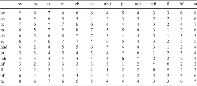
The variable descriptions suggested that there were four or five predominant variables: (i) liking of texture, tenderness, ease of first bite and ease of chew all related to tenderness; (ii) hardness, juiciness, dryness all related to juiciness; (iii) fatty taste, flavour, typical beef flavour, liking of taste all seemed to relate to flavour; and (iv) overall liking, liking of cooked appearance were general variables. The correlation table, Table 1, confirms this trend. It does appear, however, that ta (liking of taste) may fit better with the general variables, rather than with those related to flavour.
|
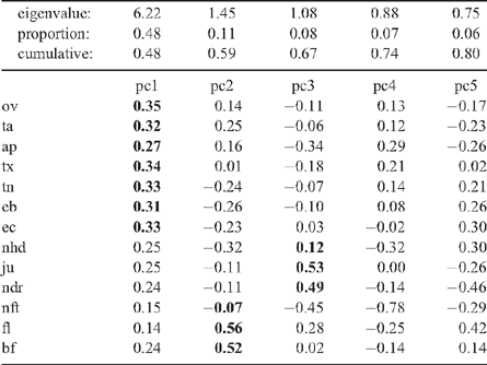
These results suggested reasonable internal consistency. Each consumer tended to rate similarly on all scales; if a product rated highly on one scale then it tended to rate high on the other scales. The most extreme conclusion from this would be that picking any four (for example) of the scales would produce a reasonable product score. However, an improved result could be expected with four that were less correlated with each other (suggesting that they really measure different characteristics). The preliminary analysis suggested that it would be best to choose one variable from each of the four groups. This was further confirmed by a principal components analysis (in which liking of taste was placed with the general variables, see Table 2).
|
Of the first three principal components (those with eigenvalue greater than 1), the first component loads predominantly on the general and tenderness scale, but is not far from an overall average. A surrogate for this might be tenderness and overall liking. The second component loads on the flavour variables, so this could be represented by flavour. The third component loads predominantly on the juiciness variables; this could be represented by juiciness.
On this basis, a weighted average of tn, ov, fl and ju seemed appropriate. The principal components also suggested that most weight should be given to tenderness and overall liking, and least to juiciness.
Thus, it was recommended that the consumer scales be reduced to four: (1) tenderness (tn); (2) juiciness (ju); (3) flavour (fl); and (4) overall liking (ov).
A standard consumer score sheet, reduced to include only these four line scales and the four category boxes, was developed. This was used in experiments 2 and 3.
Following the question ‘Overall how do you rate this sample?’, the response boxes provided a choice of ‘unsatisfactory’, ‘good everyday’, ‘better than everyday’ or ‘premium quality’. These descriptions form the basis for the MSA grade categories: unsatisfactory (X), 3-star, 4-star and 5-star. The consumer questionnaire and a score sheet are presented in the Accessory Publication.
Development of the composite meat quality score: MQ4
Whilst the above analysis indicated that variation in sensory perception could be adequately described by four variables, the problem arose as to how to combine these scores into a single score that could be used as a basis for describing eating quality at an industry level.
A function of tenderness, juiciness, flavour and overall satisfaction which, for a given consumer, best specified ‘meat quality’ as described by the star-rating was sought. A linear discriminant analysis with star as the category to be predicted by tenderness, juiciness, flavour and overall liking was used. For a given set of data, such as a single taste panel, this gave linear functions which specified cut-offs between the star categories of the following form:

Thus, if 0.33 tn + 0.03 ju + 0.10 fl + 0.54 ov < 41.8, the sample is assigned to category X; if 0.33 tn + 0.03 ju + 0.10 fl + 0.54 ov > 41.8, 3-star category; and so on. The result was different from taste panel to taste panel, but the general form was similar: tenderness and overall liking had greater weights, while flavour and juiciness had smaller weights, and often mainly in the higher categories.
As indicated in the example above, the coefficients varied between star categories, but not wildly. In the name of simplicity and transparency, a common discriminant function was adopted, using the same coefficients at each boundary, producing (as an example):

with the star category assigned by determining where MQ4* rated in relation to cut-offs (42.3, 64.7, 79.0; which would be similar to those for the discriminant function): if MQ4* < 42.3, category X; if 42.3 < MQ4* < 64.7, 3-star category; and so on. This performed nearly as well as the discriminant function for data from both experiments 2 and 3, and had the merit of simplicity and specifying one variable.
A 3-scale approach, more in keeping with trained panel sensory practice was also tested using data from experiments 2 and 3. Adopting this approach led to (again, using an example)

This performed nearly as well as the three-variable discriminant function, but quite a bit worse than the four-variable prediction for the same data shown below. Omitting overall liking reduced the accuracy of the prediction. Taking the average of MQ4* and MQ3* produces

This performed very nearly as well as MQ4*. In practice, retention of the overall score added some stability, possibly by smoothing out any erratic movement in the other scores, and resulted in an improvement in discriminatory efficiency. Perhaps, overall may also provide a defacto means of varying the importance of the three base scales across the grades.
These MQ-functions varied with the dataset and the performance changed little with changes in the coefficients, leading to the final recommendation to calculate an MQ4 score by weighting each of the four scale results for each consumer as follows:

The weightings are a compromise between the three- and four-scale approaches, including overall as a component but reducing its importance relative to the statistical best fit values calculated in the four scale studies. This adds some importance to tenderness, which is more critical in defining the difference between unsatisfactory and 3-star product, and also slightly increases the impact of the juicy and flavour components.
This provided a straightforward, easy to apply system, readily explainable to industry, while still achieving acceptable accuracy across all quality levels.
The adopted MQ4 approach was validated by testing MQ4 over a large number of trials (the first 49 grill trials each using 180 consumers and the first 51 roast trials each of 60 consumers) compared with the optimum (the four-variable discriminant function). A typical set of results, giving the proportion of correct classifications, is as follows:
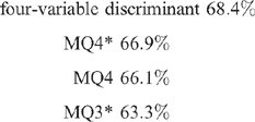
Thus, MQ4 loses little in accuracy, and gains substantially in its simplicity. As can be seen, the four-variable options are better than the three-scale alternatives, with the recommended MQ4 approach close to the optimal, but impractical, position, where grade standards would be reset for any particular taste panel.
The strength of this consumer consensus regarding eating quality provides a powerful argument for grading. If grades are accurately delivered, consumers will agree with the label providing a highly effective basis for marketing.
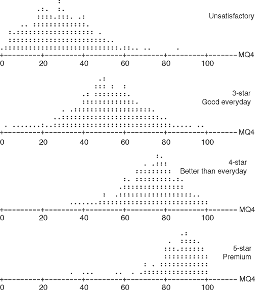
The dot plots shown in Fig. 1 indicate the spread of MQ4 scores v. star category selected for a typical consumer group.
|
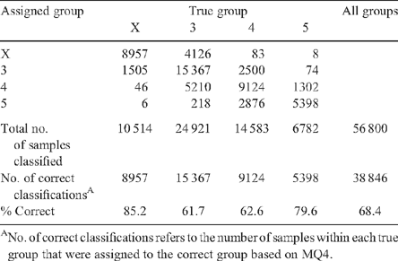
The pattern and spread of consumer MQ4 scores are further illustrated in Table 3, which corresponds to the dot plots given above. The assigned group is obtained by inserting vertical lines around 42, 64 and 80. Those to the left of 42 are assigned to group X, 42−64 to group 3, and so on.
|
As can be seen with the maximum score for an unsatisfactory sample of 86 with one consumer and a minimum 5-star score of 34 for another, it is not possible to achieve a perfect categorisation. Equally evident from the dot plots however is the solid pattern across the population with each grade grouped in a relatively distinct position even allowing for the overlap.
Also obvious is the effect on classification accuracy v. consumer risk in moving a grade boundary. This is well demonstrated at the X/3-star boundary, where a cut-off score of ~42 would deliver the lowest misclassification rate but result in a reasonable quantity of unsatisfactory product receiving a 3-star label. A higher cut-off score of 48 would better protect the consumer from unsatisfactory product, but would also reject a higher percentage of product which was actually of 3-star quality.
An initial fail/3-star boundary of 48 was adopted for MSA grades which were originally based on population pathways. These were supplanted by prediction models which estimated an MQ4 score for each cut from an individual carcass. As the accuracy of the prediction model improved, the failure cut-off score was relaxed to 46.5.
A further issue considered was how to treat consumer scores which were evidently aberrant. Clearly, some consumer scores are ‘wrong’ and consumers have apparently marked the wrong end of the scale or, in a few cases, have not been capable or interested in scoring variations in eating quality. Such observations can seriously bias the result.
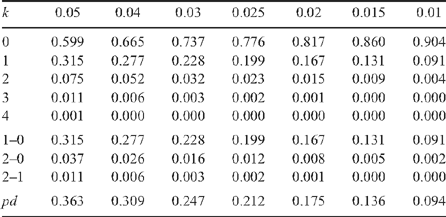
Table 4 gives the probabilities of k = 0, 1, 2, outliers (including missing data) in a random sample of m = 10, when the proportion of outliers among all data is π = 0.05,., 0.01.
|
Initial datasets suggested that the outlier rate was of the order of 5%, but more recent data suggests that the outlier rate is around 2%. Of a sample of 5786 × 10 consumer evaluations, 2.5% differed from the sample median by more than 45, 1.5% by more than 50.
If an outlier is defined, for the present discussion, as an observation deviating by more than 45 from the median, then 2.5% of the data are outliers. If there is one outlier among a group of m = 10, which occurs for ~20% of such groups, then this moves the mean towards the outlier by ~5 points. If there are two outliers (2% of such groups), then in roughly half the cases there is little effect as one is on either side; but in the other half, the effect is twice as bad, moving the mean towards the outlier by ~10 points.
Further, if the median is high (the meat is good), then outliers can only be low as there is no room at the top. Similarly if the median is low, then outliers can only be high. One effect of outliers, therefore, is to bias the means towards the middle of the scale.
So, as explained above, there are two problems created by outliers: (i) possible bias of the estimate; and (ii) an increase in the standard deviation and, therefore, a reduction in the precision of the sample mean as an estimator.
One way to overcome the problem of outliers is to use a trimmed-mean. For a set of m observations x1, x2,…, x m , the order statistics are denoted by x(1), x(2),…, x( m ), which are such that:

The (m − d)-trimmed mean, i.e. the mean of m observations obtained after deleting the d extreme observations, is then given by:

This is the average of the middle (m − d) observations, excluding the d/2 smallest values and the d/2 largest values.
For product p, consumer c makes the following evaluations:

and from these is obtained MQ4 for product p as assessed by consumer c:

The estimated characteristic for product p, is then obtained as the (10−4)-trimmed mean of these evaluations:

This is the mean of the middle six observations, excluding the two smallest and the two largest values. Thus,

This choice of trimmed mean seems reasonable on the basis of the bias considerations. There are seldom more than two outliers in a group of ten, so if we avoid the problems caused by, at most, two outliers, the bias problem is solved.
In using the (untrimmed) mean as an estimate of the centre of the distribution, there are two problems associated with outliers:
-
bias – the outlier distorts the sample mean;
-
efficiency – the outlier increases the sample standard deviation, so that the precision of the sample mean as an estimator is diminished.
In the above consideration of possible bias, we imagine the outliers are being sampled from a distribution other than the one we wish to tap. However, even if all the observations are legitimate (and therefore part of the distribution we want to investigate), then the key would be the efficiency of the estimator, i.e. its standard error. The estimator with the smaller standard error is more efficient.
The standard error of the (m − d)-trimmed mean is given by.

where f = d/m and sW denotes the Winsorised standard deviation (see Staudte and Sheather 1991).
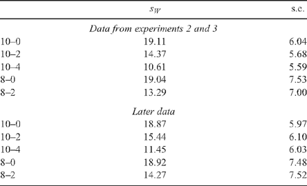
Early data, based on 462 × 10 evaluations from experiments 2 and 3, yielded the results shown in Table 5. These results were supported by simulations based on further data from experiments 2 and 3, for which 24 or 32 observations were available for several cuts.
|
However, subsequent data based on 5786 × 10 evaluations yielded the results presented in Table 5. Presumably reflecting the reduction in the proportion of outliers in the later data, the efficiency of untrimmed sample mean is now marginally better than the trimmed mean, but this assumes that all the outliers are legitimate.
For the initial data, the (10−4)-trimmed mean was clearly superior. With improved consumer data, the trimmed mean was closer; but the proportion of outliers would need to be further reduced before the untrimmed mean was used.
For consumer data, the (10−4)-trimmed mean is still recommended. It provides a robust statistic and, even if all the outliers were legitimate, it would lose little in efficiency.
On the basis of this analysis, a CMQ4 score was adopted which utilised 10 consumers and clipped four:

Possible alternatives to clipping were to use the mean or the median of the 10 scores. The mean is the (10−0)-trimmed mean and the median is the (10−8)-trimmed mean. Thus the (10−4)-trimmed mean is a compromise between the mean and the median. It achieves the advantages of both, while limiting their respective disadvantages.
Conclusions
A consumer testing protocol was generated through a series of trials. Its derivation is explained in the paper and the protocol itself is described in some detail in the Accessory Publication.
The information to be obtained from the consumer was the subject of much study. In terms of the usefulness of consumer responses, asking too much would generate a poor response and asking too little meant an unsatisfactory basis for a measure. It was decided that the number of responses required from a consumer about a particular meat sample be limited to four, in addition to an assessment of the star-rating. The choice of responses was chosen as the best four from an initial set of 13. These responses were combined to produce one measure of meat eating quality.
One obvious problem with consumer data is their reliability. In order to generate a more reliable measure, several consumers were used to judge each piece of meat. Again, there is a trade-off between cost and precision. It was decided that a trimmed mean be used, i.e. a sample of 10 consumers is used, the smallest two and the largest two observations are deleted and the middle six averaged. This gave a robust and reasonably reliable measure, MQ4.
This measure has stood the test of time, and it forms the basis of the MSA consumer prediction model (see Watson et al. 2008). The model predicts MQ4 from available data. This prediction gives a good assessment of the consumer assessment of meat eating quality.
Deppe C,
Carpenter R, Jones B
(2001) Nested incomplete block designs in sensory testing: construction strategies. Food Quality and Preference 12, 281–290.
| Crossref | GoogleScholarGoogle Scholar |
[Verified 14 July 2008]
Huffman KL,
Miller MF,
Hoover LC,
Wu CK,
Brittin HC, Ramsey CB
(1996) Effect of beef tenderness on consumer satisfaction with steaks consumed in the home and restaurant. Journal of Animal Science 74, 91–97.
| PubMed |

Kunert J
(1998) Sensory experiments as crossover studies. Food Quality and Preference 9, 243–253.
| Crossref | GoogleScholarGoogle Scholar |

Perry D,
Thompson JM,
Hwang IH,
Butchers A, Egan AF
(2001) Relationship between objective measurements and taste panel assessment of beef quality. Australian Journal of Experimental Agriculture 41, 981–989.
| Crossref | GoogleScholarGoogle Scholar |

Polkinghorne R,
Thompson JM,
Watson R,
Gee A, Porter M
(2008) Evolution of the Meat Standards Australia (MSA) beef grading system. Australian Journal of Experimental Agriculture 48, 1351–1359.

Poste LM,
Butler G,
Mackie D,
Agar VE, Thompson BK
(1993) Correlations of sensory and instrumental meat tenderness values as affected by sampling techniques. Food Quality and Preference 4, 207–214.
| Crossref | GoogleScholarGoogle Scholar |

Watson R,
Polkinghorne R, Thompson JM
(2008) Development of the Meat Standards Australia (MSA) prediction model for beef palatability. Australian Journal of Experimental Agriculture 48, 1368–1379.


